Scaling of demixing curves and crossover from critical to tricritical behavior in polymer solutions

Abstract

In this paper we show that the virial expansion up to third order for the osmotic pressure of a dilute polymer solution, including first-order perturbative corrections to the virial coefficients, allows for a scaling description of phase-separation data for polymer solutions in reduced variables. This scaling description provides a method to estimate the $\Theta$-temperature, where demixing occurs in the limit of vanishing polymer volume fraction $\phi$ and infinite chain-length $N$, without explicit assumptions concerning the chain-length dependence of the critical parameters $T_{{\rm c}}$ and $\phi_{{\rm c}}$. The scaling incorporates three limiting regimes: the Ising limit asymptotically close to the critical point of phase separation, the pure-solvent limit, and the tricritical limit for the polymer-rich phase asymptotically close to the theta point. We incorporate the effects of critical and tricritical fluctuations on the coexistence curve scaling by using renormalization-group methods. We present a detailed comparison with experimental and simulation data for coexistence-curves and compare our estimates for the $\Theta$-temperatures of several systems with those obtained from different extrapolation schemes.

I Introduction

A quantitative description of the properties of a system in the vicinity of multicritical points remains one of the most interesting problems in the physics of phase transitions. Closeness to a multicritical point leads to a complex crossover between several lines of critical points, which cannot be described in terms of a single universality class. As a rule, the appearance of a multicritical point on the phase transition line is related to the interaction of two or more order parameters [1]. Correspondingly, the complex crossover behavior is affected by a competition between the diverging correlation lengths of the fluctuations of these different order parameters. The most well-known example of such systems with a multicritical (specifically, tricritical) point is the ³He-⁴He mixture [1, 2].

In this paper we investigate the phase separation of solutions of high-molecular-weight polymers in low-molecular-weight solvents in the vicinity of the $\Theta$-point, which is defined as the critical mixing point in the limit of infinite degree of polymerization [3]. De Gennes [4], by mapping Edwards’ continuous chain model onto a Euclidean field theory in the formal limit of zero spin components, has argued that the $\Theta$-point in the polymer-solvent system is a tricritical point. A tricritical point separates lines of second-order ($\lambda$-line) and first-order (triple-line) transitions. The states above the $\Theta$-temperature on the line of zero polymer volume fraction $\phi=0$, shown by the dotted line in Fig. 1, correspond to the critical self-avoiding-walk singularities associated with the behavior of long $(N\rightarrow\infty)$ polymer molecules at infinite dilution [5, 6]. Later on, the mapping onto a field theory was generalized to solutions of finite concentration and arbitrary polydispersity [3, 7, 8, 9, 10]. The scaling field ${\bf{h}_{1}}$, conjugate to the polymer order parameter $\psi\,$, is zero along the $\lambda$-line but becomes non-zero for finite degrees of polymerization $N$. The second scaling field $h_{2}$ (scalar) conjugate to $\psi^{2}$ also vanishes in the limit of infinite $N$ and zero polymer volume fraction. The correlation length associated with the polymer order parameter is proportional to the radius of gyration of a polymer which diverges in the limit of infinite degree of polymerization. Below the (tricritical) $\Theta$-point the polymer order parameter exhibits a discontinuity accompanied by a phase separation and by a discontinuity in the concentration of the polymer. The line of critical phase-separation points shown in Fig. 1 is a nonzero-field critical (“wing”) line originating from the tricritical point. The order parameter for the fluid-fluid phase separation, associated with the volume fraction of monomers $\phi$, and the polymer order parameter $\psi\,$belong to different universality classes. Tricriticality emerges as a result of a competition between these two order parameters and exhibits mean-field behavior with logarithmic corrections [11, 12, 13]. Specifying the precise physical meaning of the polymer order parameter $\psi\,$is a bit complicated (see Ref. [3] p. 287f). In analogy to the $\lambda$-transition in ⁴He, one can view $\psi\,$$({\bf{r})}$ as an operator for initiation or termination of a polymer chain at a point ${\bf{r}}$, thereby relating it to the concentration of polymer endpoints. On the level of two-point correlations, one finds that the transverse correlations of $\psi\,$are related to the correlations of the ends of a single polymer, while the longitudinal correlations (in the direction of ${\bf{h}_{1}}$) are related to the correlations between all chain ends [7, 8, 9]. A full description of the phase separation near the tricritical point should incorporate a crossover between Ising critical behavior on the wing critical line and tricritical behavior close to the $\Theta$-point.

The separation of a polymer solution into two coexisting phases has been qualitatively explained long ago by Flory and Huggins [14]. However, the Flory-Huggins theory describes the phase separation only qualitatively, because it is based on a mean-field lattice model which neglects fluctuations. It leads to the following Helmholtz free energy $F$ of mixing of polymer chains and solvent molecules [3, 15]:

$$\frac{F}{\Omega k_{{\rm B}}T}\equiv f=(1-\phi)\ln(1-\phi)+\frac{\phi}{N}\ln\phi+\frac{\Theta}{2T}\phi(1-\phi),$$ (1)

where $\Omega$ is the number of lattice sites in the system, $k_{{\rm B}}$ Boltzmann’s constant, $T$ the temperature, while $\phi$ is the volume fraction of the polymer, and $\Theta$ is the $\Theta$-temperature. We obtain the Gibbs free energy $G$ via the Legendre transformation $G=F+PV$, where $P$ is the pressure and $V=\Omega l^{3}$, with $l$ being the length of a lattice cell. From the Gibbs free energy one can calculate the chemical potential $\mu_{{\rm P}}$ of the polymer and $\mu_{{\rm S}}$ of the solvent [15]

$$\hat{\mu}_{{\rm P}}(\phi,P,T) \equiv \mu_{{\rm P}}(\phi,P,T)-\mu_{{\rm P}}^{0}(T)=k_{{\rm B}}T\left(f+(1-\phi)\frac{\partial f}{\partial\phi}\right)+Pl^{3}\,,$$ (2)

$$\hat{\mu}_{{\rm S}}(\phi,P,T) \equiv \mu_{{\rm S}}(\phi,P,T)-\mu_{{\rm S}}^{0}(T)=k_{{\rm B}}T\left(f-\phi\frac{\partial f}{\partial\phi}\right)+Pl^{3}\,,$$ (3)

which obey the relation $G/\Omega=\phi\hat{\mu}_{{\rm P}}+(1-\phi)\hat{\mu}_{{\rm S}}$. In Eqs. (2) and (3) $\mu_{{\rm P}}^{0}(T)$ and $\mu_{{\rm S}}^{0}(T)$ are the standard chemical potentials of pure polymer and solvent, respectively. The osmotic pressure $\Pi=-\hat{\mu}_{{\rm S}}/l^{3}+P$, due to the presence of the polymer, is the additional pressure needed to establish equilibrium with the pure solvent across a semipermeable membrane:

$$\hat{\mu}_{{\rm S}}(0,P+\Pi,T)=\hat{\mu}_{{\rm S}}(\phi,P,T)\,.$$ (4)

Using Eq. (3) we find

$$\hat{\Pi}\equiv\frac{\Pi l^{3}}{k_{{\rm B}}T}=\phi\frac{\partial f}{\partial\phi}-f\,.$$ (5)

In the region of phase coexistence for $T<\Theta$, the values $\phi_{1}$ and $\phi_{2}$ of the volume fractions in the coexisting phases are found from the condition of equal chemical potentials (or osmotic pressures) in both phases:

$$\hat{\mu}_{{\rm S}}(\phi_{1},P,T) = \hat{\mu}_{{\rm S}}(\phi_{2},P,T)\,,$$ (6)

$$\hat{\mu}_{{\rm P}}(\phi_{1},P,T) = \hat{\mu}_{{\rm P}}(\phi_{2},P,T)\,,$$ (7)

where the subscript 1 denotes the solvent-rich phase and 2 the polymer-rich phase. Coexistence curves can also be calculated from the free energy by a common-tangent construction

$$\left.\frac{\partial f}{\partial\phi}\right|_{\phi_{1}}=\left.\frac{\partial f}{\partial\phi}\right|_{\phi_{2}}=\frac{f(\phi_{2})-f(\phi_{1})}{\phi_{2}-\phi_{1}}\,,$$ (8)

which determines the two densities $\phi_{1}$ and $\phi_{2}$ of the phase-separated system. At constant pressure and temperature these conditions are equivalent to the equality of the chemical potentials of the polymer and of the solvent in both phases. According to the Flory-Huggins theory [14], the dependence of the critical temperature $T_{{\rm c}}$ and the critical volume fraction $\phi_{{\rm c}}$ of the polymer on the degree of polymerization $N$ is $T_{{\rm c}}=\Theta/(1+1/\sqrt{N})^{2}$ and $\phi_{{\rm c}}=1/(1+\sqrt{N}),$ respectively. As shown by Widom [16], for any value of the variable

$$x=\frac{1}{2}\sqrt{N}(1-T/T_{{\rm c}})\,,$$ (9)

but only if $N$ is large and $T$ is close to $T_{{\rm c}}$, the phase coexistence in the Flory-Huggins theory can be represented by a scaling form: the concentration difference $\phi_{2}-\phi_{1}$, where $\phi_{1}$ and $\phi_{2}$ are the volume fractions of polymer in the concentrated and dilute phases, respectively, is given by

$$\sqrt{N}(\phi_{2}-\phi_{1})\sim\left\{\begin{array}[]{ll}2\sqrt{6x}&(x\rightarrow 0)\\ 3x&(x\rightarrow\infty)\end{array}\right.\,,$$ (10)

where the limit $x\rightarrow 0$ corresponds to the critical point when $T\rightarrow T_{{\rm c}}$ for fixed $N$, and the other limit $x\rightarrow\infty$ is approached when $N\rightarrow\infty$, for fixed $T$.

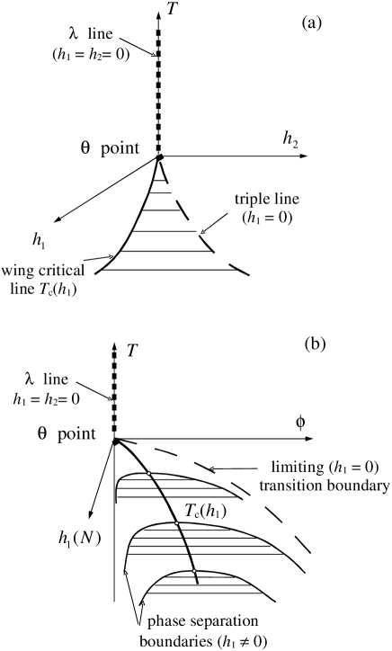
FIG. 1.: Schematic phase diagram near the tricritical $\Theta$-point: (a) shown in field variables $T,h_{1},h_{2}$; at $T=\Theta$ the $\lambda$ line of self-avoiding-walk-type critical behavior ends and a surface of first-order demixing transitions with $h_{1}\neq 0$ emerges, which is bound by the wing line of critical demixing points and by the triple line located at $h_{1}=0$; (b) replacing $h_{2}$ by the density variable $\phi$ reveals two-phase coexistence. Slices at constant chain length $N$, as indicated in the figure, give the familiar phase-coexistence curves.

Asymptotically close to the critical point of phase-separation (the scaling variable $x\rightarrow 0$) the Flory-Huggins theory fails, as does any other mean-field theory which neglects critical fluctuations. The critical behavior of the polymer solution near $T_{{\rm c}}$ is known to belong to the three-dimensional Ising universality class. In particular, in the asymptotic vicinity of the phase-separation critical point the concentration difference $\phi_{2}-\phi_{1}$ as a function of the reduced temperature difference $\tau=(T-T_{{\rm c}})/T_{{\rm c}}$ obeys a power law:

$$\phi_{2}-\phi_{1}\simeq 2B_{0}\left|\tau\right|^{\beta}\,.$$ (11)

However, Ising-like critical behavior is revealed only when the correlation length of the critical density fluctuations is much larger than the radius of gyration of the polymer chain [17, 18]. This fact implies that the Ising region in high-molecular-weight polymer solutions is confined to a very narrow temperature range near the critical point. Outside this region, a crossover to mean-field type behavior is observed. A Flory theory renormalized by critical fluctuations has been developed by Povodyrev et al. [20]. The extent of the Ising region is predicted to narrow with increasing $N$ in a manner governed by the Ginzburg criterion, and disappears entirely in the limit of infinite $N$. For large $N$, the interplay between $\left|\tau\right|$ and $1/\sqrt{N}$ will drive the system from asymptotic Ising critical behavior, when $|\tau|\sqrt{N}\gg 1$, to asymptotic tricritical behavior, $\left|\tau\right|\sqrt{N}\ll 1$, through a region of intermediate crossover behavior.

The approach developed in Ref. [20] contains most essential features of real systems, namely: the crossover from mean-field to asymptotic Ising-like behavior, the crossover to the (tricritical) $\Theta$-behavior, and the variation of the effective critical exponents upon changing the degree of polymerization. However, the restrictions imposed by the free energy (1) of the Flory-Huggins theory are too tight to represent actual data within experimental accuracy. This is why here we shall use a more general approach based on the virial expansion of the osmotic pressure $\Pi$, which we shall renormalize so as to include the effects of fluctuations. We then try to describe existing experimental and simulation data on phase separation in polymer solutions with this approach.

This paper is organized as follows. In Sec. II we briefly review the connection between polymer solutions and field theory and show that the Helmholtz free energy has a scaling form in the mean-field approximation and also if one includes contributions from the first-order perturbation theory. In Sec. III we describe how critical fluctuations renormalize the free energy and in Sec. IV we incorporate the effects of tricritical fluctuations. Sec. V contains a detailed comparison of the renormalized theory with the phase-separation data available from experiments and simulations. In Sec. VI we summarize our findings.

II Mean-field description

Utilitising des Cloizeaux’s mapping between Edwards’ model of polymer solutions in the case of nonzero concentration $\phi$ and a $O(n)$ symmetric field theory in a magnetic field of magnitude $h_{1}$ in the limit $n\rightarrow 0$, we find the following relations between the polymer observables $\phi,\hat{\Pi},c_{{\rm p}}=\phi/N$ and the effective potential $\Gamma(\psi,h_{2})$ of the field theory [3, 7, 8]

$$\phi = \frac{\partial\Gamma}{\partial h_{2}}\,,$$ (12)

$$c_{{\rm p}} = \frac{\psi}{2}\frac{\partial\Gamma}{\partial\psi}\,,$$ (13)

$$\hat{\Pi} = \psi h_{1}-\Gamma\,,$$ (14)

where $c_{{\rm p}}$ is the concentration of polymer molecules, $N$ is the mean degree of polymerization. For the effective potential $\Gamma$, we start from the mean-field expression

$$\Gamma=h_{2}\psi^{2}+\lambda\psi^{4}+v\psi^{6}\,,$$ (15)

which one may interpret as a Landau expansion in terms of $\psi$, but which also emerges as the result of a zero-loop (“tree”) approximation in a field theory or in the Edwards model [12]. We should mention, that des Cloizeaux’s mapping [7] demands a polydisperse grand canonical ensemble with an exponential chain-length distribution, while the experiments that we want to describe are performed with nearly monodisperse samples. A broad chain-length distribution in the experiments would seriously affect the demixing transition, since the chain-length distributions may differ in the phases below the demixing temperature, and thereby may even change the nature of the transition. Polydispersity effects have been incorporated in the theoretical framework for the excluded-volume region, where the effective monomer-monomer interactions are repulsive and therefore $\lambda$ is positive [23, 24]. Fortunately, in the tree approximation the effective potential $\Gamma$ and thereby the osmotic pressure $\hat{\Pi}$ are independent of polydispersity. Also the first-order correction for $\hat{\Pi}$ yields a change of only about $12\%$ when changing from a monodisperse to an exponential chain-length distribution [12]. Therefore, using the mean-field approximation for $\Gamma$, we confidently apply the theory to experiments on nearly monodisperse solutions.

Minimizing Eq. (14) for the osmotic pressure $\hat{\Pi}$ with respect to $\psi$ we find

$$h_{1}=\frac{\partial\Gamma}{\partial\psi}=\psi(2h_{2}+4\lambda\psi^{2}+6v\psi^{4})\,,$$ (16)

for the field $h_{1}$ conjugate to the order parameter $\psi$. Evaluation of (12) and (13) gives

$$\phi = \psi^{2}$$ (17)

$$h_{2} = \frac{1}{N}+2\lambda\psi^{2}+3v\psi^{4}\,.$$ (18)

Using (17) and (18) in Eq. (14) we arrive at the familiar expansion of the osmotic pressure near the $\Theta$-point

$$\hat{\Pi}=\frac{\phi}{N}+\lambda\phi^{2}+2v\phi^{3}\,.$$ (19)

Equation (19) is the virial expansion of the equation of state. Note that integration of Eq. (5) using Eq. (19) for $\hat{\Pi}$ leads to a free energy

$$f=\frac{\phi}{N}\ln\phi+\lambda\phi^{2}+v\phi^{3}\,,$$ (20)

similar to Flory’s expression (1), with the $(1-\phi)\ln(1-\phi)$ term expanded and with the expansion constants replaced by two system-dependent interaction parameters $\lambda$ and $v$. The parameters $\lambda$ and $v$ are expected to be analytic functions of the temperature with $\lambda$ changing its sign at the $\Theta$-temperature, leading to the polymer-chain-collapse transition, while in the tricritical scenario $v$ is positive in order to stabilize the system at a finite density. To lowest order we can write

$$\lambda=\lambda_{0}\frac{T-\Theta}{\Theta}\,,$$ (21)

where $\lambda_{0}>0$ is a system-dependent constant, so that $\lambda$ is negative below the $\Theta$-point and is positive above the $\Theta$-point. The lowest-order approximation for $v$ is simply a constant independent of temperature.

The lambda line is reached for $T>\Theta$ and $h_{1}=h_{2}=0$ (see Fig. 1). At the triple line (coexistence curve in the limit $N\rightarrow\infty$) for $T<\Theta$ we also have $h_{1}=0$ but $h_{2}\neq 0$. At the $\Theta$-point all three fields $h_{1},h_{2}$ and $\lambda$ vanish. In the semi-dilute (sd) limit of polymer concentration $c_{{\rm p}}\rightarrow 0$ at fixed $\phi$ ($i.e.,$ $N\rightarrow\infty$) the osmotic pressure becomes $\hat{\Pi}(\phi)=\phi^{2}(\lambda+2v\phi)$ and one easily finds from the equality of the osmotic pressure in both phases:

$$\phi_{1}=0\qquad\mbox{and}\qquad\phi_{{\rm sd}}=\phi_{2}=-\frac{\lambda}{2v}$$ (22)

for the polymer volume fractions in the coexisting pure solvent phase and semi-dilute phase. Substituting this result in Eq. (16) we note that we approach the symmetry plane $h_{1}=0$ for $N\rightarrow\infty$. In the semi-dilute limit all polymer molecules aggregate in the polymer-rich phase and their overlap $s=R_{{\rm g}}^{3}c_{{\rm p}}$ tends to infinity, because the mean radius of gyration $R_{{\rm g}}$ diverges faster than $c_{{\rm p}}$ vanishes. The critical demixing point can be found from the stability conditions

$$\left(\frac{\partial\hat{\Pi}}{\partial\phi}\right)_{T,N}=\left(\frac{\partial^{2}\hat{\Pi}}{\partial\phi^{2}}\right)_{T,N}=0\,.$$ (23)

Insertion of Eq. (19) yields the critical volume fraction

$$\phi_{{\rm c}}=-\frac{\lambda_{{\rm c}}}{6v}=\frac{1}{\sqrt{6vN}}\,.$$ (24)

¿From Eqs. (22) and (24) we can form the universal ratio $\phi_{{\rm sd}}/\phi_{{\rm c}}=3$, which, since $\lambda\sim T-\Theta$, measures the ratio of the slopes of the wing critical line and the phase separation boundary in the semi-dilute limit. The result $\phi_{{\rm sd}}/\phi_{{\rm c}}=3$ coincides with Flory theory but differs from the result $\phi_{{\rm sd}}/\phi_{{\rm c}}=5/2$ [25, 26] that one finds from the Landau expansion by keeping $h_{2}$ constant instead of $N$ in the calculation of the wing critical line. To our knowledge the only attempt to independently obtain this universal ratio was made in simulations by Frauenkron and Grassberger [27, 28]. Their result $\phi_{{\rm sd}}/\phi_{{\rm c}}\approx 2.9-3.2$ supports the validity of a calculation at constant $N$.

Using the scaled variables

$$\Delta\tilde{\phi} = \frac{\phi-\phi_{{\rm c}}}{\phi_{{\rm c}}}\,,$$ (25)

$$\Delta\tilde{\lambda} = \frac{\lambda-\lambda_{{\rm c}}}{\lambda_{{\rm c}}}\,,$$ (26)

and the mean-field result (24), we find that the osmotic pressure (19) obeys the scaling form

$$\Delta\tilde{\Pi}=\frac{\hat{\Pi}-\hat{\Pi}_{{\rm c}}}{\hat{\Pi}_{{\rm c}}}=-3\Delta\tilde{\lambda}(1+\Delta\tilde{\phi})^{2}+(\Delta\tilde{\phi})^{3}\,,$$ (27)

with $\hat{\Pi}_{{\rm c}}=2v\phi_{{\rm c}}^{3}$ and without explicit system-dependent parameters. To obtain the scaling equation for the free energy we subtract its regular part

$$f_{{\rm reg}}=f(\phi_{{\rm c}})+\left.\frac{\partial f}{\partial\phi}\right|_{\phi_{{\rm c}}}(\phi-\phi_{{\rm c}})\,,$$ (28)

which neither does contribute to the susceptibility nor affects the calculation of coexistence curves. With this subtraction we find

$$\Delta\tilde{f}\equiv\frac{f-f_{{\rm reg}}}{\hat{\Pi}_{{\rm c}}}=3[(1+\Delta\tilde{\phi})\ln(1+\Delta\tilde{\phi})-\Delta\tilde{\phi}-\left(\Delta\tilde{\lambda}+\frac{1}{2}\right)(\Delta\tilde{\phi})^{2}+\frac{1}{6}(\Delta\tilde{\phi})^{3}],$$ (29)

and the coexistence curve is calculated from the conditions

$$\left.\frac{\partial\Delta\tilde{f}}{\partial\Delta\tilde{\phi}}\right|_{\Delta\tilde{\phi}_{1}}=\left.\frac{\partial\Delta\tilde{f}}{\partial\Delta\tilde{\phi}}\right|_{\Delta\tilde{\phi}_{2}}=\frac{\Delta\tilde{f}(\Delta\tilde{\phi}_{2})-\Delta\tilde{f}(\Delta\tilde{\phi}_{1})}{\Delta\tilde{\phi}_{2}-\Delta\tilde{\phi}_{1}}\,.$$ (30)

The Ansatz (21) for the temperature dependence of $\lambda$ gives

$$\Delta\tilde{\lambda}=\frac{T-T_{{\rm c}}}{T_{{\rm c}}-\Theta}\,,$$ (31)

for the scaling variable $\Delta\tilde{\lambda}$. All coexistence curves are expected to collapse onto a single scaling curve, when plotted in terms of the variables $(T-T_{{\rm c}})/(T_{{\rm c}}-\Theta)$ and $(\phi-\phi_{{\rm c}})/\phi_{{\rm c}}$. Such scaling behavior was already proposed earlier by Izumi and Miyake [37] based on homogeneity arguments, but the quality of the scaling was not very good. As mentioned earlier [25], the scaling variable (31) for critical temperatures $T_{{\rm c}}$ close to the $\Theta$-point is rather sensitive to the value of the $\Theta$-temperature. The extrapolation of $\Theta=\lim_{N\rightarrow\infty}T_{{\rm c}}(N)$ is notoriously difficult due to poorly controlled finite chain-length effects and effects of polydispersity. This is why in the earlier work [25] both $\phi-\phi_{{\rm c}}$ and $T-T_{{\rm c}}$ were scaled by $\phi_{{\rm c}}$. In practice, it means that $T_{{\rm c}}-\Theta$ was replaced by an empirical function of $\phi_{{\rm c}}$ taken from experiment. Moreover a second-order term (quadratic in $T-T_{{\rm c}}$) was added to account for nonasymptotic effects at lower degrees of polymerization. Such an approach yields an almost perfect description of the phase separation but contains too many empirical features. In this work we try to avoid any empirical assumptions and keep $T_{{\rm c}}-\Theta$ as a scaling factor while adjusting the value of the $\Theta$-temperature. To derive the scaling we use the zero-loop approximation $a_{2}=\lambda$ and $a_{3}=2v$ for the second and third virial coefficient in the virial expansion (19) of the osmotic pressure. Perturbative corrections in the two- and three-point couplings $\lambda$ and $v$ have been calculated up to two-loop order [24], but since this leads to divergent series for the virial coefficients, which one does not know how to resum, we restrict ourselves to incorporating only the first-order perturbation as calculated by Duplantier [12]. The calculation to first order in the coupling constants $\lambda$ and $v$ modifies only the second virial coefficient, which for a monodisperse solution reads in our notation

$$a_{2}=\lambda-\frac{24v}{(2\pi)^{3/2}N^{1/2}}\,.$$ (32)

Solving the critical point conditions (23), we find that the scaled Eq. (27) for the osmotic pressure still holds, but with a modified scaling variable

$$\Delta\tilde{\lambda}=\frac{\lambda-\lambda_{{\rm c}}}{\lambda_{{\rm c}}}\left(1-\frac{4}{(2\pi)^{3/2}\phi_{{\rm c}}N^{1/2}}\right)=\frac{T-T_{{\rm c}}}{T_{{\rm c}}-\Theta}\left(1-\frac{4}{(2\pi)^{3/2}\phi_{{\rm c}}N^{1/2}}\right)\,.$$ (33)

Inclusion of the effects of tricritical fluctuations, to be described in Sec. IV, introduces a nonuniversal parameter $\rho(v_{{\rm R}}^{0})$ in the denominator of the correction term in Eq (33). One can also argue, that such a factor should already be accounted for in the unrenormalized result, since the microstructure of the real polymer differs from that of the model underlying the calculation. Thus the relation between the chain-length of the actual polymer and the chain-length used in the calculations contains a nonuniversal factor. This consideration leaves us with two fitting parameters $\Theta$ and $c=4/(2\pi\rho(v_{{\rm R}}^{0}))^{3/2}$, and with the chain-length $N=M_{{\rm w}}/M_{{\rm m}}$ measured as the number of monomers in a chain ($M_{{\rm m}}$ being the monomer molecular weight).

III Critical Renormalization

To incorporate the influence of long-range critical fluctuations, which strongly affect the shape of the coexistence curve in the vicinity of the critical demixing point, we employ a procedure developed by Chen et al. [21, 22] using renormalization-group matching [29] to implement the crossover between mean field and critical behavior. The free energy (29) can be expanded around the critical point, yielding

$$\Delta\tilde{f}=-3\Delta\tilde{\lambda}(\Delta\tilde{\phi})^{2}+\frac{1}{4}(\Delta\tilde{\phi})^{4}+...\,.$$ (34)

The renormalization-group theory for the scalar $\psi^{4}$ field theory [30] provides a proper tool to account for critical fluctuations that give rise to scale invariance at the critical point [31]. The scaled free-energy of a system with order parameter $\tilde{M}$ and reduced temperature $\tilde{t}$ in mean-field approximation can be expanded as

$$\Delta\tilde{f}=\frac{1}{2}\tilde{t}\tilde{M}^{2}+\frac{u^{\ast}\bar{u}\tilde{\Lambda}}{4!}\tilde{M}^{4}+...\,,$$ (35)

where the four-point coupling $\bar{u}$ is normalized by its fixed point value $u^{\ast}\cong 0.472$ [30, 32] and where $\tilde{\Lambda}$ is a cutoff length-scale. Since all system-dependent parameters are scaled away in Eq. (35), we allow for two amplitudes $\tilde{c}_{\rho}$ and $\tilde{c}_{t}$ in the relations

$$\tilde{t}=\tilde{c}_{t}\Delta\tilde{\lambda}\,,\quad\quad\tilde{M}=\tilde{c}_{\rho}\Delta\tilde{\phi}\,,$$ (36)

connecting our physical variables to those of the field theory. Equating the expansion coefficients in Eqs. (34) and (35) we find the relations

$$\tilde{c}_{t}\tilde{c}_{\rho}^{2}=6\,,\quad\quad u^{\ast}\bar{u}\tilde{\Lambda}=\frac{6}{\tilde{c}_{\rho}^{4}}\,,$$ (37)

restricting the four parameters $\bar{u},\tilde{\Lambda},\tilde{c}_{t},\tilde{c}_{\rho}$ to only two, which can be varied independently. The above expansions do not depend on the degree of polymerization. It is interesting to compare expansions (34) and (35) with conventional Landau expansions of the unscaled free energy [20]

$$f=\frac{1}{2}a_{0}\frac{T-T_{{\rm c}}}{T_{{\rm c}}}(\Delta\phi)^{2}+\frac{1}{4!}u_{0}(\Delta\phi)^{4}+...\quad$$ (38)

and with that of the reduced variables

$$f=\frac{1}{2}t(M)^{2}+\frac{u^{\ast}\bar{u}\Lambda}{4!}u_{0}(M)^{4}+...\,,$$ (39)

where

$$t=c_{t}\frac{T-T_{{\rm c}}}{T_{{\rm c}}}\,,\quad\quad M=c_{\rho}\Delta\phi\,,$$ (40)

and

$$c_{t}c_{\rho}^{2}=a_{0}\,,\quad\quad u^{\ast}\bar{u}\Lambda=\frac{u_{0}}{c_{\rho}^{4}}\,.$$ (41)

In the Flory model we find in the large $N$ limit $a_{0}=2T_{{\rm c}}/\Theta\lambda_{0}\rightarrow 1,u_{0}=12v/\phi_{{\rm c}}\rightarrow 2/\phi_{{\rm c}}$, hence $\lambda_{0}=2$ and $v=1/6$. Furthermore, since $c_{t}=c_{t0}/\sqrt{N},\Lambda=\Lambda_{0}/\sqrt{N}$, and $c_{\rho}=c_{\rho 0}/N^{1/4}$ [19], comparison with Eqs. (36) and (37) yields: $\Lambda_{0}=\tilde{\Lambda},c_{\rho 0}=\tilde{c_{\rho}}$, and $c_{t0}=\tilde{c_{t}}/6$. Note, that these parameters, as well as $\bar{u}$, do not depend on the degree of polymerization.

Renormalization proceeds by replacing the physical variables in Eq. (35) by renormalized ones defined as

$$\tilde{t}\rightarrow\tilde{t}_{{\rm x}}=\tilde{t}{\cal T}\,,\quad\quad\tilde{M}\rightarrow\tilde{M}_{{\rm x}}=\tilde{M}{\cal D}^{1/2}\,,\quad\quad\bar{u}\rightarrow\bar{u}_{{\rm x}}=\bar{u}{\cal U}\,,$$ (42)

where the rescaling functions ${\cal T}$, ${\cal D}$ are integrated renormalization-group (RG) exponent functions and ${\cal U}$ is the integrated Wilson flow function [21]. We can approximate these functions with good accuracy in terms of a crossover variable $Y$ by [32]

$${\cal T}=Y^{(2-1/\nu)/\omega},\quad{\cal D}=Y^{-\eta/\omega},\quad{\cal U}=Y^{1/\omega},$$ (43)

with $\omega=\Delta_{{\rm s}}/\nu$, where $\eta=2-\gamma/\nu=0.033\pm 0.003$, $\gamma=1.239\pm 0.002$, $\nu=0.630\pm 0.001$ , and $\Delta_{{\rm s}}=0.51\pm 0.02$ [30, 33, 34, 35, 36] are the universal critical exponents of the asymptotic power laws for the correlation function, susceptibility, correlation length, and for the Wegner correction to asymptotic scaling, respectively. For the free energy itself, it is necessary to perform an additional additive renormalization by adding the “kernel” term $\displaystyle-\frac{1}{2}\tilde{t}^{2}{\cal K}$ with

$${\cal K}=\frac{\nu}{\alpha\bar{u}\tilde{\Lambda}}\Bigl{(}Y^{-\alpha/\omega\nu}-1\Bigr{)}$$ (44)

to the free energy density. In Eq. (44) $\alpha=2-3\nu=0.110\pm 0.001$ [30, 33, 34, 35] is the universal critical exponent for the heat capacity. The crossover function $Y$ is defined implicitly by the equation

$$1-(1-\bar{u})Y=\bar{u}[1+(\tilde{\Lambda}/\tilde{\kappa})^{2}]^{1/2}Y^{1/\omega}.$$ (45)

which evaluates the integrated flow equation for the running coupling constant $u(l)$ at a specific matching point $l=l^{\ast}$ where one recovers the mean-field expression for the free energy [22]. The parameter $\tilde{\kappa}$ is defined as

$$\tilde{\kappa}^{2}=\frac{\partial^{2}\Delta\tilde{f}_{{\rm x}}}{\partial({\cal D}^{1/2}\tilde{M})^{2}}{}{},$$ (46)

where $\Delta\tilde{f}_{{\rm x}}=\Delta\tilde{f}(\tilde{t}_{{\rm x}},\tilde{M}_{{\rm x}})$. It measures the distance from the critical point. Note that the unscaled $\kappa=\tilde{\kappa}/N^{1/4}$ depends on the degree of polymerization, being inversely proportional to the correlation length $\xi$ [19, 20]. Asymptotically close to $T_{{\rm c}},\tilde{\kappa}^{2}\rightarrow 0$ and $Y\sim(\tilde{\kappa}/\bar{u}\tilde{\Lambda})^{\omega}$, yielding the Ising asymptotic behavior [19]. Close to the $\Theta$-point $\tilde{\kappa}^{2}\sim\Delta\tilde{\lambda}=(T-T_{{\rm c}})/(T_{{\rm c}}-\Theta)$, diverging as $T_{{\rm c}}\rightarrow\Theta$ and driving the crossover function $Y$ to its mean-field limit $Y=1$. In unscaled variables, the crossover to mean-field $\Theta$-point tricriticality is driven by $\Lambda\sim N^{-1/2}$, assumed to be inversely proportional to the radius of gyration. To obtain the crossover to mean-field tricriticality, instead of expanding the free energy $\Delta\tilde{f}$, we now renormalize the full expression (29) to keep the proper low-density limit away from the Ising critical point, which is contained in this expression. A similar approach was used earlier to incorporate critical fluctuations into the Van der Waals equation [39] and into the Flory-Huggins model [20]. Since Eq. (29) contains only $\Delta\tilde{\lambda}$ and $\Delta\tilde{\phi}$ as variables, corresponding to $\tilde{t}$ and $\tilde{M}$, but no explicit coupling $\bar{u}$, we incorporate the renormalization factor ${\cal{U}}$ into the factors renormalizing $\Delta\tilde{\lambda}$ and $\Delta\tilde{\phi}$ in a way, that reproduces the renormalization of (35) when (29) is expanded. This leads to the renormalization transformations

$$\Delta\tilde{\lambda}\rightarrow\Delta\tilde{\lambda}_{{\rm x}}={\cal T}{\cal U}^{-1/2}\Delta\tilde{\lambda}\equiv{\cal S}\Delta\tilde{\lambda}\,,\quad\quad\Delta\tilde{\phi}\rightarrow\Delta\tilde{\phi}_{{\rm x}}={\cal D}^{1/2}{\cal U}^{1/4}\Delta\tilde{\phi}\equiv{\cal R}\Delta\tilde{\phi}\,,$$ (47)

and an accordingly modified definition of the crossover parameter $\tilde{\kappa}$

$$\tilde{\kappa}^{2}={\cal U}^{1/2}\frac{1}{\tilde{c}_{\rho}^{2}}\tilde{\chi}_{{\rm x}}^{-1},$$ (48)

where $\tilde{\chi}_{{\rm x}}^{-1}$ is the renormalized (“crossover”) inverse susceptibility

$$\tilde{\chi}_{{\rm x}}^{-1}=\frac{\partial^{2}\Delta\tilde{f}}{\partial(\Delta\tilde{\phi})^{2}}(\Delta\tilde{\lambda}_{{\rm x}},\Delta\tilde{\phi}_{{\rm x}})=3\left(\frac{1}{1+\Delta\tilde{\phi}_{{\rm x}}}-2(\Delta\tilde{\lambda}_{{\rm x}}+\frac{1}{2})+\Delta\tilde{\phi}_{{\rm x}}\right).$$ (49)

We observe that Eq. (48) can be solved for $\Delta\tilde{\phi}_{{\rm x}}$ and after eliminating $\tilde{\kappa}^{2}$ with Eq. (45), we obtain $\Delta\tilde{\phi}_{{\rm x}}$ as a function of the crossover variable $Y$ and $\Delta\tilde{\lambda}$. We then numerically solve the two-phase coexistence conditions

$$\left.\frac{\partial\Delta\tilde{f}_{{\rm x}}}{\partial\Delta\tilde{\phi}}\right|_{\Delta\tilde{\phi}_{1}}=\left.\frac{\partial\Delta\tilde{f}_{{\rm x}}}{\partial\Delta\tilde{\phi}}\right|_{\Delta\tilde{\phi}_{2}}=\frac{\Delta\tilde{f}_{{\rm x}}(\Delta\tilde{\phi}_{{\rm x}2})-\Delta\tilde{f}_{{\rm x}}(\Delta\tilde{\phi}_{{\rm x}1})}{\Delta\tilde{\phi}_{2}-\Delta\tilde{\phi}_{1}}$$ (50)

for $Y_{1}$ and $Y_{2}$ at a given temperature and thereby find the reduced densities $\Delta\tilde{\phi}_{1}$ and $\Delta\tilde{\phi}_{2}$ of the coexisting phases. The procedure outlined above implements the crossover between the critical regime and the tricritical regime. In the critical regime the correlation length of concentration fluctuations is larger than the radius of gyration of a polymer, which at low enough concentration sets the scale for tricritical fluctuations. Thus near the critical demixing point the coexistence-curve has an Ising shape. In the tricritical regime the radius of gyration is larger than the correlation length of concentrationl fluctuations and the coexistence curve becomes triangle shaped. One can quantify the location of the crossover region by a scaled Ginzburg number, which is given in terms of our crossover parameters by

$$\tilde{N}_{{\rm G}}=g_{0}\frac{(\bar{u}\tilde{\Lambda})^{2}}{\tilde{c}_{t}}\,,$$ (51)

with $g_{0}\cong 0.031$ [20]. Fitting the theory to the experimental data as described in Sec. V, we find (in agreement with light-scattering experiments [18]) $\bar{u}\cong 1$ and $\tilde{c}_{\rho}\cong 1.6$, and with the use of Eq. (37) we obtain $\tilde{N}_{{\rm G}}\cong 0.05$. For $\Delta\tilde{\lambda}\ll\tilde{N}_{{\rm G}}$ we find Ising-type behavior and for $\Delta\tilde{\lambda}\gg\tilde{N}_{{\rm G}}$ we find tricritical behavior. In unscaled variables, the actual Ginzburg number is $N_{{\rm G}}=\tilde{N_{{\rm G}}}\lambda_{{\rm c}}$, which in the Flory model becomes $N_{{\rm G}}\cong\tilde{N_{{\rm G}}}/\sqrt{N}$ [20].

IV Tricritical Renormalization

Renormalization-group treatment of the $n$-vector model in the limit $n\longrightarrow 0$, describing tricritical behavior , reveals that the upper critical dimension for the tricritical point is $d_{{\rm c}}=3$ [40]. Thus, in dimension $d=3$ we expect mean-field behavior at the tricritical point, implying that $\Theta$-point polymers on a large scale behave effectively like random walks with a mean-field correlation-length exponent $\nu=1/2$. In the vicinity of the tricritical point one finds logarithmic corrections to mean-field behavior. While for the scaled free energy (29) tricritical renormalization factors cancel to a large extent in the scaled variables, the chain-length dependence of the critical parameters $\phi_{{\rm c}}(N)$ and $T_{{\rm c}}(N)$ is modified by tricritical fluctuations. To lowest order the tricritical renormalization-group mapping reads [12]

$$\lambda \rightarrow \lambda_{{\rm R}}=\lambda\sigma(v_{{\rm R}}^{0})v_{{\rm R}}^{4/11}\,,$$ (52)

$$v \rightarrow v_{{\rm R}}=\frac{\pi^{2}}{33\ln N}\,,$$ (53)

$$\phi \rightarrow \phi_{{\rm R}}=\phi\rho(v_{{\rm R}}^{0})(1+O(v_{{\rm R}}))\,,$$ (54)

$$N \rightarrow N_{{\rm R}}=N\rho(v_{{\rm R}}^{0})(1+O(v_{{\rm R}}))\,,$$ (55)

where $\sigma(v_{{\rm R}}^{0})$ and $\rho(v_{{\rm R}}^{0})$ are nonuniversal integration constants depending on the start value $v_{{\rm R}}^{0}$ of the renormalized three-body interaction. Renormalizing Eq. (24) one finds the asymptotic relations

$$\phi_{{\rm c}}\sim\frac{(\ln N)^{1/2}}{\sqrt{N}}\quad\mbox{and}\quad\frac{\Theta-T_{{\rm c}}}{\Theta}\sim\frac{(\ln N)^{-3/22}}{\sqrt{N}}\,.$$ (56)

As was shown by Hager and Schäfer [13], the region where the asymptotic relation (53) for $v_{{\rm R}}$ is valid is limited to chain lengths way beyond of what is within the reach of present experiments or simulations. Despite recent progress [41], the tricritical Wilson flow function in the crossover region is still known with much lower accuracy as compared to the critical case. We thus choose to eliminate the running coupling $v_{{\rm R}}(N)$ in the critical-point conditions, so as to be able to test the tricritical predictions without using some approximation for $v_{{\rm R}}$. Without tricritical renormalization we find from Eqs. (24) and (21) the mean-field relation

$$\frac{\Theta-T_{{\rm c}}}{\Theta}\sim\frac{1}{\phi_{{\rm c}}N}\,.$$ (57)

If we first renormalize Eq. (24) using the mapping (52)-(55), we find

$$\frac{\Theta-T_{{\rm c}}}{\Theta}\sim\frac{1}{\phi_{{\rm c}}^{3/11}N^{7/11}}\,,$$ (58)

as the renormalized mean-field result, and if we include the first-order correction of Eq. (32) with $\lambda\rightarrow\lambda$ in accordance with Eq. 52, we obtain the relation

$$\frac{\Theta-T_{{\rm c}}}{\Theta}\sim\frac{1}{\phi_{{\rm c}}^{3/11}N^{7/11}}\left(1-\frac{4}{(2\pi\rho(v_{{\rm R}}^{0}))^{3/2}\phi_{{\rm c}}N^{1/2}}\right)\,.$$ (59)

Besides the $\Theta$-temperature and the parameter $\rho(v_{{\rm R}}^{0})$, these relations contain only directly measurable quantities and we shall test their validity in the next section. Let us now obtain the chain-length dependent Ginzburg number $N_{{\rm G}}(N)=\tilde{N}_{{\rm G}}\lambda_{{\rm c}}$. With the use of the asymptotic tricritical result (56) we find

$$N_{{\rm G}}(N)=\tilde{N}_{{\rm G}}\lambda_{{\rm c}}\sim\frac{\ln^{-3/11}N}{\sqrt{N}}\,.$$ (60)

Thus the Ising region shrinks to zero, when we approach the $\Theta$-point $(N\rightarrow\infty)$ but the classical $N^{-1/2}$ dependence is now modified by tricritical fluctuations. By comparing the expansion coefficients of the unscaled free energy $f-f_{{\rm reg}}$ to Eq. (35) and with the use of Eq. (51) and the asymptotic tricritical results (56), we find the chain-length dependent parameters

$$\bar{u}(N)\Lambda(N) = \phi_{{\rm c}}v^{1/3}\left(\frac{12u^{\ast}\tilde{N}_{{\rm G}}^{2}}{g_{0}^{2}}\right)^{1/3}\sim\frac{\ln^{1/6}N}{\sqrt{N}}\,,$$ (61)

$$c_{{\rm t}}(N) = \frac{\phi_{{\rm c}}^{2}}{\lambda_{{\rm c}}}v^{2/3}\left(\frac{144u^{\ast}{}^{2}\tilde{N}_{{\rm G}}}{g_{0}}\right)^{1/3}\sim\frac{\ln^{31/66}N}{\sqrt{N}}\,,$$ (62)

$$c_{{\rm\rho}}(N) = \phi_{{\rm c}}^{-1/2}v^{1/6}\left(\frac{12g_{0}}{u^{\ast}{}^{2}\tilde{N}_{{\rm G}}}\right)^{1/6}\sim\sqrt{N}\ln^{-1/12}N\,.$$ (63)

Apart from the logarithmic terms, due to the tricritical renormalization, the chain-length dependence is the same as that for the Flory model [20].

V Comparison with Experimenal and Simulation Data

A Experimental coexistence curves

We first analyze three sets of experimental coexistence-curve data available in the literature [42, 43, 44, 45, 46, 47]. The original data are displayed in Figs. 2-4. The first set of data is on the system polystyrene (PS) in cyclohexane [42, 43, 44], with coexistence curves for three different molecular weights $M_{{\rm w}}=110,000,200,000,1,560,000$. The next set contains data for seven different chain lengths for the system PS in methylcyclohexane [45] with molecular weights ranging from $10,200-719,000$. Another data set covers six chain lengths for the system polymethylmethacrylate (PMMA) in $3$-octanone [46, 47], with molecular weights ranging from $26,900-596,000$. In all cases the polymer fractions were reasonably monodisperse with polydispersity indices in the range $M_{{\rm w}}/M_{{\rm n}}=1.03-1.11$, where $M_{{\rm w}}$ and $M_{{\rm n}}$ are the weight averaged and number averaged molecular weight, respectively. For the PS data we used all data points as published. For the PMMA data we used the critical point volume fraction $\phi_{{\rm c}}=(\phi_{1}+\phi_{2})/2$ with $\phi_{1}$ and $\phi_{2}$ being the pair of coexisting densities closest to the critical point. This leads to critical volume fractions being on the average $4\%$ smaller than the published ones. As a first step we fitted the parameters $\Theta$ and $\rho(v_{{\rm R}}^{0})$, contained in the scaling variable $\Delta\tilde{\lambda}$ given by Eq. (33), to find an optimal collapse for the data within each data set when, plotted in terms of the scaling variables $\Delta\tilde{\lambda}$ and $\Delta\tilde{\phi}$. It turns out, that $\rho(v_{{\rm R}}^{0})=1$ is a reasonable choice for all three data sets. This leads to the coefficient $4/(2\pi)^{3/2}=4/[2\pi\rho(v_{{\rm R}}^{0})]^{3/2}=0.254$ in the correction term of Eq. (33) and, consequently, in Eq. (59). The contribution from the correction term in Eq. (33) is about $13\%$ or smaller for all data sets. The fitted $\Theta$-temperatures are: $\Theta=309$ K for PS in cyclohexane, $\Theta=345$ K for PS in methylcyclohexane and $\Theta=345.65$ K for PMMA in $3$-octanone. Our value for PMMA in $3$-octanone lies between the values $\Theta=345.15$ K [47] and $\Theta=346.85$ K [46], obtained by extrapolating $1/T_{{\rm c}}(N)$, taking $N^{-1/2}$ corrections into account. Our estimates for PS in cyclohexane and in methylcyclohexane lie slightly above the values $\Theta=307.15$ K and $\Theta=341.95$ K obtained by Izumi and Miyake [37], who used the mean-field scaling variable (31). The difference is due to the correction term in Eq. (33), which leads to a better data collapse than in Ref. [37], but for slightly higher $\Theta$-temperatures.

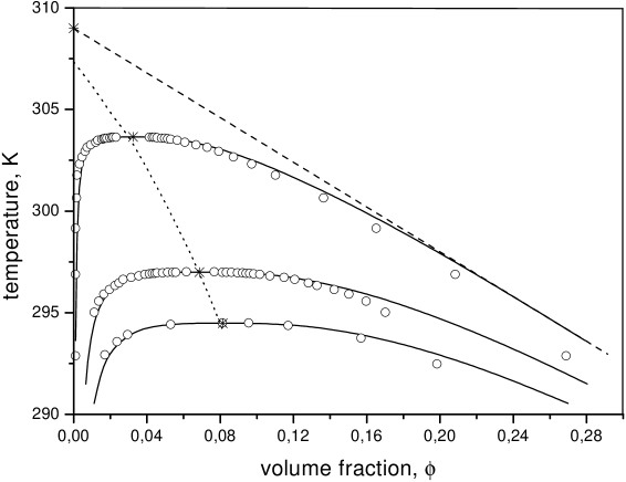
FIG. 2.: Coexistence-curve data for PS in cyclohexane [42, 43, 44] are shown together with the result of the renormalized crossover theory (full curves). The dotted curve represents Eq. (59) with $\Theta=307.25$ K. The critical demixing points and the coexistence-curve scaling value of $\Theta=309$ K are denoted by stars. An estimate for the limiting phase-separation boundary with $\phi_{{\rm sd}}/\phi_{{\rm c}}=3$ is shown by the dashed line.

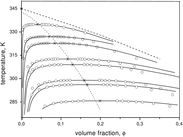
FIG. 3.: Coexistence-curve data for PS in methylcyclohexane [45] are shown together with the result of the renormalized crossover theory (full curves). The dotted curve represents Eq. (59) with $\Theta=342.75$ K. The critical demixing points and the coexistence-curve scaling value of $\Theta=345$ K are denoted by stars. An estimate for the limiting phase-separation boundary with $\phi_{{\rm sd}}/\phi_{{\rm c}}=3$ is shown by the dashed line.

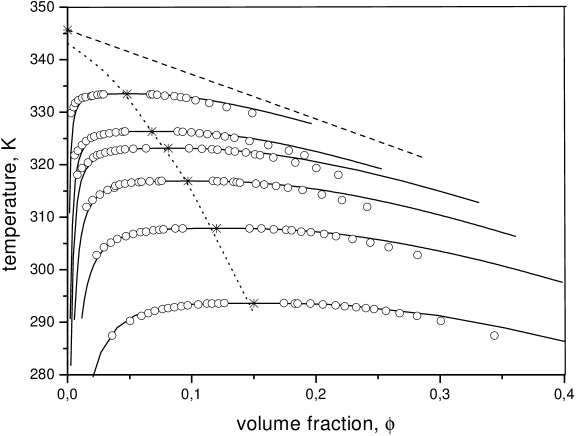
FIG. 4.: Coexistence-curve data for PMMA in $3$-octanone [46, 47] are shown together with the result of the renormalized crossover theory. The dotted curve represents Eq. (59) with $\Theta=343.15$ K. The critical demixing points and the coexistence-curve scaling value of $\Theta=345.65$ K are denoted by stars. An estimate for the limiting phase-separation boundary with $\phi_{{\rm sd}}/\phi_{{\rm c}}=3$ is shown by the dashed line.

Compared to other methods, that use mean-field extrapolations of the critical parameters $\phi_{{\rm c}}$ and $T_{{\rm c}}$ leading to values $\Theta=305.6$ - $308.4$ K (see Ref. [48] p. 163) for the system PS in cyclohexane, our value is at the upper end of the estimated range. This method of fitting the $\Theta$-temperature has the advantage, that no explicit $N$-dependence for $T_{{\rm c}}(N)$ needs to be assumed. The scaled data are displayed on a linear scale in Fig. 3 and in a logarithmic scale in Fig. 4. Note that the one data set of Ref. [46] with $M_{{\rm w}}=26,900,$ which is significantly off the scaling curve (see log plot), has also the largest polydispersity index $M_{{\rm w}}/M_{{\rm n}}=1.11$ of all samples. It is interesting to observe that the data for all three systems with good accuracy collapse onto a single scaling curve, as is suggested by the solution of the unrenormalized coexistence conditions (30) indicated by a dashed line in Figs. 3 and 4. This is not necessarily to be expected, since the critical renormalization introduces two additional parameters $\bar{u}$ and $\tilde{c}_{\rho}$ which may have different values for different solutes and solvents. One clearly sees, that the unrenormalized scaled coexistence curve fails to reproduce the proper Ising-type singularity (11) with $\beta=0.325$ close to the critical point, but instead has the mean-field exponent $\beta=1/2$. In our second step in fitting the data we remedy this deficiency by applying the renormalization procedure as outlined in Sec. III. Since the parameter $\bar{u}$ was already found to be close to unity in a recent evaluation of light-scattering data above $T_{{\rm c}}$ [18], and its variation does not affect the coexistence curves very much, we fixed it to $\bar{u}=1$, leaving $\tilde{c}_{\rho}$ as the only fit parameter of the crossover theory. The result of our fit with $\tilde{c}_{\rho}=1.6$ is displayed in Figs. 2-4 in terms of unscaled variables and in Figs. 5 and 6 in terms of scaled variables. Our scaled crossover formulation nicely reproduces the Ising singularity, but shows some deviations in the crossover region which cannot be removed by tuning $\tilde{c}_{\rho}$. One can think of a plethora of possible sources for such a deviation, since in our approach we neglected higher-order terms in expansions at several stages in our calculations. We truncated the virial expansion at order $\phi^{3}$, included only first-order perturbative corrections in $\lambda$ and $v$, and used the lowest-order approximations for the temperature dependence of $\lambda$ and $v$. The influence of higher-order terms in the expansion of the temperature dependence of $\lambda$ and $v$ and similarly of higher-order terms in the perturbation theory causes only a change of the scaling variable $\Delta\tilde{\lambda}$, that cannot account for the deviation. Note that both coexisting densities $\phi_{1}$ and $\phi_{2}$ of the renormalized fit are shifted to higher densities as compared to the experimental data. Higher-order terms in the virial expansion, like a negative $\phi^{4}$-term can induce a shift of both coexisting densities in the double-tangent construction (50) to lower values. Since we use the theory to volume fractions up to $\phi\leq 0.4$, it is likely that such higher-order terms in the virial expansion contribute to the observed deviations.

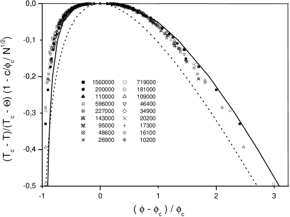
FIG. 5.: Linear scaling plot of phase-coexistence curves for PS in cyclohexane [42, 43, 44] (full symbols), PS in methylcyclohexane [45] (open symbols) and PMMA in $3$-octanone [46, 47] (open crossed symbols). The dashed curve represents the values calculated from the unrenormalized scaled free energy (29) and the full line represents the result of renormalized crossover theory with $\bar{u}=1$ and $\tilde{c}_{\rho}=1.6$.

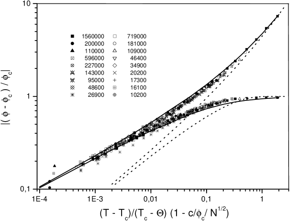
FIG. 6.: Logarithmic scaling plot of phase-coexistence curves for PS in cyclohexane [42, 43, 44] (full symbols), PS in methylcyclohexane [45] (open symbols) and PMMA in $3$-octanone [46, 47] (open crossed symbols). The dashed curve represents the values calculated from the unrenormalized scaled free energy (29) and the full line represents the result of renormalized crossover theory with $\bar{u}=1$ and $\tilde{c}_{\rho}=1.6$.

B Scaling of the critical parameters

In the previous section we assigned values for the $\Theta$-temperature that optimized scaling of the coexistence curves. An alternative procedure to estimate the $\Theta$-temperatures is by extrapolating $N\rightarrow\infty$ in accordance with Eqs. (58) and (59). The values thus obtained for $(\Theta-T_{{\rm c}})/\Theta$ are plotted in Fig. 7 as a function of $\phi_{{\rm c}}^{-3/11}N^{-7/11}$. The solid lines indicate the asymptotic linear relations in accordance with Eq. (58). The slope of this linear relation was found to be $2$ for PS in cyclohexane, $2.5$ for PS in methylcyclohexane and $3.5$ for PMMA in $3$-octanone. The resulting estimates for the $\Theta$-temperatures are $\Theta=307.25$ K for PS in cyclohexane, $\Theta=342.75$ K for PS in methylcyclohexane and $\Theta=343.15$ K for PMMA in $3$-octanone. They all lie about $0.7\%$ below the values found from coexistence-curve scaling. Those for polystyrene compare well with other extrapolations of critical-point data [48]. We believe that the origin of the discrepancy again lies in the neglect of higher-order terms in our calculations. To discriminate between the relations (57) - (59) we form a ratio $A$, by dividing the right-hand side of each equation by its left-hand side. The resulting ratio should be constant. The values of the ratio $A$ for Eqs. (57) - (59) and the three data sets are displayed in Fig. 8, with the left-most values being normalized to unity within each set and with an additive offset to separate the data sets. One clearly sees, that the unrenormalized prediction of Eq. (57) gives the worst fit and this cannot be improved by lowering the $\Theta$-temperature, since then the curves start bending upwards close to $\Theta$-temperature. The renormalized fits for PS in cyclohexane and PMMA in $3$-octanone are indeed constant within the scattering of the data, but the most precise data on PS in methylcyclohexane clearly show a residual slope which can be easily accounted for by introducing a correction $(\Theta-T_{{\rm c}})^{2}$. This, together with the mismatch to the $\Theta$-temperatures from coexistence-curve scaling, indicates the presence of second-order terms. Our fits for the critical-point scaling are included as dotted lines in Figs. 5-2. We also included the $\Theta$-temperatures obtained from coexistence-curve scaling and a guess for the limiting phase boundary $\phi_{{\rm sd}}$, assuming the ratio $\phi_{{\rm sd}}/\phi_{{\rm c}}=3$. Note that a value of $\phi_{{\rm sd}}/\phi_{{\rm c}}=5/2$ is not in accord with the experimental data unless one assumes the presence of large corrections to the asymptotic value. We think this is unlikely since the value of the ratio is not altered by the leading order of tricritical renormalization [27].

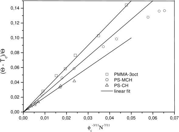
FIG. 7.: The reduced temperature difference between the critical point and the $\Theta$-point is plotted versus $\phi_{{\rm c}}^{-3/11}N^{-7/11}$. The symbols denote the critical parameter data for three experimental systems. The lines indicate the asymptotic linear approximation in accordance with Eq. (58).

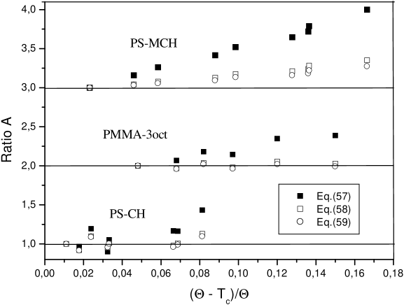
FIG. 8.: The ratio $A$ (right side / left side of Eqs. (57)-(59)) plotted against the reduced difference between the critical temperature and the $\Theta$-temperature. The experimental data for three different systems are separated by an offset of magnitude $1$.

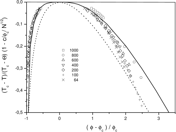
FIG. 9.: Linear scaling plot of simulated phase-coexistence curves [49] for self-avoiding walks with nearest-neighbor interaction on a simple cubic lattice. The dotted curve represents the values calculated from the unrenormalized scaled free energy (29) and the solid curve represents the renormalized crossover theory with $\bar{u}=1$ and $\tilde{c}_{\rho}=1.5$.

C Simulations

We have also analyzed a set of coexistence-curve data obtained from computer simulations of self-avoiding walks with attractive nearest-neighbor interaction on a simple cubic lattice [49] along the same lines as was done for the experimental coexistence-curve data in Sec. V A. We considered seven sets of coexistence-curve data with chain lengths ranging from $64$ to $1,000$ monomers. Figure 9 shows a linear scaling plot of the simulation data and Fig. 10 a logarithmic one. The optimal data collapse was obtained for $\Theta=3.754$, measured in units of the nearest-neighbor interaction energy, and $c=0.51$. The value for $\Theta$ again is $1\%$ higher than the best value $\Theta=3.717(2)$ obtained from extrapolation of $1/T_{{\rm c}}$ [27]. In general the quality of the data collapse is less satisfactory, compared to the experimental data. Especially on the semi-dilute branch the data for $N=800$ and $N=1,000$ deviate significantly from those for smaller chain lengths. One main difference between experiment and simulations is that the simulations were done in rather small boxes. These boxes were chosen to be at least four times larger than the maximum value of the radius of gyration. However, with the mean squared end-end distance of a random walk being a factor $\sqrt{6}$ larger, this still implies that a single polymer stretches over a significant portion of the box, causing finite-size effects. Also the rather small and varying total number of polymers, ranging between $80$ and $350$ for different simulations may cause problems in obtaining reliable bulk estimates, since large surface contributions are to be expected. On the other hand, we observe a clear breakdown of coexistence-curve scaling for the simulation data for the shorter chain lengths $8,16$ and $32$. This is to be expected, since we then reach volume fractions where our virial expansion is no longer accurate. Furthermore, the symmetric coexistence curve of the Ising model for $N=1$ cannot be scaled onto a asymmetric scaling curve with a finite reparametrization. The two fit parameters $\bar{u}$ and $\tilde{c}_{\rho}$ of our crossover theory are not sufficient to provide a decent fit to the scaling curve, probably due to the reasons already discussed for the fit of the experimental data. More work has to be invested in order to decide, whether the observed mismatch is due to a limitation of the coexistence-curve scaling or can be attributed to systematic deviations in the simulation data.

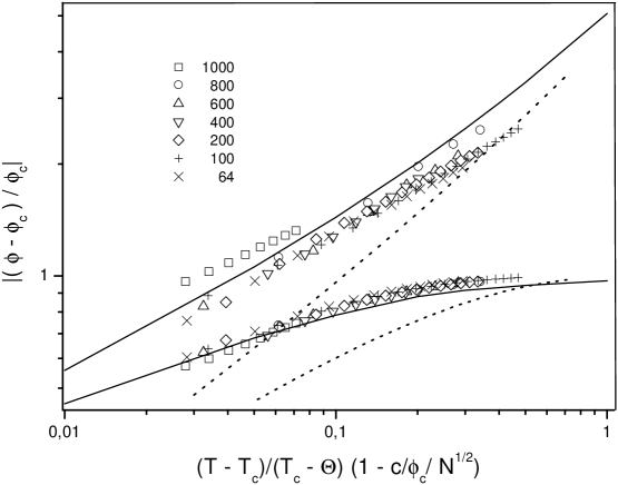
FIG. 10.: Logarithmic scaling plot of simulated phase-coexistence curves [49] for self-avoiding walks with nearest-neighbor interaction on a simple cubic lattice. The dotted curve represents the values calculated from the unrenormalized scaled free energy (29) and the solid curve represents the renormalized crossover theory with $\bar{u}=1$ and $\tilde{c}_{\rho}=1.5$.

VI Conclusion

We find that the scaling description for coexistence curves of polymer solutions, including first-order perturbative corrections, provides a decent collapse of the available experimental data onto a single scaling curve at fitted $\Theta$-temperatures which are systematically about $0.7\%$ higher than those obtained from an extrapolation of critical point data to infinite chain-length. Incorporation of the critical fluctuations via crossover RG theory leads to a decent description of the scaled coexistence curve by fitting essentially only one parameter $\tilde{c}_{\rho}=1.6$. We attribute the remaining deviations in the fit and the discrepancies in the $\Theta$-temperature estimates mainly to two approximations in our approach. First, we truncated the virial expansion after the $\phi^{3}$ term, neglecting higher-order terms that contribute at larger volume fractions, and will perturb the scaling description as they do in the Flory-Huggins model. Another source of corrections are higher-order terms in the temperature dependence of the bare parameters and higher-order corrections of perturbation theory, which have similar effects on the scaling variable $\Delta\tilde{\lambda}$. We find that both simulations and experiments are pointing towards an universal ratio $\phi_{{\rm sd}}/\phi_{{\rm c}}=3$, implying that $\phi_{{\rm c}}$ has to be calculated at constant chain length $N$ rather than at constant field $h_{2}$, which would lead to $\phi_{{\rm sd}}/\phi_{{\rm c}}=5/2$ in the Landau theory. The scaling description is less satisfactory for coexistence-curve data provided by simulations. Concerning the $\Theta$-temperature extrapolations we find from the simulation data the same pattern as for the experimental data, with the value of $\Theta$, obtained from the scaling description, being $1\%$ higher than the best value obtained from a extrapolation of $1/T_{{\rm c}}(N)$.

Acknowledgments

The authors acknowledge a fruitful collaboration with V.A. Agayan in an earlier stage of this research [25] and stimulating interactions with A. Z. Panagiotopoulos and B. Widom. The research has been supported by the Chemical Sciences, Geosciences and Biosciences Division, Office of Basic Energy Sciences, Office of Science, U.S. Department of Energy under Grant No. DE-FG-02-95ER-14509.

REFERENCES

- [1] C. M. Knobler and R. L. Scott, in: Phase Transitions and Critical Phenomena, Vol. 9, edited by C. Domb and J. L. Lebowitz, (Academic Press, New York, 1984), p. 163.
- [2] M. A. Anisimov, Critical Phenomena in Liquids and Liquid Crystals, (Gordon and Breach, Philadelphia, 1991).
- [3] P. G. de Gennes, Scaling Concepts in Polymer Physics, (Cornell University Press, Ithaca, NY, 1979).
- [4] P. G. de Gennes, J. Phys. (Paris) 39, L299 (1978).
- [5] P. G. de Gennes, J. Phys. (Paris) 36, L55 (1975).
- [6] M. E. Fisher, J. Stat. Phys. 75, 1 (1994).
- [7] J. des Cloizeaux, J. Phys. (Paris) 36, 281 (1975).
- [8] M. A. Moore, J. Phys. (Paris) 38, 265 (1977).
- [9] L. Schäfer and T. A. Witten, J. Chem. Phys. 66, 2121 (1977).
- [10] J. C. Wheeler and P. Pfeuty, J. Chem. Phys. 74, 6415 (1981).
- [11] M. J. Stephen, Phys. Lett. A. 53, 363 (1975).
- [12] B. Duplantier, J. Phys. (Paris) 43, 991 (1982).
- [13] J. Hager and L. Schäfer, Phys. Rev. E 60, 2071 (1999).
- [14] P. J. Flory, Principles of Polymer Chemistry, (Cornell University Press, Ithaca, NY, 1953), Ch. XIII., M. Huggins, J. Phys. Chem. 46, 151 (1942).
- [15] M. Doi, Introduction to Polymer Physics, (Clarendon Press, Oxford, 1996).
- [16] B. Widom, Physica A 194, 532 (1993).
- [17] Y. B. Melnichenko, M. A. Anisimov, A. A. Povodyrev, G. D. Wignall, J. V. Sengers, and W. A. Van Hook, Phys. Rev. Lett. 79, 5266 (1997).
- [18] M. A. Anisimov, A. Kostko, and J. V. Sengers, Phys. Rev. E 65, 051805 (2002).
- [19] V. A. Agayan , M. A. Anisimov, and J. V. Sengers, Phys. Rev. E 64, 026125 (2001).
- [20] A. A. Povodyrev, M.A. Anisimov, and J.V. Sengers, Physica A 264, 345 (1999).
- [21] Z. Y. Chen, P.C. Albright, and J. V. Sengers, Phys. Rev. A 41, 3161 (1990).
- [22] Z. Y. Chen, A. Abbaci, S. Tang, and J. V. Sengers, Phys. Rev. A 42, 4470 (1990).
- [23] L. Schäfer and T. A. Witten, J. Phys. (Paris) 41, 459 (1980).
- [24] L. Schäfer, Excluded Volume Effects in Polymer Solutions, (Springer, Heidelberg, 1999).
- [25] M. A. Anisimov, V. A. Agayan and E. E. Gorodetskii, JETP Lett. 72, 578 (2000).
- [26] S. Sarbach and M. E. Fisher, Phys. Rev. B 20, 2797 (1979).
- [27] H. Frauenkron and P. Grassberger, J. Chem. Phys. 107, 9599 (1997).
- [28] P. Grassberger, Phys. Rev. E 56, 3682 (1997).
- [29] J. F. Nicoll and P. C. Albright, Phys. Rev. B 31, 4576 (1985).
- [30] J. Zinn-Justin, Quantum Field Theory and Critical Phenomena, (Clarendon Press, Oxford, 1996).
- [31] C. Domb and M. S. Green (eds.), Phase Transitions and Critical Phenomena, Vol. 6 (Academic Press, New York, 1976).
- [32] S. Tang, J. V. Sengers, and Z. Y. Chen, Physica A 179, 344 (1991).
- [33] A. J. Liu and M. E. Fisher, Physica A 156, 35 (1989).
- [34] R. Guida and J. Zinn-Justin, J. Phys. A 31, 8103 (1998).
- [35] M. Campostrini, A. Pelisettimo, P. Rossi and E. Vicari, Phys. Rev. E 60, 3526 (1999).
- [36] S.-Y. Zinn and M. E. Fisher, Physica A 226, 168 (1996).
- [37] Y. Izumi and Y. Miyake, J. Chem. Phys. 81, 1501 (1984).
- [38] I. C. Sanchez, J. Phys. Chem. 93, 6983 (1989).
- [39] A. Kostrowicka Wyczalkowska, M.A. Anisimov, and J.V. Sengers, Fluid Phase Equilibria 158-160, 523 (1999).
- [40] I. D. Lawrie and S. Sarbach, in: Phase Transitions and Critical Phenomena, Vol. 9, edited by C. Domb and J. L. Lebowitz (Academic Press, New York, 1984), p. 1.
- [41] J. S. Hager, J. Phys. A 35, 2703 (2002).
- [42] M. Nakata, T. Dobashi, N. Kuwahara, M. Kaneko, and B. Chu, Phys. Rev. A 18, 2683 (1978).
- [43] M. Nakata, N. Kuwahara, and M. Kaneko, J. Chem. Phys. 62, 4278 (1975).
- [44] J. Kojima, N. Kuwahara, and M. Kaneko, J. Chem. Phys. 63, 333 (1975).
- [45] T. Dobashi, M. Nakata, and M. Kaneko, J. Chem. Phys. 72, 6685 (1980); ibid. 72, 6692 (1980).
- [46] K. Q. Xia, X.-Q. An, and W. G. Shen, J. Chem. Phys. 105, 6018 (1996).
- [47] K. Q. Xia, C. Frank, and B. Widom, J. Chem. Phys. 97, 1446 (1992).
- [48] K. Kamide and T. Dobashi, Physical Chemistry of Polymer Solutions, (Elsevier, Amsterdam, 2000).
- [49] A. Z. Panagiotoupoulos, V. Wong and M. A. Floriano, Macromolecules 31, 912 (1998).