Holstein polarons in a strong electric field: delocalized and stretched states

Abstract

The coherent dynamics of a Holstein polaron in strong electric fields is considered under different regimes. Using analytical and numerical analysis, we show that even for small hopping constant and weak electron-phonon interaction, the original discrete Wannier-Stark (WS) ladder electronic states are each replaced by a semi-continuous band if a resonance condition is satisfied between the phonon frequency and the ladder spacing. In this regime, the original localized WS states can become delocalized, yielding both ‘tunneling’ and ‘stretched’ polarons. The transport properties of such a system would exhibit a modulation of the phonon replicas in typical tunneling experiments. The modulation will reflect the complex spectra with nearly-fractal structure of the semi-continuous band. In the off-resonance regime, the WS ladder is strongly deformed, although the states are still localized to a degree which depends on the detuning: Both the spacing between the levels in the deformed ladder and the localization length of the resulting eigenfunctions can be adjusted by the applied electric field. We also discuss the regime beyond small hopping constant and weak coupling, and find an interesting mapping to that limit via the Lang-Firsov transformation, which allows one to extend the region of validity of the analysis.

I Introduction

Quantum electronic transport properties in semiconductor superlattices in high electric fields have been the subject of much interest in recent years. Experimental studies have reported interesting phenomena, such as Bloch oscillations and Wannier-Stark (WS) ladders. exp1 Moreover, a number of theoretical predictions have been made, including negative differential conductivity, con dynamical localization, dy and fractional WS ladders under DC and AC fields, fws to name a few.

One important issue for the dynamical behavior of a real system is the effect of electron-phonon interactions, and extensive research in this field has been reported. For example, Ghosh et al. and Dekorsy et al. studied coupled Bloch-phonon oscillations. blo The phonon-assisted hopping of an electron on a WS ladder was studied in [pho1, ]. A brilliant variational treatment of inelastic quantum transport was given in [tru, ], and anomalies in transport properties under a resonance condition were studied in [res, ]. Govorov et al. studied the optical absorption associated with the resonance of a WS ladder and the optical phonon frequency in a system. gov1 ; gov2 A similar and fascinating system of electron-phonon resonance in magnetic fields has also been studied extensively. mag

Much of the work in this area considers incoherent scattering of electrons by phonons, which is the relevant picture in systems at high temperature. In this paper, however, we report a study of the effects of coherent coupling of an electron to the phonons of the system, likely to be the relevant description at low temperatures. We concentrate on how the phonon coupling affects electron transport in high electric field, in a situation typically achieved in semiconductor superlattices, for instance, but also important for electrons in polymer chains, conwell and even perhaps reachable in a stack of self-assembled quantum dots. dots

Based on a Holstein model, holst typically used to describe the small polaron in molecular systems, we analyze the spectrum of the system and study its transport properties. We use here a non-perturbative description, which allows one to elucidate the effects of resonant and non-resonant phonon fields on the otherwise localized electrons residing in a WS ladder, for both weak and strong electron-phonon coupling. We find that for small hopping and coupling constant, an interesting regime results when two characteristic energy scales in the system coincide: the one corresponding to the energy spacing between the WS levels, and the other corresponding to the frequency of the phonons. In this resonant case, the problem is one of strong mixing between degenerate states with rather different properties. The result is a complex semi-continuous band structure replacing each of the original WS ladder ‘rungs’, where some of the electron states become delocalized, despite the strong electric field present. In this case, the phonons interacting with the electron provide delocalization, unlike the usual situation. Moreover, and in contrast to these extended states, ‘stretched polarons’ are highly degenerate and exhibit strongly localized electronic components, while the phonon component is in fact extended throughout the structure. When the system is away from the resonance condition, a deformed WS ladder will appear, with very interesting substructure. The electronic wave functions in this regime are all localized, but with a localization length that depends linearly on the degree of detuning.

In all phonon frequency regimes, the rich dynamical behavior of the system is due to (or reflected in) the near fractal structure of the spectrum. This, as we will discuss, has a direct connection to the Cayley tree structure of the relevant Hilbert space. This structure is of course contained in the Hamiltonian and reflected also in the structure of the eigenvectors.

We also extend our studies beyond the weak coupling and small hopping constant regime, via a Lang-Firsov transformation. This results in an interesting mapping of the problem from the strong coupling to the weak limit, and allows one to extend the results for a wider parameter range. A first report of the resonant case in the weak coupling regime has been published. EPLus Here, we give a detailed theory of such states, including both resonant and non-resonant cases, and present the strong coupling interaction regime.

In what remains of the paper, we give in section II a description of the model used and the relevant Hilbert space in the problem. Section III contains a complete analysis of the resulting spectrum for small hopping constant and weak phonon coupling. The extension beyond that regime is given in section IV. A final discussion is presented in section V.

II Description of the model

We consider the Holstein model, holst which describes an electron in a one-dimensional tight-binding lattice, interacting locally with dispersionless optical phonons. Moreover, the system is subjected to a strong static electric field. The Hamiltonian is then given by

$$H_{0} = \sum_{j}\varepsilon_{j}c^{+}_{j}c_{j}+t\sum_{j}(c_{j}^{+}c_{j+1}+c^{+}_{j+1}c_{j})$$ (1)

$$+ \omega\sum_{j}a_{j}^{+}a_{j}+\gamma\sum_{j}c_{j}^{+}c_{j}(a_{j}^{+}+a_{j})\,,$$

where $t$ is the electron hopping constant, $\omega$ the phonon frequency (or energy, with $\hbar=1$), $\gamma$ the electron-phonon coupling constant, $\varepsilon_{j}=-edEj\equiv-j\Delta$ the site energy, $E$ the electric field, and $d$ is the lattice constant. It is known that a series of localized WS states will form in a strong field ($\Delta=edE\gg t$), in the absence of interactions between electron and phonons. Within tight-binding theory, the eigenvalues and eigenfunctions of these WS states are, respectively $\varepsilon_{j}=-edEj$, and

$$\begin{array}[]{l}|\phi_{j}\rangle=\sum_{i}J_{i-j}(2t/edE)|i\rangle\,,\end{array}$$ (2)

where $J_{l}$ is the $l$-th order Bessel function. The WS states are localized states with characteristic length $2t/eE$.

It is helpful to introduce creation and annihilation operators for WS states as

$$\begin{array}[]{l}d_{j}=\sum_{i=-\infty}^{\infty}J_{i-j}(2t/edE)\,c_{i}\,.\end{array}$$ (3)

It is easy to show that this transformation is canonical, $\{d^{+}_{i},d_{j}\}=\delta_{ij}$, and that the Hamiltonian can be written in terms of $d_{j},d^{+}_{j}$ as

$$H_{0} = -\sum_{j}j\Delta d_{j}^{+}d_{j}+\sum_{j}\omega a_{j}^{+}a_{j}$$

(4)

$$+ \gamma\sum_{j,i,i^{\prime}}J_{j-i}J_{j-i^{\prime}}(a_{j}+a_{j}^{+})d_{i}^{+}d_{i^{\prime}}\,.$$

In the case of strong electric field (or small hopping constant, $2t/\Delta\ll 1$) in which we concentrate in this section, the Hamiltonian can be simplified as

$$H = -\sum_{j}j\Delta d_{j}^{+}d_{j}+\omega\sum\limits_{j}a_{j}^{+}a_{j}+\gamma\sum\limits_{j}d_{j}^{+}d_{j}(a_{j}^{+}+a_{j})$$

$$- \lambda\sum_{j}(a_{j}+a_{j}^{+}-a_{j+1}^{+}-a_{j+1})(d_{j}^{+}d_{j+1}+d_{j+1}^{+}d_{j})\,,$$

where the effective coupling constant is now

$$\lambda=\gamma t/\Delta\,.$$ (6)

From (LABEL:H), one can see phonon-assisted hopping between the WS states quite clearly, so that in fact the phonons introduce delocalization of the WS electrons. The Hamiltonian (LABEL:H) is similar to that in [gov1, ], but there are some differences. In the current model, when an electron jumps from one site to the next, it can not only emit (or absorb) a phonon on (from) its site, but also onto (from) the nearby site. This more natural description also produces a large difference on the relevant Hilbert spaces. The dimension of the relevant Hilbert space in our case is $2^{n}-1$, where $n$ is the number of local sites in the chain, while the size is $n$ for the model in [gov1, ]. As we will see, the resulting energy spectrum and other physical quantities show quite a rich behavior.

Let us consider the process of an electron jumping between sites while creating or annihilating phonons in its neighborhood. For example, for a chain of three sites, $n=3$, the hopping of the electron from the first site will connect the states $|1;000\rangle$, $|2;010\rangle$, $|2;100\rangle$, $|3;011\rangle$, $|3;101\rangle$, $|3;020\rangle$, and $|3;110\rangle$. Here a vector is expressed as $|j;...m_{0},m_{1},...\rangle$, where $j$ is the electron position, and $m_{k}$ refers to the number of phonons on site $k$. It is interesting to see that the connectivity of this portion of Hilbert space has the structure of a Cayley tree, or a Bethe lattice.car Under the condition of resonance, i.e., $\Delta=\omega$, all the states above for $n=3$ have the same energy. The off-diagonal matrix elements therefore break the degeneracy and allow level mixing, and one can expect that some kind of band may form in the limit of large $n$. As we will see later on, and in contrast to the resonant case, the spectrum in off-resonance is still composed of ladders although with a complex structure. note

In the basis we list above, the Hamiltonian for $n=3$ takes the form

$$\begin{array}[]{l}H=\left(\begin{array}[]{ccccccc}-\Delta&\lambda&-\lambda&0&0&0&0\\ \lambda&-2\Delta+\omega&0&\lambda&0&-\sqrt{2}\lambda&0\\ -\lambda&0&-2\Delta+\omega&0&\lambda&0&-\lambda\\ 0&\lambda&0&-3\Delta+2\omega&0&0&0\\ 0&0&\lambda&0&-3\Delta+2\omega&0&0\\ 0&-\sqrt{2}\lambda&0&0&0&-3\Delta+2\omega&0\\ 0&0&-\lambda&0&0&0&-3\Delta+2\omega\end{array}\right).\end{array}$$ (7)

A direct consequence of the Cayley tree connectivity of the near degenerate basis is that the Hamiltonian (7) is constructed by diagonal block matrices for ever larger $n$ (of sizes 1, 2, 4, …, 2^n-1), and mixed by off-diagonal matrix elements proportional to $\lambda$. One can see that in the resonant case, all diagonal elements are given by $-\Delta$, corresponding to the degenerate manifold. Notice also that the off-diagonal elements are given by $\pm\lambda$, except for a few sporadic elements which appear as $\sqrt{2}\lambda$, associated with higher number of phonons in a site, such as the state $|3;020\rangle$ in this case. This nearly self-similar structure appears for all values of $n$. We expect then that there would be little change in the physical properties in the large $n$ limit if we replace $-\sqrt{2}\lambda$ in those few off-diagonal spots with $-\lambda$. This will be confirmed by our numerical calculation, as we will see below. After the substitution, the new symmetrized Hamiltonian $H_{sym}$ takes a full self-similar form, and allows one to exactly solve analytically the eigenvalue problem, and better understand the physics of the system. Much of the behavior of $H_{sym}$ remains in the actual system described by $H$.

III Small hopping and weak coupling regime

Let us consider the eigenvalue problem for the Hamiltonian $H_{sym}$, defined as that in (7), except that the elements $-\sqrt{2}\lambda$ are replaced by $-\lambda$. By using the block decomposition formula

$$\begin{array}[]{l}\det\left(\begin{array}[]{cc}A&B\\ C&D\end{array}\right)=\det(D)\det(A-BD^{-1}C),\end{array}$$ (8)

we find that the eigenvalues of the Hamiltonian $H_{sym}$ are determined by the equation

$$\begin{array}[]{l}\varepsilon_{0}^{N/2}\varepsilon_{1}^{N/4}\varepsilon_{2}^{N/8}...\varepsilon_{n-1}^{1}=0\,,\end{array}$$ (9)

where $N=2^{n}$, $\varepsilon_{0}=\varepsilon-t_{n}$, $\varepsilon$ is the energy eigenvalue, $t_{k}$ is defined by

$$\begin{array}[]{l}t_{k}=(n-k)(\omega-\Delta)-\omega\,,\end{array}$$ (10)

and

$$\begin{array}[]{l}\varepsilon_{k+1}=\varepsilon-t_{k}-\frac{\displaystyle 2\lambda^{2}}{\displaystyle\varepsilon_{k}}\,.\end{array}$$ (11)

Then, $\varepsilon_{k}$ can be written as a continuous fraction in $k$ steps

$$\begin{array}[]{l}\varepsilon_{k+1}=\varepsilon-t_{k}-\frac{\displaystyle 2\lambda^{2}}{\displaystyle\varepsilon-t_{k-1}-\frac{\displaystyle 2\lambda^{2}}{\displaystyle\varepsilon-t_{k-2}-\frac{\displaystyle 2\lambda^{2}}{\displaystyle...}}}\,.\end{array}$$ (12)

III.1 Resonant regime ($\Delta=\omega$)

In this case, $t_{k}=0$ (after a constant energy shift of $\omega$ is made), we obtain the eigenvalues of $H_{sym}$ as

$$\begin{array}[]{l}\varepsilon_{k,j}=2\sqrt{2}\lambda\cos\left(\frac{\displaystyle j\pi}{\displaystyle k+1}\right)\,,\end{array}$$ (13)

where $k=1,2,...,n$, and $j=1,...,k$. The asymptotic bandwidth of the spectrum is therefore given by $4\sqrt{2}\lambda$. Notice that this behavior is similar to that of a system in magnetic fields. In that case, the electron-phonon interaction breaks the degeneracy (under the condition of magnetic resonance) and leads to a “resonance splitting.” In that case, the splitting is $\propto\alpha^{2/3}$ for a three dimensional system, and $\propto\alpha^{1/2}$ for a two dimensional system, where $\alpha$ is the Frohlich electron-phonon coupling constant. mag

Let us consider the question of eigenvalue degeneracy by solving $\varepsilon^{N/2}_{0}\varepsilon^{N/4}_{1}\varepsilon^{N/8}_{2}\varepsilon^{N/16}_{3}=0$, which will provide us with a good estimate in the large $N$ limit. After some algebra, one obtains for the eigenvalue equation,

$$\varepsilon^{5N/16}(\varepsilon^{2}-2\lambda^{2})^{N/8}(\varepsilon^{2}-4\lambda^{2})^{N/16}$$ (14)

$$\times (\varepsilon^{4}-6\varepsilon^{2}\lambda^{2}+4\lambda^{4})^{N/16}=0\,.$$

We then have eigenvalues $\varepsilon=0$, $\pm\sqrt{2}\lambda$, $\pm 2\lambda$, and $\pm\lambda\sqrt{3\pm\sqrt{5}}$, with respective degeneracies of $5N/16$, $N/8$, $N/16$, and $N/16$. Higher order polynomials would slightly improve the degeneracy estimate for successively higher eigenvalues.

Our numerical results for the eigenvalues of $H_{sym}$, Fig. 1, and $H$, Fig. 2, exhibit very similar characteristics, as expected. The different panels in these figures show spectra for $n=8$, 9, and 11. One can see that the main structure of the spectra changes little with increasing $n$, although finer structure appears for higher $n$, filling to some extent the gaps of the previous structure. Our analytical results match exactly those of Fig. 1. The self-similar structure of the spectrum is the manifestation of such symmetry in $H_{sym}$. One can see that the original highly degenerate manifold is broadened into a semi-continuous band by the off-diagonal mixing elements of $H_{sym}$. Notice however that large residual degeneracies remain at the center of the band, and other symmetrical values, as described above by Eq. (14).

The structure of the full Hamiltonian $H$ is shown in Fig. 2, which still maintains a nearly self-similar structure, despite the sporadic $-\lambda\sqrt{2}$ ‘asymmetrical’ terms. Notice however that the degeneracy at $\varepsilon=0$ and other ‘plateau values’ is not exact here, but only seen as a slight break (or slope) of each plateau.

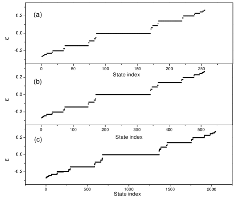
Figure 1: Energy spectra for fully self-similar $H_{sym}$ for systems with different lattice size, (a) $n=8$, (b) $n=9$, and (c) $n=11$. Notice the clear fractal structure of spectra, as anticipated from the structure of $H_{sym}$. Increasing $n$ produces finer scale structure in the gaps. Here $\Delta=\omega=1$, and $\lambda=0.1$, so that the asymptotic bandwidth is $4\sqrt{2}\lambda=0.5657$.

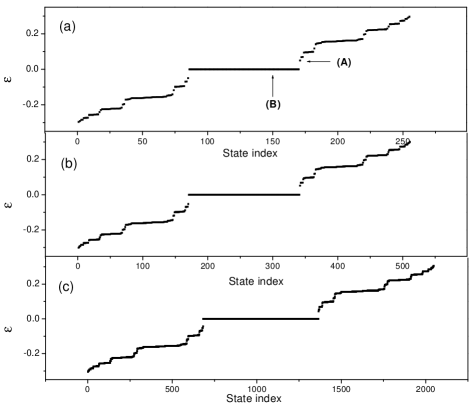
Figure 2: Energy spectra for $H$ of systems with different lattice size, (a) $n=8$, (b) $n=9$, and (c) $n=11$. Notice the approximate fractal structure of the spectra. Increasing $n$ gives similar structure. Here $\Delta=\omega=1$, $\lambda=0.1$, and the bandwidth slightly increases from one panel to the next. A and B labels in panel (a) indicate states described in Fig. 4 and 5.

Figure 3 compares the results for the bandwidth of $H$ and $H_{sym}$ from both analytical and numerical results. Notice that $4\sqrt{2}\lambda$ is the asymptotic (large $n$) analytical result from Eq. (13), for $H_{sym}$. We see in Fig. 3 that the numerical results for the bandwidth of $H_{sym}$ converge quickly to the analytical prediction. Similarly, the numerically obtained bandwidth of $H$ is only slightly larger than the bandwidth of $H_{sym}$, and clearly has also a finite asymptotic value. This is an interesting feature of $H$, that although one has large Hilbert space dimension $N-1=2^{n}-1$ (= 2047 for n=11, for example), one obtains a finite bandwidth. This is of course also associated with the fact that there are large degeneracies in the energy spectra, which increase with $N$ (see Eq. 14).

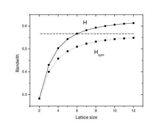
Figure 3: Bandwidth results for $\lambda=0.1$ and different values of $n$. The asymptotic bandwidth for $H_{sym}$ is $4\sqrt{2}\lambda=0.5657$, shown as dashed line. We see that bandwidth for $H$ is $W\gtrsim 6\lambda$.

To get better understanding of the physics, we show characteristic electron probabilities, as well as phonon spatial distributions, for different eigenstates in Fig. 4 and 5. The electronic probability function is given by

$$\begin{array}[]{l}P_{\nu}(j)=\langle\Psi_{\nu}|d^{+}_{j}d_{j}|\Psi_{\nu}\rangle=\sum_{\{m\}}|C^{\nu}_{j,\{m\}}|^{2}\,,\end{array}$$ (15)

where the coefficients in the last expressions are obtained from the diagonalization of $H$, so that the eigenvectors are given by

$$\begin{array}[]{l}|\Psi_{\nu}\rangle=\sum_{j,\{m\}}C^{\nu}_{j,\{m\}}\,|j;\{m\}\rangle\,,\end{array}$$ (16)

for each $\nu$-eigenstate. Similarly, the corresponding phonon spatial distribution is given by

$$\begin{array}[]{l}N_{\nu}(j)=\langle\Psi_{\nu}|a^{+}_{j}a_{j}|\Psi_{\nu}\rangle=\sum_{l,\{m\}}|C^{\nu}_{l,\{m\}}|^{2}m_{j}\,,\end{array}$$ (17)

for each eigenstate. These two spatial distribution functions give us an idea of how the two different components of each state are related to one another. These functions are a projection of the rather subtle coherent interactions (or mixtures) between the electron and phonon subsystems. One can see in Fig. 4a that for the non-degenerate state A in Fig. 2a, the electron is extended throughout the $n=8$ lattice. At the same time, the phonon amplitude is also extended along the lattice, and one can picture the phonon ‘cloud’ as ‘surrounding’ the electron all along in Fig. 4b, effectively describing a ‘tunneling polaron’. In contrast, the degenerate state B at $\varepsilon=0$ in Fig. 2a, has its electron component highly localized at the right end of the lattice, Fig. 5a, while the phonon cloud is away, Fig. 5b, and nearly ‘detached’ from the electron. One can describe this as a ‘stretched polaron’ (a precursor of the polaron dissociation predicted at high fields in polymer systems conwell ).

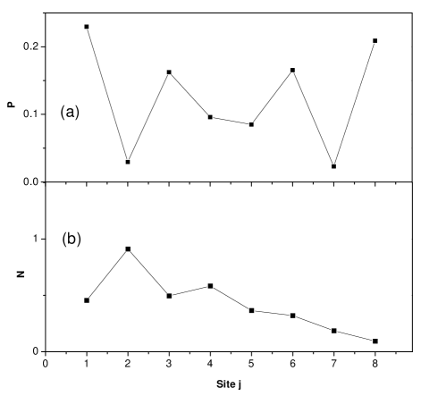
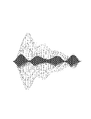
Figure 4: (a) Electron probability $P(j)$ for each site $j$, and (b) spatial distribution of phonons $N(j)$ for state labelled A in Fig. 2a. Large electron amplitude and phonon number throughout describe an extended, delocalized polaron, jointly illustrated in the composite figure at bottom.

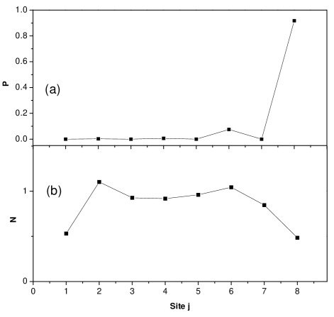
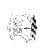
Figure 5: (a) Electron probability $P(j)$ for each site $j$, and (b) spatial distribution of phonons $N(j)$ for state labelled B in Fig. 2a. Electron is localized at right end of the chain, while phonons lie throughout, yielding a stretched polaron, illustrated at bottom figure.

Although by definition the electronic distribution function $P_{\nu}$ is normalized to unity, the phonon function $N_{\nu}$ is not necessarily so, since the electron can create and absorb phonons as it propagates up and down the lattice. This difference in phonon content for each state can be seen by comparing Fig. 4b, and 5b, as the total phonon number is clearly larger in the latter (stretched polaron) case. To study this feature throughout the spectrum, we show in Fig. 6 the total average phonon number of all states in the chain $n=8$. One can see clearly that states at the center of the band ($\varepsilon\approx 0$) have many more phonons ($\approx 7=n-1$) than the rest. An estimate for the average number of phonons for different states can be obtained by the following argument. The average phonon number is given by $\langle N_{\nu}\rangle=\sum_{i}P_{\nu}(i)m_{i}$. For an extended state, $P_{\nu}\simeq 1/n$, for a chain of $n$ sites. A state with an electron at site $i$ can be obtained by the electron hopping $i-1$ steps from the first site, while emitting $m_{i}\approx i-1$ phonons in the process. For extended states, this yields $\langle N\rangle\simeq\sum_{i}(i-1)/n=(n-1)/2$, which matches well the numerical results in Fig. 6, where the most extended states have $\langle N\rangle\simeq 3.5$ (such as the state labelled A). In contrast, an electron localized at site $n$, as B in Fig. 6, has emitted $n-1$ phonons in the process, just as one finds in the exact calculation.

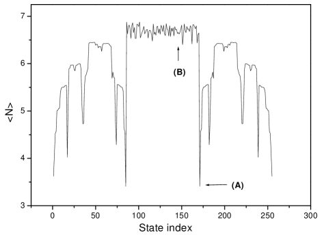
Figure 6: Total average phonon number for each eigenstate in Fig. 2a. Higher value plateaus are associated with the more localized electronic amplitudes, such as state B. Lowest phonon counts correspond to extended electronic states, such as A.

III.1.1 Transport through structure

We should emphasize that the properties illustrated in Fig. 4 and 5 are quite generic: states in one of the highly (nearly) degenerate levels show different degrees of electron localization and an abundance of phonons, in a stretched polaron configuration. In contrast, states with non-degenerate companions are delocalized polarons throughout the chain with low phonon content. Even though is the presence of phonons which delocalizes the electron (in the sense of the original WS ladder), we obtain that the localized electrons are accompanied by many phonons, reminiscent of the self-localized polarons when the coupling is strong.

The rather complicated behavior of the states would of course be reflected in various properties of the system. Let us focus here on what one could measure if electrons where injected from one end of the chain and were collected out of the other end. This is motivated by the ability to carry out just such experiments under strong electric fields in semiconductor superlattices, as well as in other systems. The transport properties provide information about the density of states in the structure and the spatial charge distribution of the different states (for optical response, see [EPLus, ]). The contribution of various eigenstates to the charge transport can be described by the quantity

$$\begin{array}[]{l}D_{\nu}=P_{\nu}(1)P_{\nu}(n)\,,\end{array}$$ (18)

since the tunneling amplitude is proportional to the density of states in the leads and the wavefunction amplitudes at both ends of the structure (the site $j=1$ and $j=n$). tul In fact, the tunneling probability can be calculated from the $S$-matrix formalism as $|T|^{2}$, where $T=\langle\varepsilon_{f},R|S|\varepsilon_{i},L\rangle$. Here $R$ and $L$ refer to the right and left leads. In the wide band limit,

$$T \propto \Gamma\int dt_{1}dt_{2}e^{i(\varepsilon_{f}t_{2}-\varepsilon_{i}t_{1})}\langle n|G^{R}(t_{2}-t_{1})|1\rangle$$ (19)

$$= \sum_{\nu}\Gamma\langle n|\nu\rangle\langle\nu|1\rangle\delta(\varepsilon_{f}-\varepsilon_{i})\,,$$

where $\Gamma$ describes the electron interaction with contacts, and $G^{R}$ is the retarded Green function connecting both ends of the structure ($j=1$ and $j=n$). We see then that the quantity $D_{\nu}=|\langle n|\nu\rangle\langle\nu|1\rangle|^{2}\propto|T|^{2}$ is directly involved in the tunneling probability. Figure 7a shows the density of states and 7b shows the quantity $D_{\nu}$ for the system with $n=8$. We can see that all the states at the center of the band contribute zero to the transport amplitude through the chain, and this behavior is exhibited by all the high peaks in the DOS. This is clearly consistent with the spatially localized charge nature of the highly degenerate states. On the other hand, $D$ shows large values for states ‘in the gaps’, confirming in fact that the non-degenerate states in the spectrum have an extended nature. The variations shown in $D$ would then be reflected in strong amplitude modulations within each of the phonon replicas in tunneling experiments, exp2 whenever the resonance regime is reached.

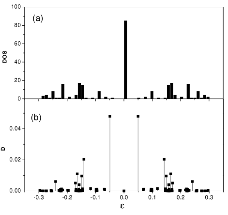
Figure 7: (a) Density of states, and (b) tunneling probability function $D_{\nu}$ for $n=8$ system.

III.2 Non-resonant regime ($\Delta\neq\omega$)

By studying the equivalent continuous fraction (12) for the non-resonant regime, we find that the spectrum for this case is quite different from that under resonance. For the case of small coupling constant, i.e., $\lambda/\omega\ll 1$, and $\lambda/\Delta\ll 1$, the unperturbed spectrum is a series of ladder levels $\varepsilon_{j}=-(\omega-\Delta)j$ ($j=1,...,n$) instead of the degenerate manifold in the degenerate case. Notice that the spacing between the ladders is given by the detuning, $\Delta^{\prime}\equiv|\omega-\Delta|$, instead of the original WS ladder energy. The correction introduced by the interaction breaks some of the detuned ladder degeneracies and gives some substructure to the ladder. Solving the first three factors, $\varepsilon_{0}^{N/2}\varepsilon_{1}^{N/4}\varepsilon_{2}^{N/8}=0$, to second order, $\lambda^{2}$, we find that the spectrum is a series of states with energies $n\Delta^{\prime}$, $n\Delta^{\prime}+2\lambda^{2}/\Delta^{\prime}$, $(n-1)\Delta^{\prime}$, $(n-1)\Delta^{\prime}-2\lambda^{2}/\Delta^{\prime}$, etc., with respective degeneracies $N/4$, $N/4$, $N/8$, $N/8$, etc. Notice that here the electron-phonon produces level splittings $\sim\lambda^{2}$, unlike the resonant case where the splitting (bandwidth) is linear in $\lambda$. The problem is also solved numerically and we show the resulting spectra in Fig. 8, for both $H$ (Fig. 8a), and $H_{sym}$ (Fig. 8b). Our analytical results match the numerical results for $H_{sym}$ quite well. We notice again that there are only small differences between the spectra of $H$ and $H_{sym}$.

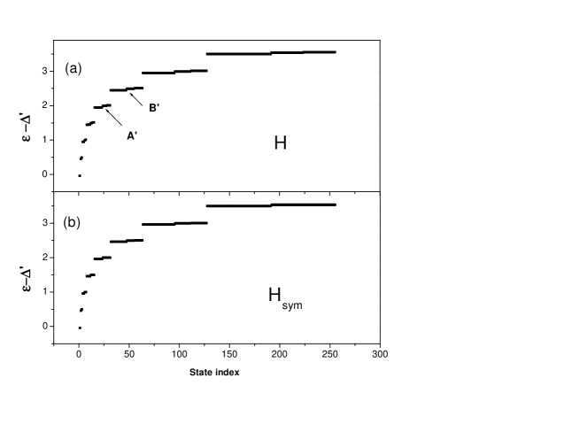
Figure 8: Energy spectra for system with lattice size $n=8$. (a) For full Hamiltonian $H$, and (b) for $H_{sym}$. Here $2\Delta=\omega=1$, and $\lambda=0.1$. A’ and B’ states are shown in Fig. 9.

Figure 9a, shows the electron probability for different states in the spectra, labelled A’ and B’ in Fig. 8a. Figure 9b shows the distribution of phonons for the same states. It is apparent that the electron wave function is localized, and separated from its phonon cloud. The two states only differ, basically, on which site to be localized about (as one would expect from their position in different ‘rungs’ in the ladder in Fig. 8a). In fact, the different states in the $\Delta^{\prime}$ ladder are associated with different lattice sites (the highest rung states at $\varepsilon\simeq n\Delta^{\prime}$ being localized at $j\simeq n$). We also show in Fig. 10 the average phonon number per state for the entire spectrum. The structure of this figure is quite different from that in Fig. 6, as they reflect dramatically different dynamical behavior. A phonon counting argument as the electron hops and emits phonons can explain the average number of phonons in the different states in Fig. 10, although clearly here it produces a nearly negligible mixing of states ($\sim\lambda^{2}$).

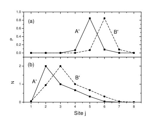
Figure 9: (a) Electron probability $P(j)$ for each site $j$ for states A’ and B’ indicated in Fig. 8a. (b) Corresponding phonon distributions $N(j)$.

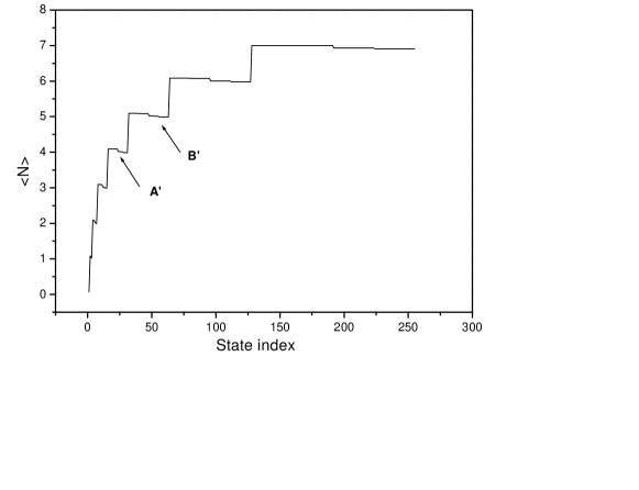
Figure 10: Total phonon number for each eigenstate in the non-resonant regime, as in Fig. 8.

One can further explore the extent of the localization nature of the eigenstates. In Fig. 11, we show the electronic probabilities of state (A’) for various $\Delta^{\prime}$ (or electric field) values. We might expect that the localization length would be $2\lambda/\Delta^{\prime}$, like the localization length for the original WS state is $2t/\Delta$. This simple expectation is confirmed by numerical calculations, as seen in Fig. 12, where the solid line shows the $2\lambda/\Delta^{\prime}$ dependence, and the dots indicate the localization length for states of various $\Delta^{\prime}$ [the localization length $L$ is extracted from a fit to an exponential amplitude drop about its central site, $e^{-|x|/L}$]. One would in fact expect that the manifestation of localization in real space (and energy) would be susceptible to be measured via Bloch oscillations, just as in a typical WS ladder. In this case, however, the frequency of Bloch oscillations is $\Delta^{\prime}$, and not $\Delta$. Thus the electron-phonon interaction changes the frequency of Bloch oscillations, and this effect may be possibly observed in experiment.

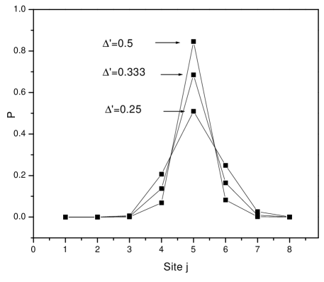
Figure 11: Electron probability $P(j)$ for state A’ in Fig. 8a for various detuning values $\Delta^{\prime}$.

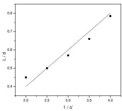
Figure 12: Relation between localization length $L$ and $1/\Delta^{\prime}$. Solid line shows $L/d=2\lambda/\Delta^{\prime}$ dependence, while the dots show value of $L$ obtained from fit of functions in Fig. 11 to the form exp$(-|x|/L)$.

From the discussion, it is clear that the eigenstates are localized in the non-resonant regime. As such, they contribute little to transport across the chain. One can easily calculate the quantity $D_{\nu}$ as before. As expected, the value of $D_{\nu}$ is very small ($<10^{-12}$) for every state, and very different from the resonant case. This behavior (not shown), is completely consistent with the localized nature of the eigenstates. Thus, we see that in this case the dominant conduction behavior, if any, would be thermally activated hopping conduction, instead of band conduction.

IV Beyond small hopping and weak coupling regime

All the discussions so far have been focused on the Hamiltonian $H$ (or $H_{sym}$), valid only under the condition of small hopping constant $t/\Delta\ll 1$. In this section we extend our discussion beyond this regime, which in principle may be relevant, depending on different system parameters.

We use the Lang-Firsov canonical transformation $H^{*}=e^{S}H_{0}e^{-S}$, where $S=-g\sum_{j}c_{j}^{+}c_{j}(a_{j}-a_{j+1})$, and $g=\gamma/\omega$. The transformed Hamiltonian takes the form

$$H^{*} = \sum_{j}\varepsilon_{j}c_{j}^{+}c_{j}+\omega\sum_{j}a_{j}^{+}a_{j}-g^{2}\omega c_{j}^{+}c_{j}$$

$$+ te^{-g^{2}}\sum_{j}[c_{j+1}^{+}c_{j}e^{g(a^{+}_{j+1}-a_{j}^{+})}e^{-g(a_{j+1}-a_{j})}+h.c.]\,.$$

One can see that this Hamiltonian is suitable for studying strong coupling dynamics. As in the case of $H$, we use the operators for WS ladder states, $d^{+}_{j}$. Then the Hamiltonian can be rewritten in the form

$$\begin{array}[]{l}\tilde{H}=-\sum_{j}(g^{2}+j)\Delta d_{j}^{+}d_{j}+\omega\sum_{j}a_{j}^{+}a_{j}+gt^{\prime}J^{2}_{o}(2t^{\prime}/\Delta)\sum_{j}[(a_{j+1}-a_{j+1}^{+}-a_{j}+a_{j}^{+})(d_{j}^{+}d_{j+1}-d_{j+1}^{+}d_{j})]\,,\end{array}$$ (21)

where $t^{\prime}=te^{-g^{2}}$. We see then that the effective hopping constant $t^{\prime}$ becomes smaller than $t$. Thus the problem can be mapped to that in the previous section, with effective hopping constant $t^{\prime}$, and effective coupling constant $\lambda^{\prime}$,

$$\begin{array}[]{l}t^{\prime}=te^{-g^{2}}\,,\quad{}\quad{}\lambda^{\prime}=gt^{\prime}J_{0}^{2}(2t^{\prime}/\Delta)\,.\end{array}$$ (22)

It is clear that $\lambda^{\prime}\rightarrow 0$, when $g\rightarrow 0$, as expected, and the spectrum is the discrete WS ladder in the absence of electron-phonon interaction. Moreover, one can see that for weak coupling, the bandwidth $W\simeq 6\lambda^{\prime}$ is proportional to $g$, just as in the situation discussed in III.A (see Fig. 3). Beyond the weak coupling and small hopping regime, however, $W$ and $\lambda^{\prime}$ have a nonlinear dependence on $g$. Figure 13 shows the coupling constant dependence of the bandwidth $W$ for the resonant and stronger coupling limit, $\Delta=\omega=t=1$. Notice that the bandwidth $W\simeq 1$ for $\gamma\gtrsim 0.6$. At this coupling, the bands in neighboring WS rungs will begin to overlap (and interband terms would need to be considered). It is clear that these corrections to the dependence of $W$ appear also as function of $t$, $\Delta$, and/or $\omega$.

Similar discussions are also relevant in the off-resonant case. For example, since the localization length is proportional to $2\lambda^{\prime}/\Delta^{\prime}$ (section III.B), there is also a correction to the simple relation $L\propto 2\lambda/\Delta^{\prime}$, when $t$ and/or $g$ are not small. For example, with increasing coupling constant, the correction to the ladder $\sim 2{\lambda^{\prime}}^{2}/\Delta^{\prime}$ may become comparable with the spacing between the detuned ladder levels $\Delta^{\prime}$. In that case, the ladder structure for the off-resonance case will also disappear. In this situation, the electron can also become delocalized, even if in the non-resonant regime, but due to the strong coupling $\gamma$.

It is interesting to compare our results to those of Bonca and Trugman,tru as one goes from the weak to the strong tunneling regime. These authors found by numerical calculation of the drift velocity that for small electron-phonon coupling, there are energies where the electron cannot propagate. In our approach, this corresponds to the formation of the quasi-continuous band for each of the WS ladders. The electron cannot propagate when its energy lies in the band gap. However, with increasing coupling constant, the band gap will disappear because of the overlap of subsequent bands. More quantitatively, let us consider the case $t=\omega=1$ (as the parameters in [tru, ]). Since the hopping constant is large, one needs to adopt the formalism in this section. As seen in Fig. 13, the bandwidth increases with increasing coupling constant, producing band overlap for large enough $\gamma$. This vanishing of the gaps as a function of $\gamma$ would coincide with the resumption of particle drift in the system. Just such behavior was found numerically in [tru, ], and one can now explain it in terms of the level structure of the system. It is also interesting to notice that the overall envelope seen in $D_{\nu}$ is similar to that of the drift velocity: small at the center and edge of each band, as shown here in Fig. 7b, and qualitatively like the graphs in figure 4 of reference [tru, ].

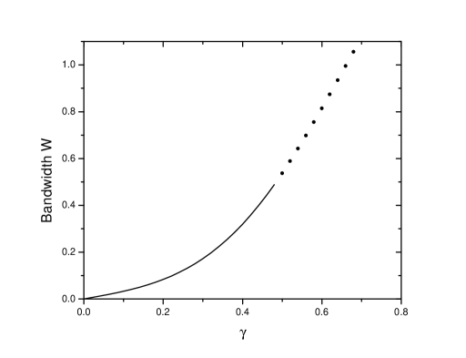
Figure 13: Bandwidth in the resonant and stronger coupling regime as a function of coupling constant $\gamma$. Here, $\Delta=\omega=t=1$. As $\gamma\gtrsim 0.6$, neighboring bands will overlap, indicated here with dotted line.

V Conclusion

We have studied the coherent dynamics of Holstein polarons in a strong electric field. We have found that with the help of phonons, a sort of quasi-continuous band will form under resonance conditions, even for weak coupling constants. The band shows approximate fractal self-similar structure, which is inherent in the near self-similarity of the Hamiltonian. Although the phonons can help the electron jump from one WS ladder state to another, the phonons can also prevent the electron from propagating, if too many phonons are involved. These peculiar interaction differences give rise to a variety of unusual states, including: (a) delocalized polarons despite the strong electric field, with a typical phonon cloud accompanying the electron; and (b) states with high degeneracy at the band center, where the electron is localized in a site of the lattice, and the phonon is located away from the electron, in a stretched configuration. The band structure is also manifested in transport properties of the system, which we expect could be observed in tunneling experiments. The level structure and extension of the different states will appear as a modulation of the phonon replicas in the tunneling experiment. For weak coupling, this would only occur if the system is in resonance, $\omega=\Delta$, as away from that condition the states are basically localized and would not transport current (except for thermal effects). In a given structure, the resonance condition can be reached by sweeping the electric field, while monitoring the tunneling through the structure. As the spacing between the deformed rungs and the localization length of the eigenfunction can be adjusted by electric field, it would be quite interesting to see the transition in experiments. With increasing coupling constant, the ‘minibands’ will overlap, and give rise to an overall merging of the phonon replicas in tunneling, even when away from the resonance regime.

- (1)
- (2) E. E. Mendez, F. Agullo-Rueda, and J. M. Hong, Phys. Rev. Lett. 60, 2426 (1988); E. E. Mendez and G. Bastard, Phys. Today 46, 34 (1993). C. Waschke, H. G. Roskos, R. Schwedler, K. Leo, and H. Kurz, Phys. Rev. Lett. 70, 3319 (1993). C. Martijin de Sterke, J. N. Bright, P. A. Krug, and T. E. Hammon, Phys. Rev. E 57, 2365 (1998); S. R. Wilkinson, C. F. Bharucha, K. W. Madison, Q. Niu, and M. G. Raizen, Phys. Rev. Lett. 76, 4512 (1996); M. B. Dahan, E. Peik, J. Reichel, Y. Castin, and C. Salomon, Phys. Rev. Lett. 76, 4508 (1996).
- (3) R. Tsu and G. H. Dohler, Phys. Rev. B 12, 680 (1975).
- (4) D. H. Dunlap and V. M. Kenkre, Phys. Rev. B. 34, 3625 (1986); Phys. Lett. A 127, 438 (1998). X.-G. Zhao, Phys. Lett. A 155, 299 (1991); 167, 291 (1992). M. Holthaus, Phys. Rev. Lett. 69, 351 (1992). W. Zhang and X.-G. Zhao, Physica E 9 , 667 (2001).
- (5) X.-G. Zhao, R. Jahnke, and Q. Niu, Phys. Lett. A 202, 297 (1995).
- (6) A. W. Ghosh, L. Jönsson, and J. W. Wilkins, Phys. Rev. Lett. 85, 1084 (2000). T. Dekorsy, A. Bartels, H. Kurz, K. Köhler, R. Hey, and K. Ploog, Phys. Rev. Lett. 85, 1080 (2000).
- (7) D. Emin and C. F. Hart, Phys. Rev. B 36, 2530 (1987).
- (8) J. Bonca and S. A. Trugman, Phys. Rev. Lett. 79, 4874 (1997).
- (9) V. V. Bryxin and Y. A. Firsov, Solid State Commun. 10, 471 (1972). V. L. Gurevich, V. B. Pevzner, and G. Iafrate, Phys. Rev. Lett. 75, 1352 (1995).
- (10) A. O. Govorov and M. V. Entin, JETP 77, 819 (1993).
- (11) A. O. Govorov, Solid State Commun. 92, 977 (1994).
- (12) L. I. Korovin and S. T. Pavlov, Sov. Phys. JETP 26, 979 (1968); S. Das Sarma and A. Madhukar, Phy. Rev. B 22, 2823 (1980); F. M. Peeters and J. T. Devreese, Phys. Rev. B, 31, 3689 (1985); 36, 4442 (1987); J.-P. Cheng, B. D. McCombe, J. M. Shi, F. M. Peeters, and J. T. Devreese, Phys. Rev. B 48, 7910 (1993).
- (13) S. V. Rakhmanova and E. M. Conwell, Appl. Phys. Lett. 75, 1518 (1999).
- (14) P. M. Petroff, A. Lorke and A. Imamoglou, Phys. Today 54, 56 (2001).
- (15) T. Holstein, Ann. Phys. (N.Y.) 8 , 343 (1959).
- (16) W. Zhang, A. O. Govorov, and S. E. Ulloa, Europhys. Lett., to appear (2002).
- (17) For references on Cayley tree properties, see for example K. Kundu and B. C. Gupta, cond-mat/9705150.
- (18) The basis described here ignores the possibility of the electron hopping against the field, while creating phonons (absorption is accounted for in this basis when jumping against the field, however). Basis states such as or , have a larger energy, produce only a small correction of the resulting states, and are ignored here. These additional basis vectors can be straightforwardly included, although greatly increasing the relevant space and associated matrices. Their inclusion is more important in the case of strong tunneling and/or coupling constant.
- (19) N. Zou, K. A. Chao, and Y. M. Galperin, Phys. Rev. Lett. 71, 1756 (1993); C. A. Stafford and N. S. Wingreen, Phys. Rev. lett. 76, 1916 (1996).
- (20) J. G. Chen, C. H. Yang, M. J. Yang, and R. A. Wilson, Phys. Rev. B 43, 4531 (1991).