Granular clustering in a hydrodynamic simulation

Abstract

We present a numerical simulation of a granular material using hydrodynamic equations. We show that, in the absence of external forces, such a system phase-separates into high density and low density regions. We show that this separation is dependent on the inelasticity of collisions, and comment on the mechanism for this clustering behavior. Our results are compatible with the granular clustering seen in experiments and molecular dynamic simulations of inelastic hard disks.

One of the key differences between a granular material and a regular fluid is that the grains of the former lose energy with each collision, while the molecules of the latter do not. Even when the inelasticity of the collisions is small, it can give rise to dramatic effects, including the Maxwell Demon effecteggers and, the topic of this paper, the phenomenon of granular clustering. Experimentskudrolli ; olafsen and molecular dynamics simulationsgoldhirsch alike show that granular gases in the absence of gravity do not become homogeneous with time, but instead form dense clusters of stationary particles surrounded by a lower density region of more energetic particles. From a particulate point of view, one can explain these clusters by noting that when a particle enters a region of slightly higher density, it has more collisions, loses more energy, and so is less able to leave that region, thus increasing the local density and making it more likely for the next particle to be captured. We, however, are interested in describing this behavior using hydrodynamics. There is considerable workkinetic deriving granular hydrodynamics from kinetic theory, focusing on analytical treatments of the long-wavelength behavior of the system. Goldhirsch and Zannettigoldhirsch , for instance, describe clustering as the result of a hydrodynamic instability: a region of slightly higher density has more collisions, and thus has a lower temperature. A lower temperature means a lower pressure, which attracts more mass from the surrounding higher-pressure region. Their long-wavelength stability analysis shows that in a system of hydrodynamic equations similar to Eq. 1, higher-density regions do indeed have lower pressure, fueling the instability. Our approach here is different. In this paper, we discuss whether a coarse-grained description, in terms of local particle, momentum, and energy densities, can be used to treat characteristic behaviors of granular materials as a self-contained dynamical system. The spirit is similar to the use of density functional theory in the treatment of freezingfreezing . We present the results of numerical simulations for such a description in the case of clustering, and show that when inelasticity is present, one indeed sees the system phase-separate into regions of high and low density.

We begin with a number density field $\rho$, a flow velocity field $\mathbf{u}$, and a “temperature”temperature field $T$. These are related by a standard set of hydrodynamic equations for granular materialshaff :

$${\partial\rho\over\partial t} = -\nabla_{i}(\rho u_{i})$$ (1)

$${\partial(\rho u_{i})\over\partial t} = -\nabla_{i}P-\nabla_{j}(\rho u_{i}u_{j})+\nabla_{j}(\eta_{ijkl}\nabla_{k}u_{l})$$ (2)

$${\partial T\over\partial t} = -\nabla_{i}(u_{i}T)+{1\over\rho}\nabla_{i}(\kappa\nabla_{i}T)$$ (4)

$$\hskip 36.135pt+\frac{1}{\rho}\eta_{ijkl}(\nabla_{i}u_{j})(\nabla_{k}u_{l})-\gamma T.$$

where repeated indices are summed over, and where $P$ is the pressure, $\kappa$ is the bare thermal conductivity, and $\eta_{ijkl}=\eta(\delta_{ik}\delta_{jl}+\delta_{il}\delta_{kj}+\delta_{ij}\delta_{kl})$ is the isotropic bare viscosity tensor. These equations bear much in common with those for normal fluidskim . The most important addition is that of the inelastic term, $-\gamma T$. The parameter $\gamma$ is a measure of the inelasticity of the collisions, and is proportional to $(1-e^{2})$, where $e$ is the coefficient of restitution. Using kinetic theory resultshaff , the transport coefficients are chosen to depend on temperature and density:

$$\kappa=\kappa_{0}T^{1/2}$$ (5)

$$\eta=\eta_{0}\rho T^{1/2}$$ (6)

$$\gamma=\gamma_{0}T^{1/2}.$$ (7)

Typically, work in granular hydrodynamics is done in low-density regimes, where grains may be treated as point particles interacting via collisions. When simulating aggregation, however, one must take excluded volume into account. We do this by introducing a barrier in the pressure $P(\rho)$ at some maximum (close-packed) density $\rho_{0}$. This is in addition to the usual hydrodynamic pressure $\rho T$. We choose in particular the simple quadratic form

$$P=\rho T+U(\rho^{2}-\rho_{0}^{2})\theta(\rho-\rho_{0}),$$ (8)

where $U$ is a positive parameter, $\theta(x)$ is the unit step function, and $\rho_{0}$ is the close-packed density. We introduced this method in an earlier paperhill , and it is a simple way to model the incompressibility of the system at high densitiesgollub .

We evaluate our equations in two dimensions using a finite-difference Runge-Kutta method, on a $100\times 100$ square lattice with periodic boundary conditions. (See footnote method for more details.) The lattice spacing is chosen to be large enough so that each site contains a number of grains, and we can consider the density to be a continuous variable. We start with random initial conditions $\rho=0.1+0.001r_{1}(z,x)$, $u_{z}=r_{2}(z,x)$, $u_{x}=r_{3}(z,x)$, and $T=1+0.1r_{4}(z,x)$, where $r_{i}(z,x)$ are random numbers chosen between $-1$ and $1$. The model’s other parameters for the data presented here are $\eta_{0}=50$, $\kappa_{0}=1$, $U=4\times 10^{4}$, $\rho_{0}=0.2$, and $\gamma_{0}=50$ or $0$. All values are in arbitrary units, with a time step of $\Delta t=10^{-3}$.

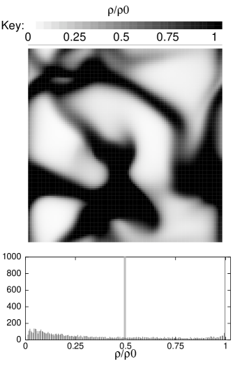
Figure 1: The density distribution at $t=800$ when $\gamma_{0}=50$, clearly showing phase separation. The top picture is a spatial distribution of the density; darker shades correspond to higher densities. The lower graph is a histogram of the density, with bin size $\Delta(\rho/\rho_{0})=0.005$. The initial distribution is shown by the light gray bar in the center.

Figure 2: The width of the density distributions, simply defined as the difference between the maximum density and the minimum density, for $\gamma_{0}=0$ and $\gamma_{0}=50$.

Figure 1 shows the density distribution for the system after it has evolved to a time $t=800$. One can clearly see that, from a narrow initial distribution centered at $\rho/\rho_{0}=0.5$, the system has separated into regions of high and low density, with relatively sharp borders. Calculating the structure factor $S(\mathbf{r})=\left\langle\delta\rho(\mathbf{r^{\prime}})\delta\rho(\mathbf{r^{\prime}}+\mathbf{r})\right\rangle_{\mathbf{r^{\prime}}}$ shows that the density is correlated out to 8 or 9 lattice spacings. To show that this clustering behavior is due to the inelastic term in Eq. 1, we duplicate the run with $\gamma_{0}=0$. Figure 2 shows the width of the density distribution as a function of time for the inelastic and elastic cases. Without inelasticity, the system quickly becomes homogeneous.

This clustering behavior of the system appears to be robust. The parameter values chosen for this run were not optimized, and a variety of alternate choices result in the same qualitative effect. The time over which clustering occurs does depend on different parameters, and in cases where the viscosity is too large, the density distribution does not form the peaks at its extremes, but instead remains broad and relatively flat. This also occurs when one removes the pressure barrier at $\rho_{0}$. In both cases, however, there is distinct and permanent phase separation.

Figure 3: Density distributions for the $\gamma_{0}=50$ case at $t=800$. The middle graph is the distribution for the entire system. The upper graph is the distribution only for those sites on the lattice where the temperature is less than $5\times 10^{-7}$. (The average temperature at this time is $1.3\times 10^{-6}$.) Similarly, the lower graph is the distribution for those sites with temperature greater than $5\times 10^{-6}$.

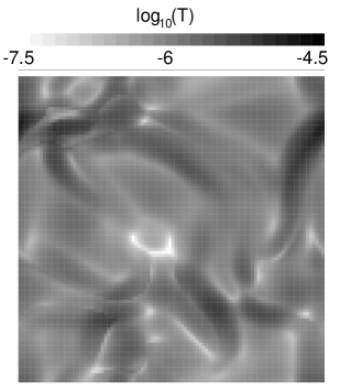
Figure 4: The spatial distribution of the log of the temperature at $t=800$. Just as before, darker shades correspond to higher temperatures. Compare this figure with Fig. 1 to look for correlations between density and temperature.

It is clear that our simulations reproduce clustering. As mentioned in the introduction, it is believed goldhirsch that clustering occurs because of an anticorrelation between density and temperature: regions of high density have more collisions, and thus more dissipation, and thus less total energy. Fig. 3 shows the density distributions corresponding to the highest and the lowest temperatures. Notice that the high-temperature distribution is missing the high-density peak present in the other two graphs. On the other hand, in the low-temperature distribution, the high-density peak is relatively larger than in the general case. Both points suggest that high-density regions tend to be at low temperatures, which agrees with the common wisdom. However, the anticorrelation is not as clear-cut as one might expect: there is no correlation between low densities and high temperatures, for instance, and even the high density sites have a broad range of temperatures which only tend toward the low side. Fig. 4 is a density plot of the temperature. When one compares this with Fig. 1, there appears to be more structure to the system than the simple explanation would suggest.

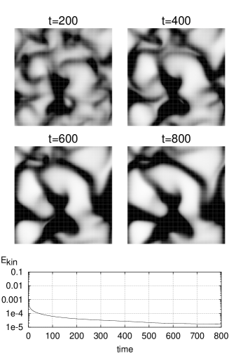
Figure 5: At the top, images of the spatial density distribution at four times, using the same key as in Fig. 1. Note that the clusters continue to move around for long periods of time. Below these, a plot showing that the average kinetic energy ($E_{kin}=\langle\rho(u_{z}^{2}+u_{x}^{2})\rangle$) is decaying at a slower-than-exponential rate.

One interesting point about the system is that it takes a long time to come to a stop. Fig. 5 shows the distribution of density at four different times. Also shown is the average kinetic energy of the system over time; it is decaying at a slower-than-exponential rate. This occurs because the viscosity, being proportional to the temperature, is decaying to zero, and is thus very small by the end of this run. It is difficult to say whether this feature corresponds to the results of experiments and other simulations, because the nature of freezing in gravity-free granular systems is generally subtle. In event-driven molecular dynamic simulations, one finds the phenomenon of inelastic collapseinelastic , where particles on the verge of freezing in a cluster suffer an infinite number of collisions in a finite amount of time. In experimentolafsen , there is the opposite effect: one must vibrate real two-dimensional systems of particles to create clustering, as the surface friction will otherwise freeze the system before any clustering can occur. If desired, one could bring our model to a halt with the introduction of a surface friction term, or by replacing the current temperature dependence of the viscosity with

$$\eta\propto\eta_{0}\rho(T+T_{\min})^{1/2}.$$ (9)

In summary, we have recreated in hydrodynamic simulation the clustering behavior in granular materials which was predicted by hydrodynamic theory and observed in kinetic simulations. We show that this behavior is directly dependent on the inelasticity parameter of our equations. This supports the notion that granular materials can be, to some extent at least, described by means of coarse-grained variables in a nonlinear hydrodynamical setting. However, we also suggest that long-wavelength hydrodynamics alone may not be sufficient to fully describe granular behavior, such as the actual mechanism for granular clustering.

We thank Professor Todd DuPont for his assistance in constructing our simulations, and Professors Heinrich Jaeger, Sidney Nagel, and Thomas Witten for helpful conversations. This work was supported by the Materials Research Science and Engineering Center through Grant No. NSF DMR 9808595.

References

- (1) J. Eggers, Phys. Rev. Lett. 83, 5322 (1999).
- (2) A. Kudrolli, M. Wolpert, and J.P. Gollub, Phys. Rev. Lett. 78, 1383 (1997).
- (3) J.S. Olafsen and J.S. Urbach, Phys. Rev. Lett. 81, 4369 (1998).
- (4) I. Goldhirsch and G. Zanetti, Phys. Rev. Lett. 70, 1619 (1993).
- (5) P.K. Haff, J. Fluid Mech. 134, 401 (1983); and J.T. Jenkins and S.B. Savage, J. Fluid Mech. 130, 187 (1983). More recently, J.J. Brey, M.J. Ruiz-Montero, and D. Cubero, Phys. Rev. E 60, 3150 (1999); T.P.C. van Noije and M.H. Ernst, Gran. Matt. 1, 57 (1998); J.J. Brey, J.W. Dufty, C.S. Kim, and A. Santos, Phys. Rev. E 58, 4638 (1998).
- (6) T.V. Ramakrishnan and M. Yussouff, Phys. Rev. B 19, 2775 (1979).
- (7) The temperature here is not thermal, but actually a measure of the local energy density that is not accounted for by the local flow velocity: . Apart from this equation, it is not necessary to assume that this quantity has any properties normally associated with temperature.
- (8) P.K. Haff, J. Fluid Mech. 134, 401 (1983).
- (9) B. Kim and G.F. Mazenko, J. Stat. Phys. 64, 631 (1991). See also hill .
- (10) S.A. Hill and G.F. Mazenko, Phys. Rev. E 63, 031303 (2001). The actual structure of the free energy density (to which pressure is related by ) in our previous paper is more complex than what we use here, but it does possess the high-density barrier to account for the ultimate incompressibility of the grains.
- (11) Others have dealt with the high-density limit by having the viscosity diverge as the density approaches its maximum value. See, for example, W. Losert et al., Phys. Rev. Lett. 85, 1428 (2000).
- (12) Some details about our methods: (1) Our Runge-Kutta method includes an adaptive time step; it, however, is rarely activated since we use a default time step that is suitably small. (2) We offset the velocities from the other fields on the lattice such that the densities and temperatures may be considered to lie on the faces of the lattice while the horizontal (vertical) velocities lie on the vertical (horizontal) edges. (3) We have had great numerical difficulty with regions of very low density: such regions have a tendency to drift below zero density or generate large velocities in an unnatural fashion. We use an upwind technique to evaluate the equation , to prevent the density from becoming negative. In addition, we prevent mass from flowing out of any site with a density below some minimum value ().
- (13) B. Bernu and R. Mazighi, J. Phys. A 23, 5745 (1990); S. McNamara and W.R. Young, Phys. Fluids A 4, 496 (1992); T. Zhou and L.P. Kadanoff, Phys. Rev. E 54, 623 (1996).