Effective electron-electron interaction in a two dimensional paramagnetic system

Abstract

We analyze the effective electron-electron interaction in a two dimensional polarized paramagnetic system. The spin degree of freedom, s, is manifestly present in the expressions of spin dependent local field factors that describe the short range exchange (x) and correlation (c) effects. Starting from the exact asymptotic values of the local field correction functions for large and small momentum at zero frequency we obtain self-consistent expressions across the whole spectrum of momenta. Then, the effective interaction between two electrons with spins s and s’ is calculated. We find that the four effective interactions, up-up, up-down, down-up and down-down, are different. We also obtain their qualitative dependence on the electronic density and polarization and note that these results are independent of the approximation used for the local field correction functions at intermediate momenta.

I Introduction

To accomplish spin dependent conduction in electronic devices has become a very intense quest in recent years. review The II-VI dilute magnetic semiconductors, like CdMnTe and ZnMnSe, seem to be the most promising materials for achieving this goal. At low doping levels these systems exhibit an enhanced Zeeman splitting of the electronic levels that arises from strong Kondo-like exchange between the embedded Mn ions and the delocalized electronic states. Moreover, the II-VI dilute magnetic semiconductors are n-type conductors with relative good mobility and large spin coherence times ($\sim 10ns$). However, an open question remains as to how the magnetic interaction between the localized spins and the itinerant carriers reflects on the transport properties of these structures. The purpose of this work is to analyze some aspects of this problem.

Since the Zeeman splitting of the electron levels was found to be independent of the local magnetic environment crooker95 , a simple model of a II-VI magnetic semiconductor is a spin polarized electron gas in the presence of a static magnetic field. The field lifts the spin degeneracy and induces an equilibrium polarization, $\zeta=(n_{\uparrow}-n_{\downarrow})/(n_{\uparrow}+n_{\downarrow})$. The strong magnetic interaction between the itinerant carriers and the localized spins is reflected in the large value of the effective gyromagnetic factor, $\gamma^{*}$, up to hundreds of times the band value. On account of the large $\gamma^{*}$, even low magnetic fields are enough to produce large polarizations, and it is assumed that $\zeta$ can vary continuously between $-1$ and $1$ as a function of the static magnetic field. This approximation integrates out the degrees of freedom of the static spins under the enlarged value of $\gamma^{*}$ and focuses on the itinerant carriers and the many body interaction among them. The latter is independent of the source of the spin polarization, and we expect our results to maintain their validity also in the case of a self-consistent magnetic field as source of the spin polarization, a situation which is consistent with an itinerant ferromagnet. The model can also be extended to describe the paramagnetic state of the III-V magnetic heterostructures where a mostly uniform internal magnetic field is created by having a magnetic ion density much larger than the itinerant-carrier density. mune89 ; ohno92 However, the small electronic densities in the III-V based compounds make difficult the blind use of the paramagnetic electron gas model.

The explicit spin dependence of the electron-electron interaction becomes manifest when the exchange (x) and correlation (c) effects of the local Coulomb repulsion are included. At finite values of the polarization, the many-body short range interaction, which is density dependent, is different for up and down spin electrons. A realistic picture of the electronic interaction and its screening is obtained by using spin dependent local field correction functions, $G^{x,c}_{\sigma}({\bf q},\omega)$, that describe the exchange and correlation hole around each electron. The self consistent treatment of exchange and correlation effects has proved very important in understanding the physics of normal metals, mahan but to our knowledge it has not been fully analyzed in spin-polarized systems, where the spin dependence of the local field corrections becomes manifest. In addition, the relevance of exchange and correlation effects increases as the dimensionality of the electron gas is lowered. For example, the importance of local effects is clearly reflected in the dielectric function of an unpolarized two-dimensional electron gas, which becomes overscreened in a wide range of momenta and electronic density. pede97 However, calculations where these effects are absent, such as the conventional random phase approximation, predict a positive dielectric function for the whole parameter range. Therefore, we believe it is fundamental to include these local effects in a complete treatment of the quasi-two-dimensional diluted magnetic semiconductors.

Obtaining the exact frequency and wave vector dependence of the local field corrections is a very difficult problem which remains unsolved even in the case of the unpolarized electron system. Fortunately, the asymptotic values of the local field factors can be obtained exactly in two limiting cases. At zero frequency and small wavevectors, sum rules are used to connect the static limits of the response functions to certain thermodynamic coefficients. mar02 For large frequency and large wavevector, an iterative method generates the exact expressions for the local field functions up to second order. niklasson This approach uses the equation of motion satisfied by the Wigner distribution function of the particle density.

Numerical estimates of the response functions of the three dimensional unpolarized electron gas have shown that local field factors smoothly interpolate between the asymptotic small and large wave-vector behavior.Moro95 This feature is expected to exist also in the case of a spin polarized system, and, consequently, we use the exact asymptotic values of $G^{x,c}_{\sigma}({\bf q},\omega)$ for large and small momentum at zero frequency mar02 ; mar97 ; pol01 as a starting point in obtaining their approximate expressions across the whole spectrum of momentum. Then, $G_{\sigma}({\bf q},\omega)$ are used to calculate the spin dependent effective electron interaction potentials, ${{\cal V}_{\sigma\sigma^{\prime}}}({\bf q},\omega)$. We compare two interpolation schemes to conclude that the effective potentials are qualitatively independent of the approximation used for the local field correction functions at intermediate momenta.

In section II, we present the self consistent formulation of the effective interaction that incorporates the spin dependent local field corrections following the approach of Kukkonen and Overhauser kuk79 ; zhu86 generalized for a spin polarized electron system.yi96 This formalism permits the derivation of the effective spin dependent scattering potentials experienced by an electron and of the response functions. In section III, we discuss in detail the procedure used to obtain the approximate expressions for the local field factors. Section IV presents our conclusions. The appendix is dedicated to a derivation of the correlation function of a two dimensional electron gas at the origin.

II Effective interaction potentials

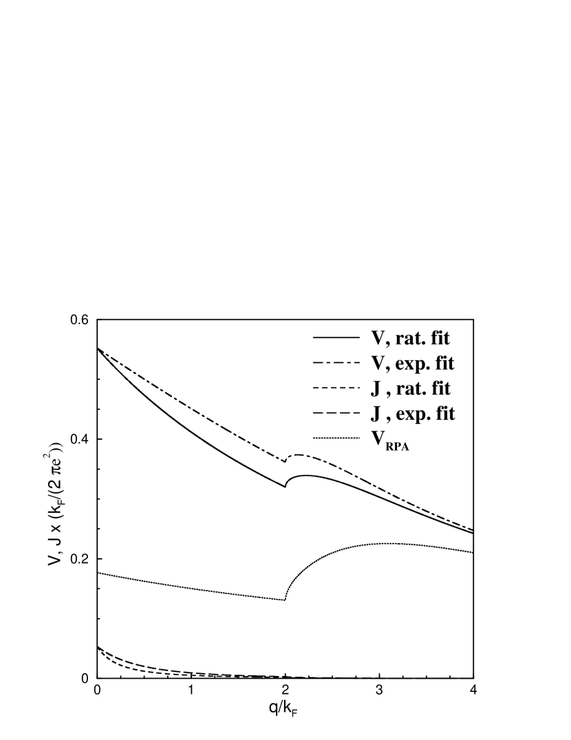
Figure 1: Normalized static effective interactions $V({\bf q},\omega=0)$ and $J({\bf q},\omega=0)$ for an unpolarized electron gas ($\zeta=0$) as functions of the normalized momentum ${\bf q}/k_{F}$ for $r_{s}=4$. Results using a rational (Eq. (11)) and an exponential (Eq. (12)) fit for the local field correction functions are displayed. Note the similarity of the results for the two fittings. Results for the random phase approximation are also displayed.

Figure 2: Normalized static effective interactions $V_{\sigma}({\bf q},\omega=0)$ and $J_{\sigma}({\bf q},\omega=0)$ for a polarization of $\zeta=0.5$ as functions of the normalized momentum ${\bf q}/k_{F}$ for $r_{s}=4$. Results for the random phase approximation are also displayed. We have used a rational fit (Eq. (11)) for the local field corrections.

Figure 3: Normalized effective interaction $V_{eff}({\bf q})$ for an unpolarized electron gas ($\zeta=0$) as a function of the normalized momentum ${\bf q}/k_{F}$ for $r_{s}=4$. Results using a rational (Eq. (11)) and an exponential (Eq. (12)) fit for the local field correction functions as well as results for the random phase approximation are displayed. Note that the RPA interaction is the same as that in Fig. 1.

Figure 4: Normalized effective interaction $V_{eff}({\bf q})$ for a polarization of $\zeta=0.5$ as a function of the normalized momentum ${\bf q}/k_{F}$ for $r_{s}=4$. Results using a rational (Eq. (11)) and an exponential (Eq. (12)) fit for the local field correction functions as well as results for the random phase approximation are displayed. The RPA curve is the same as that in Fig. 2.

The simplest approximation of the effective interaction in the electron gas is the random phase approximation (RPA), which incorporates the screening but ignores the exchange and correlation effects. Therefore, all spin dependence is lost. A more realistic description, which considers the short range Coulomb interaction effects, was proposed by Hubbard, Hubb57 whose expression for the dielectric constant introduces the local field correction, a wavevector dependent function that describes the difference between the real particle density and its mean field (RPA) counterpart.

The microscopic origin of the local field corrections was elucidated by Kukkonen and Overhauser. kuk79 In their model of the electron-electron interaction, the exchange (x) and correlation (c) are explicitly incorporated by considering associated local field factors, $G(\bf{q},\omega)$, in the expression of the effective potential experienced by one electron in the presence of all the rest. In a self-consistent formulation, the details of which will be given below in the case of a spin polarized electron system, this theory leads to the Hubbard dielectric function. The method is equivalent to considering the many body interaction in all orders, as it has been shown by using diagrammatic techniques. Vig85

In the case of a spin polarized system, it is appropriate to introduce spin dependent local field corrections because the many body effects are density dependent, and they depend on the spin directly through the exclusion principle.yi96 In a direct generalization of Ref. kuk79, , the effective potential $\widetilde{\cal V}_{\sigma\sigma^{\prime}}$ experienced by an electron with spin $\sigma$ in the presence of an second electron with spin $\sigma^{\prime}$ and charge density $\rho({\bf q})$ can be written as: spin-flip

$$\widetilde{\cal V}_{\sigma\sigma^{\prime}}({\bf q},\omega)=v({\bf q})\Big{\{}[1-G^{+}_{\sigma}({\bf q},\omega)](\rho({\bf q})+\Delta n({\bf q},\omega))$$

$$-\sigma G^{-}_{\sigma}({\bf q},\omega)(\sigma^{\prime}\rho({\bf q})+\Delta m_{z}({\bf q},\omega))\Big{\}}$$ (1)

where $\Delta n=\Delta n_{\uparrow}+\Delta n_{\downarrow}$ and $\Delta m_{z}=\Delta n_{\uparrow}-\Delta n_{\downarrow}$ are the particle and spin density fluctuations, respectively, induced by the presence of the second electron, and $v(q)$ is the bare Coulomb interaction, which is equal to $2\pi e^{2}/q$ in two dimensions. The local field functions $G^{\pm}_{\sigma}({\bf q},\omega)$ incorporate the exchange ($G^{x}_{\sigma}$) and correlation effects ($G^{c}_{\sigma\sigma},G^{c}_{\sigma\bar{\sigma}}$), which induce a local decrease in the electronic density around an electron of given spin $\sigma$ compared with its RPA value.  $G^{+}_{\sigma}({\bf q},\omega)$ is the sum of all same and opposite spin effects, and $G^{-}_{\sigma}({\bf q},\omega)$ is the difference of same and opposite spin effects: $G^{\pm}_{\sigma}({\bf q},\omega)=G^{x}_{\sigma}+G^{c}_{\sigma\sigma}\pm G^{c}_{\sigma\bar{\sigma}}$. same-spin In brief, Eq. (II) shows how the electron charge density is decreased from the corresponding RPA value to account for its own short range effects.

The role played by $G^{+}_{\sigma}$ and $G^{-}_{\sigma}$ in the physical properties of the electron gas is quite different. For an unpolarized electron gas, $G^{+}$ enters the electrical response functions, and $G^{-}$ the magnetic response. It is well known that in this limit the dielectric function and the electronic susceptibility can be written down as functions of $G^{+}({\bf q})$ and $G^{-}({\bf q})$ respectively: kuk79

$$\epsilon({\bf q},\omega)=1-\frac{v_{q}\Pi({\bf q},\omega)}{1+G^{+}({\bf q})v_{q}\Pi({\bf q},\omega)}$$ (2)

$$\chi({\bf q},\omega)=\frac{-\gamma^{*2}\Pi({\bf q},\omega)}{1+G^{-}({\bf q})v_{q}\Pi({\bf q},\omega)}$$ (3)

where $\gamma^{*}$ is the enhanced effective gyromagnetic ratio and $\Pi=\Pi_{\uparrow\uparrow}+\Pi_{\downarrow\downarrow}$ is the polarization function. However, in a polarized gas both local field factors are interconnected and appear in the expressions of the dielectric function and the magnetic susceptibility.

In a linear approximation, the density fluctuations are proportional to the effective potentials, where the proportionality coefficients are appropriately defined polarization functions: $\Delta n_{\uparrow}=\Pi_{\uparrow\uparrow}\widetilde{\cal V}_{\uparrow,\sigma^{\prime}}$ ($\Delta n_{\downarrow}=\Pi_{\downarrow\downarrow}\widetilde{\cal V}_{\downarrow,\sigma^{\prime}}$). Here $\Pi_{\sigma\sigma^{\prime}}$ is the generalized polarization bubble for the non-interacting electron gas,

$$\Pi_{\sigma\sigma^{\prime}}({\bf q},\omega)=\frac{1}{V}\sum_{\bf k}\frac{n_{\bf k,\sigma}-n_{\bf k+\bf q,\sigma^{\prime}}}{\omega+\xi_{\bf k\sigma}-\xi_{\bf k+\bf q\sigma^{\prime}}}$$ (4)

where $\xi_{\bf k\sigma}=\epsilon_{\bf k}+\mbox{sign}(\sigma)\gamma^{*}B$ is the single particle energy in the static magnetic field B, $n_{\bf k,\sigma}$ is the occupation function, and V is the volume of the system. Eq. (4) generates the well known expressions for the polarization function of the non-interacting electron gas when the usual simplifications are considered: zero temperature and a parabolic energy dispersion, $\epsilon_{\bf k}=\hbar^{2}k^{2}/2m^{*}$, where $m^{*}$ is the electronic band mass. Neither approximation is expected to modify our results.

Therefore, in two dimensions the polarization operator for the complex frequency $i\omega$ is: Stern67

$$\Pi_{\sigma\sigma}(\tilde{q},i\widetilde{\omega})=\frac{k^{2}_{F}}{E_{F}}\Big{(}-\frac{1}{4\pi}\Big{)}\Big{\{}1-\frac{\widetilde{k}_{F\sigma}}{\tilde{q}}$$

$$\Big{[}(i\widetilde{\omega}+\tilde{q}^{2})\sqrt{\Big{(}\frac{1}{2\tilde{q}\widetilde{k}_{F\sigma}}\Big{)}^{2}-\Big{(}\frac{1}{i\widetilde{\omega}+\tilde{q}^{2}}\Big{)}^{2}}+c.c\Big{]}\Big{\}}$$ (5)

where $\tilde{q}=q/k_{F}$ is the normalized momentum, $\widetilde{k}_{F\sigma}=k_{F\sigma}/k_{F}$ the normalized Fermi momenta of the spin $\sigma$ electronic population, and $\widetilde{\omega}=\omega/E_{F}$ the normalized frequency. The use of normalized variables allows us to express easily all our results in terms of our only free parameter: the effective electronic density, or the ratio between $r_{s}$ and the effective Bohr radius of the system, $a^{*}_{B}=\hbar^{2}/(m^{*}e^{*2})$.numbers The retarded polarizability can be obtained by analytical continuation.

The truly effective interaction potentials, which are used in the calculation of scattering amplitudes, are obtained from $\widetilde{\cal V}_{\sigma\sigma^{\prime}}$ by subtracting the direct exchange and correlation between the two electrons: the term $v(q)\rho({\bf q})[-G^{+}_{\sigma}({\bf q})-\sigma\sigma^{\prime}G^{-}_{\sigma}({\bf q})]$ in Eq. II. Thus, the effective interaction can be expressed as:

$${\cal V}_{\sigma,\sigma^{\prime}}=V_{\sigma^{\prime}}-J_{\sigma^{\prime}}\sigma\cdot\sigma^{\prime}$$ (6)

where the first term includes the bare Coulomb interaction and the interaction mediated by charge fluctuations, and the second term reflects the interaction mediated by spin fluctuations. In an unpolarized electron gas, $V$ and $J$ are spin independent. In addition, $V$ depends only on $G^{+}$ while $J$ depends only on $G^{-}$, as it was shown in Ref. kuk79, . However, the imbalance between the two spin populations in a spin polarized electron gas induces a dependence on the spin index. Thus, $V_{\sigma}$ and $J_{\sigma}$ are:

$$V_{\sigma} = [{v_{\bf q}\rho_{\bf q}}/{D({\bf q},\omega)}]\Big{\{}1+\frac{1}{2}[G^{+}_{\sigma}+G^{+}_{\bar{\sigma}}+G^{-}_{\sigma}-G^{-}_{\bar{\sigma}}][D({\bf q},\omega)-1]+v_{\bf q}\Pi_{{\bar{\sigma}}{\bar{\sigma}}}[G^{-}_{\sigma}(1-G^{+}_{\bar{\sigma}})+G^{-}_{\bar{\sigma}}(1-G^{+}_{\sigma})]\Big{\}}$$ (7)

$$J_{\sigma} = -[{v_{\bf q}\rho_{\bf q}}/{D({\bf q},\omega)}]\Big{\{}\frac{1}{2}[G^{+}_{\sigma}-G^{+}_{\bar{\sigma}}+G^{-}_{\sigma}+G^{-}_{\bar{\sigma}}][D({\bf q},\omega)-1]+v_{\bf q}\Pi_{\bar{\sigma}\bar{\sigma}}[G^{-}_{\sigma}(1-G^{+}_{\bar{\sigma}})+G^{-}_{\bar{\sigma}}(1-G^{+}_{\sigma})]\Big{\}}$$ (8)

where     $D({\bf q},\omega)=[1-v_{\bf q}(1-G^{+}_{\uparrow}-G^{-}_{\uparrow})\Pi_{\uparrow\uparrow}][1-v_{\bf q}(1-G^{+}_{\downarrow}-G^{-}_{\downarrow})\Pi_{\downarrow\downarrow}]-[1-G^{+}_{\uparrow}+G^{-}_{\uparrow}][1-G^{+}_{\downarrow}+G^{-}_{\downarrow}]v^{2}_{\bf q}\Pi_{\uparrow\uparrow}\Pi_{\downarrow\downarrow}$.

Figs. 1 and 2 show the static effective interactions $V_{\sigma}({\bf q},\omega=0)$ and $J_{\sigma}({\bf q},\omega=0)$ between point-like electrons Fourier in a two dimensional electron gas as functions of the normalized momentum $q/k_{F}$. Fig. 1 displays the results for an unpolarized electron gas. Fig. 2 corresponds to a $\zeta=0.5$ polarization. We have chosen $r_{s}=4$, where $r_{s}$ is measured in units of the effective Bohr radius of the system. numbers The expressions used for the local field corrections are discussed in the following section. For comparison, we also include the RPA effective interaction potential, $V_{RPA}({\bf q},\omega=0)$, obtained from equation (7) by neglecting the local field corrections. Note that $J_{RPA}({\bf q},\omega=0)=0$, since the interaction mediated by spin fluctuations is directly proportional to the local corrections.

Fig. 1 shows clearly the importance of the local effect in the calculation of physical properties. First, as we have already mentioned, the spin mediated interaction, $J_{\sigma}({\bf q},\omega)$, becomes noticeable. Second, $V_{\sigma}({\bf q},\omega)$ is greatly enhanced at small momenta in comparison with the RPA prediction. In addition, Fig. 2 shows how both effective interactions split when the electron gas is polarized, an effect also absent in the RPA approach. The splitting of $J_{\sigma}({\bf q},\omega)$ is more pronounced that the splitting of $V_{\sigma}({\bf q},\omega)$ and, even, $J_{\downarrow}$ becomes negative for intermediate momenta.

Larger values of the polarization induce larger splitting of the up and down effective interactions until a spin wave instability is reached. For the density value we are considering ($r_{s}=4$), this instability happens at $\zeta\sim 0.72$. At that value of the polarization, $J_{\sigma}({\bf q},\omega)$ and $V_{\sigma}({\bf q},\omega)$ diverge for a certain value of the momenta that define the periodicity of the spin density wave.

In order to have a complete picture of the effective interactions, we also discuss the effective interaction which is used to calculate the electronic selfenergy. It can be derived in a similar manner using the self-consistent relation established between the density fluctuations and the effective potential induces by an external charge. Mor02 This effective interaction can be written as $\displaystyle V_{eff}=\frac{v({\bf q})}{\epsilon({\bf q},\omega=0)}$, where $\epsilon({\bf q},\omega)$ is the dielectric function of a polarized electron gas:

$$\epsilon({\bf q},\omega)=1-v_{{\bf q}}\frac{\Pi_{\uparrow\uparrow}+\Pi_{\downarrow\downarrow}+2v_{\bf q}(G^{-}_{\uparrow}+G^{-}_{\downarrow})\Pi_{\uparrow\uparrow}\Pi_{\downarrow\downarrow}}{\widetilde{D}({\bf q},\omega)}$$ (9)

where     $\widetilde{D}({\bf q},\omega)=[1+v_{\bf q}(G^{+}_{\uparrow}+G^{-}_{\uparrow})\Pi_{\uparrow\uparrow}][1+v_{\bf q}(G^{+}_{\downarrow}+G^{-}_{\downarrow})\Pi_{\downarrow\downarrow}]-[G^{+}_{\uparrow}-G^{-}_{\uparrow}][G^{+}_{\downarrow}-G^{-}_{\downarrow}]v^{2}_{\bf q}\Pi_{\uparrow\uparrow}\Pi_{\downarrow\downarrow}$.

Fig. 3 displays $V_{eff}({\bf q})$ for an unpolarized electron gas with the same density as before ($r_{s}=4$). Since $V_{eff}({\bf q})$ represents the electrostatic potential seen by a spinless test charge,kuk79 it is very illustrative to compare it with the RPA result, $\displaystyle V_{RPA}=\frac{v({\bf q})}{\epsilon_{RPA}({\bf q},\omega=0)}$. RPA We find that by including the local factors the effective interaction becomes overscreened for ${\bf q}$ less than a critical value, ${\bf q}_{c}$, which depends on the electronic density and the polarization. Similar results for zero polarization were reported previously. bul96 The critical value of the momentum ${\bf q}_{c}$ depends weakly on the approximation used for the local field factors. Therefore, the effective interaction with local field corrections is very different from the RPA effective interaction which is always positive. Fig. 4 displays $V_{eff}({\bf q})$ for an electron gas with $\zeta=0.5$. The overscreened region is also present, and the singularities at the Fermi momenta of the majority and minority spin populations are clearly seen.

III Spin Dependent Local Field Corrections

Figure 5: Initial slope of the local field correction function $\alpha^{+}_{\uparrow}$ as a function of the polarization ($\zeta$) for different values of $r_{s}$ as indicated in the legend.

Figure 6: Initial slope of the local field correction function $\alpha^{-}_{\uparrow}$ as a function of the polarization ($\zeta$) for different values of $r_{s}$.

Any quantitative calculation of the effects of the electron-electron interaction on many physical properties of interest requires the knowledge of the correct form of the local field correction functions. As we have already mentioned, obtaining the exact frequency and wave vector dependence of these functions has been an elusive problem. Our first approximation is to neglect the frequency dependence of the local field corrections. Although the local field functions represent a dynamical effect, they vary slowly on the scale of the Fermi frequency, hol79 ; pede97 and it is acceptable to neglect their frequency dependence.

The exact asymptotic values of $G^{\pm}_{\sigma}({\bf q},\omega)$ for large pol01 and small momentummar02 at zero frequency have been obtained previously and are summarized in Table 1, where $\tilde{q}=q/k_{F}$ and $g(0)$ is the two-particle correlation function at the origin. Note that the values of $G^{x,\pm}_{\sigma}({\bf q}=0)$ included in the table have been derived by considering only the contribution coming from the electronic exchange energy. The proper expression for $G^{\pm}_{\sigma}({\bf q}=0)$ incorporates also a combination of derivatives of the correlation energy of the system,mar02 that need to be added to the values given in Table 1.

If only the exchange contribution is considered, $G^{+}({\bf q}=0)=G^{-}({\bf q}=0)$ for the unpolarized electron gas. Using the asymptotic values from Table 1 and the previously obtained expressions for the dielectric function [Eq. (2)] and magnetic susceptibility [Eq. (3)], we find that in the static limit both response functions develop a pole for $r_{s}\geq\pi/\sqrt{2}\sim 2.221$. Note that a pole in the dielectric function does not indicate an instability of the paramagnetic phase, it just implies the appearance of a region in momentum space where the Coulomb interaction is overscreened. Dolgov81 However, a pole in the susceptibility points towards a spin density wave instability. Since numerical calculations have shown the stability of the paramagnetic phase for $r_{s}\lesssim 30$Tan89 it is crucial to include the correlation energy in the calculation of the local field factors. Including the correlations in $G^{\pm}_{\sigma}$ prevents the occurrence of a spin/charge density wave instability in the two-dimensional unpolarized electron gas.

Even though there are numerous calculations of the correlation energy of an unpolarized electron gas, approximate expressions for the correlation energy of a polarized electron gas are less numerous due to the fact that the magnetic response functions are computationally harder to obtain. MCsusc For the two dimensional electron gas we use the Monte Carlo calculation by Tanatar and Ceperley, Tan89 where the correlation energy is expressed in the form of an analytic interpolation formula: $E_{c}(r_{s},\zeta)=E_{c}(r_{s},\zeta=0)+\zeta^{2}(E_{c}(r_{s},\zeta=1)-E_{c}(r_{s},\zeta=0))$, where $E_{c}(r_{s},\zeta=0)$ and $E_{c}(r_{s},\zeta=1)$ are approximated using a Padé scheme.

By including the contribution from the correlation energy, we derived analytical expressions for the initial slope of the local field correction functions $\alpha^{\pm}_{\sigma}=G^{\pm}_{\sigma}(\tilde{\bf q}\rightarrow 0)/(\tilde{\bf q})^{d-1}$, where $d$ is the dimension of the system. These initial slopes are function of the density and the polarization of the electron gas. The behavior of $\alpha^{+}$ and $\alpha^{-}$ is quite different. Fig. 5 shows $\alpha^{+}_{\uparrow}$ for a two dimensional gas as function of the polarization for several values of $r_{s}$. Note that $\alpha^{+}_{\uparrow}$ is always positive, as it should be, since local effects always decrease the bare electron charge density. On the other hand, $\alpha^{-}_{\uparrow}$ depends strongly on the polarization for any electronic density as it can be seen in Fig. 6 where $\alpha^{-}_{\uparrow}$ is displayed. In our approximation $\alpha^{-}_{\uparrow}$ diverges for a fully polarized electron gas and, as a consequence, $G^{-}_{\uparrow}({\bf q})$ becomes a constant and equal to its value at ${\bf q}\rightarrow\infty$. In addition, $\alpha^{-}_{\uparrow}$ becomes negative in diluted systems and small polarizations. negalpha This behavior favors the stability of the paramagnetic phase. Note that similar arguments apply to $\alpha^{\pm}_{\downarrow}$ due to the fact that $\alpha^{\pm}_{\downarrow}(\zeta)=\alpha^{\pm}_{\uparrow}(-\zeta)$.

Table 1: Exact asymptotic values of the local-field factors $G^{\pm}_{\sigma}({\bf q},\omega=0)$ of a two dimensional electron gas for large and small ${\bf q}$ at zero frequency. $G^{\pm}_{\sigma}({\bf q}\rightarrow\infty)$ was calculated in Ref. pol01, . The values of $G^{x,\pm}_{\sigma}({\bf q}=0)$ are derived from Ref. mar02, considering only the contribution coming from the electronic exchange energy.

$G^{+}_{\uparrow}({\bf q}\rightarrow\infty)$	$1-(1-\zeta)g(0)$
$G^{-}_{\uparrow}({\bf q}\rightarrow\infty)$	$(1-\zeta)g(0)$
$G^{x,+}_{\uparrow}({\bf q}\rightarrow 0)$	$(\tilde{q}/(2\pi))\big{\{}\zeta\sqrt{1+\zeta}+(2-\zeta)\sqrt{1-\zeta}\big{\}}$
$G^{-}_{\uparrow}({\bf q}\rightarrow 0)$	$(\tilde{q}/(2\pi))\big{\{}[(2+\zeta)/\sqrt{1+\zeta}]+[\zeta/\sqrt{1-\zeta}]\big{\}}$

Figure 7: Local field corrections $G^{\pm}_{\sigma}({\bf q},\omega=0)$ versus normalized momentum ${\bf q}/k_{F}$ for a two dimensional unpolarized electron gas with $r_{s}=4$. Results for the rational fit (Eq.( 11)) (solid curves) and for the exponential fit (Eq. ( 12)) (dashed curves) are displayed. The inset is a blow-up of the lower corner with the $G^{-}$ functions.

Figure 8: Local field corrections $G^{\pm}_{\sigma}({\bf q},\omega=0)$ versus normalized momentum ${\bf q}/k_{F}$ for a two dimensional electron gas with $r_{s}=4$ and polarization $\zeta=0.5$. Results for the rational fit (Eq.( 11)), $G^{\pm}_{\uparrow}$ (dotted curves) and $G^{\pm}_{\downarrow}$ (solid curves) and for the exponential fit (Eq. ( 12)), $G^{\pm}_{\uparrow}$ (dashed) and $G^{\pm}_{\downarrow}$ (long-dashed) are displayed. The inset is also a blow-up of the lower corner with the $G^{-}$ functions.

General expressions for $G^{\pm}_{\sigma}({\bf q})$ can be interpolated between the large and small momentum limits. The simplest way to interpolate $G^{+}({\bf q})$ for a regular metal was first suggested by Hubbard: Hubb57

$$G^{+}({\bf q})=\frac{\alpha{\bf q}^{2}}{1+\Big{(}\alpha/G^{+}(\infty)\Big{)}{\bf q}^{2}}$$ (10)

In a later work, Singwi and collaborators sing70 ; vash72 remarked that their numerical results for $G^{+}({\bf q})$ in an unpolarized three dimensional gas could be adequately fitted by the simpler expression $G^{+}({\bf q})=A\Big{(}1-e^{-B{\bf q}^{2}}\Big{)}$, where the two fitting parameters are smoothly varying functions of the electronic density. They noted that this expression fits their results well at small and intermediate values of momentum but not at larger values. However, $G^{+}({\bf q})$ is relatively unimportant at large q. Similar conclusions have been reached for the unpolarized two dimensional electron gas, bul96 where the argument of the exponential is linear rather than quadratic. However, the possibility that $G^{+}({\bf q})$ have a peak near $q=2k_{F}$, Wang84 as a residue of the sharp peak in the exchange potential, is a long standing issue. Recent calculations show that the inclusion of short-range correlations has the effect of washing out this peak. pede97

Approximate expressions for $G^{-}({\bf q})$ are less numerous, partly due to the fact that $G^{-}$ is related to the magnetic response functions, which are computationally challenging. MCsusc In addition, it is known that for a three dimensional gas, $G^{-}({\bf q})$ can not be a monotonic function of momentum because its slope at ${\bf q}=0$ is positive but asymptotically approaches a negative value at large momentum. Zhu and Overhauser zhu86 suggested a simple rational function with a maximum at ${\bf q}=2k_{F}$.

Our approach shows that the initial slope of the local field correction functions $G^{+}_{\sigma}({\bf q})$ is always positive. In contrast, the initial slope of $G^{-}_{\sigma}({\bf q})$ could be negative for diluted systems and small values of the polarization. In the large momentum limit, $G^{\pm}_{\sigma}({\bf q}\rightarrow\infty)$ is always positive in two dimensions. However, in three dimensions $G^{+}_{\uparrow}({\bf q}\rightarrow\infty)$ might be negative for $\zeta\leq-2/3$, and $G^{-}_{\uparrow}({\bf q}\rightarrow\infty)$ is negative for all values of the polarization if the electron density verifies $r_{s}\geq 1.18$. largeq

Given the diversity of behaviors in the limiting values of the local field correction functions, we consider a general interpolating scheme for all the cases. For a value of the polarization $\zeta$ and of the electron density $r_{s}$, we calculate the product $\alpha^{\pm}_{\sigma}G^{\pm}_{\sigma}(\tilde{\bf q}\rightarrow\infty)$ where $\alpha^{\pm}_{\sigma}$ has been defined previously. When $\alpha^{\pm}_{\sigma}G^{\pm}_{\sigma}(\tilde{\bf q}\rightarrow\infty)>0$, we use the following fitting expressions for the local field factors:

$$G^{\pm}_{\sigma}(\tilde{\bf q})=\frac{\alpha^{\pm}_{\sigma}\tilde{\bf q}^{d-1}}{1+\Big{(}\alpha^{\pm}_{\sigma}/G^{\pm}_{\sigma}(\infty)\Big{)}\tilde{\bf q}^{d-1}},\hskip 14.22636pt{\rm rational\hskip 5.69046ptfit};$$ (11)

$$G^{\pm}_{\sigma}(\tilde{\bf q})=G^{\pm}_{\sigma}(\infty)\Big{(}1-\exp^{-(\alpha^{\pm}_{\sigma}/G^{\pm}_{\sigma}(\infty))q^{d-1}}\Big{)},$$

$${\rm exponential\hskip 5.69046ptfit}.$$ (12)

In the opposite case, $\alpha^{\pm}_{\sigma}G^{\pm}_{\sigma}(\tilde{\bf q}\rightarrow\infty)<0$ we fit the local field factor to the simplest rational or exponential function with a maximum at ${\bf q}=2k_{F}$:

$$G^{\pm}_{\sigma}(\tilde{\bf q})=\frac{\alpha^{\pm}_{\sigma}\tilde{\bf q}^{d-1}+\gamma^{\pm}_{\sigma}\tilde{\bf q}^{d+1}}{1+\Big{(}\gamma^{\pm}_{\sigma}/G^{\pm}_{\sigma}(\infty)\Big{)}\tilde{\bf q}^{d+1}},\hskip 14.22636pt{\rm rational\hskip 5.69046ptfit};$$ (13)

$$G^{\pm}_{\sigma}(\tilde{\bf q})=G^{\pm}_{\sigma}(\infty)\Big{(}1-\exp^{\gamma^{\pm}_{\sigma}q^{d}-(\alpha^{\pm}_{\sigma}/G^{\pm}_{\sigma}(\infty))q^{d-1}}\Big{)},$$

$${\rm exponential\hskip 5.69046ptfit}.$$ (14)

where $\displaystyle\gamma^{\pm}_{\sigma}=\frac{\alpha^{\pm}_{\sigma}(d-1)/4}{2^{d}(\alpha^{\pm}_{\sigma}/G^{\pm}_{\sigma}(\infty))-(d+1)}$ for the rational fit, and $\displaystyle\gamma^{\pm}_{\sigma}=\frac{d-1}{2d}\frac{\alpha^{\pm}_{\sigma}}{G^{\pm}_{\sigma}(\infty)}$ for the exponential fit.

Fig. 7 shows the momentum dependence of the local field correction functions, $G^{\pm}_{\sigma}({\bf q},\omega=0)$, for an unpolarized two dimensional electron gas. We have chosen an intermediate value for the electron density, $r_{s}=4$, which corresponds to a density of 1.86 $\cdot 10^{10}$ cm^-2 in GaAs. It is clear that both rational and exponential fittings show the same qualitative behavior, although the exponential fitting function approaches the large momentum limit faster than the rational one. Fig.  8 displays $G^{\pm}_{\sigma}({\bf q},\omega=0)$ versus normalized momentum for a polarization of $\zeta=0.5$ and the same electronic density. It is clear how the local field factors split in a polarized gas, although their functional behavior is the same as that for zero polarization.

Finally, let us mention that the needed expression of the two dimensional two-particle correlation function at the origin, which is derived in the appendix, is:

$$g(0)=\frac{1}{2(1+0.5857r_{s})^{2}}.$$ (15)

IV Conclusions

Motivated by recent experimental developments in the physics of diluted magnetic semiconductors, we devised a framework that explicitly incorporates the spin degree of freedom of the itinerant carriers. In our model, the static spins are integrated out under the enlarged gyromagnetic ratio, and the itinerant electrons are treated as a spin polarized gas in the presence of a static magnetic field. Therefore, we focused on the itinerant carriers and the many body interactions among them, which are modeled by using spin dependent local field correction factors.

We found approximate expressions for the local field correction functions in a two dimensional spin polarized gas by interpolating their exact asymptotic values at small and large wavevectors. Our results indicate that the overall behavior of the local field corrections, $G^{\pm}_{\sigma}({\bf q})$, does not depend on the exact interpolation function used. Given the density dependence of the local field functions, the values derived in the paramagnetic electron gas approximation should represent a realistic estimate irrespective of the source of the polarizing magnetic field.

Using the expressions for the local field factors we calculated the effective potentials between the two spin populations. In contrast with the RPA approach, the inclusion of the local factors produces a noticeable value of the interaction mediated by spin fluctuations. The interaction mediated by charge fluctuations is also greatly enhanced at small momenta. Charge and spin mediated interactions split when the electron gas is polarized, and, as a consequence, the effective interaction between two electrons with spins $\sigma$ and $\sigma^{{}^{\prime}}$ depends on the value of $\sigma$ and $\sigma^{{}^{\prime}}$.

We also calculated the effective screened interaction, $\displaystyle V_{eff}=\frac{v({\bf q})}{\epsilon({\bf q},\omega=0)}$, for the two approximate expressions of the local field correction factors we used. We found that both approximations produce qualitatively equivalent potentials, which become overscreened for momenta less than a critical value, in agreement with other analytical and numerical calculations.

In conclusion, we believe that our approach provides a realistic qualitative description of the paramagnetic phase of the diluted magnetic semiconductors. Caution, however, should be exercised in applying our calculation in the limit of $\zeta$ approaching unity, where the paramagnetic model breaks down and our approximation might lead to singularities.

Acknowledgments

We gratefully acknowledge the financial support provided by the Department of Energy, grant no. DE-FG02-01ER45897.

Appendix A Correlation function at the origin

A realistic estimate of the two-particle correlation function at the origin in a two-dimensional electron gas can be obtained by following an idea developed in Ref. Over95, . Since the screened Coulomb interaction between electrons has radial symmetry, a pair of electrons with opposite spin forms a singlet with spatial wave function that depends only on the magnitude of the relative distance between them, $\Psi({\vec{\rho}}_{1},{\vec{\rho}}_{2})=\Psi(\rho=|{\vec{\rho}}_{1}-{\vec{\rho}}_{2}|)$. By using cylindrical coordinates and dropping the dependence on the angle and the perpendicular coordinate we find that $\Psi(\rho)$ verifies the following Schrödinger equation:

$$-\frac{\hbar^{2}}{2m^{*}}\Big{(}\frac{d^{2}\Psi}{d\rho^{2}}+\frac{1}{\rho}\frac{d\Psi}{d\rho}\Big{)}+V(\rho)\Psi(\rho)=E\Psi(\rho)$$ (16)

where $V(\rho)$ is the effective potential, and $m^{*}=m/2$ is the reduced mass. It is also convenient to define $k$ such that $E=\hbar^{2}k^{2}/(2m^{*})$.

We approximate the screened Coulomb potential by the potential of an electron that is surrounded by a circle of radius $r_{s}$ uniformly filled with screening charge density $ne=e/(\pi r_{s}^{2})$. Outside the circle the charge is zero and so the effective potential,

$$V(\rho)=\frac{e^{2}}{r_{s}}\Big{[}\frac{r_{s}}{\rho}-\frac{4}{\pi}E\Big{(}\frac{\rho}{r_{s}}\Big{)}+\frac{4}{\pi}-1\Big{]},\hskip 7.22743pt\rho\leqslant r_{s}$$

$$V(\rho)=0,\hskip 7.22743pt\rho\geqslant r_{s}$$ (17)

where $E(x)$ is the complete elliptic integral of the second kind. For convenience, we introduce dimensionless variables, $x=\rho/(r_{s}a_{B})$ and $q=kr_{s}a_{B}$, where $a_{B}=\hbar^{2}/me^{2}$ is the Bohr radius. The Schrödinger equation becomes:

$$\frac{d^{2}\Psi}{dx^{2}}+\frac{1}{x}\frac{d\Psi}{dx}+q^{2}\Psi(x)=0\hskip 3.61371pt;\hskip 3.61371ptx\geqslant 1$$

$$\frac{d^{2}\Psi}{dx^{2}}+\frac{1}{x}\frac{d\Psi}{dx}+\Big{\{}q^{2}-r_{s}\Big{[}\frac{1}{x}-\frac{4}{\pi}E(x)+\frac{4}{\pi}-1\Big{]}\Big{\}}\Psi(x)=0;$$

$$\hskip 72.26999pt\ x\leqslant 1$$ (18)

The general solution for $x\geqslant 1$ is given by $\Psi(x)=AJ_{0}(qx)+BN_{0}(qx)$, where $A$ and $B$ are constants, $J_{0}$ is the Bessel function of order zero and $N_{0}$ the corresponding Neumann’s function. To find the solution inside the circle we make a Taylor expansion of $\displaystyle\Psi(x)=\sum_{n=0}^{\infty}\alpha_{n}x^{n}$. Since we are interested in the ground state of the system, its energy is small and so is $q$. Then, we drop the $q^{2}$ term from the differential equation, and arrive to the following recurrent relation between the $\alpha_{n}$ coefficients:

$$n^{2}\alpha_{n}=r_{s}\Big{\{}\alpha_{n-1}+\Big{(}\frac{4}{\pi}-3\Big{)}\alpha_{n-2}$$

$$+2\sum_{m=1}^{\infty}\Big{[}\frac{(2m-1)!!}{2^{m}m!}\Big{]}^{2}\frac{\alpha_{n-2m-2}}{2m-1}\Big{\}}$$ (19)

As a consequence of this recurrent relation, every $\alpha_{n}$ is proportional to $\alpha_{0}$ and a function of $r_{s}$: $\alpha_{n}=\alpha_{0}F_{n}(r_{s})$.

In order to solve Eq. (18) we match $\Psi(x)$ and its derivative at $x=1$:

$$\Psi(x=1) = \alpha_{0}G(r_{s})=AJ_{0}(q)+BN_{0}(q)$$

$$\Psi^{{}^{\prime}}(x=1) = \alpha_{0}\widetilde{F}(r_{s})=AJ_{0}^{{}^{\prime}}(q)+BN_{0}^{{}^{\prime}}(q)$$ (20)

where $\displaystyle G(r_{s})=\sum_{n=0}^{\infty}F_{n}(r_{s})$ and $\displaystyle\widetilde{F}(r_{s})=\sum_{n=0}^{\infty}nF_{n}(r_{s})$. By making an expansion in $q$ and keeping the higher orders, we arrive to the following relation:

$$\alpha_{0}G(r_{s})=A+\frac{2}{\pi}B[\ln(q/2)+C]+O(q^{2}\ln q)$$

$$\alpha_{0}\widetilde{F}(r_{s})=A(-q/2)+\frac{2}{\pi}B\Big{[}\frac{1}{q}+\frac{q}{2}\Big{(}\frac{1}{2}-C\Big{)}$$

$$-\frac{q}{2}\ln\Big{(}\frac{q}{2}\Big{)}\Big{]}+O(q^{2}\ln q)$$ (21)

where $C$ is the Euler constant. Therefore, in the limit of small momentum

$$\alpha_{0}\propto\frac{1}{G(r_{s})}+\frac{\widetilde{F}(r_{s})}{G(r_{s})^{2}}q\ln q$$ (22)

Using the recurrent relation (19), we can obtain $G(r_{s})$:

$$G(r_{s})=1+r_{s}\Big{\{}\frac{1}{4}+\frac{1}{\pi}+$$

$$+\sum_{m=1}^{\infty}\Big{[}\frac{(2m-1)!!}{2^{m}m!}\Big{]}^{2}\frac{1}{(2m-1)(2m+2)^{2}}\Big{\}}+$$

$$+O(r_{s}^{2})\sim(1+0.5857r_{s})$$ (23)

And, since the pair-pair correlation $g(\rho=0)$ is proportional to the square of the wave function $\Psi(\rho=0)$,

$$g(\rho=0)=\frac{1}{2}\frac{1}{[1+0.5857r_{s}]^{2}}$$ (24)

This formula agrees quite well with previous calculations, as it can be seen in Table 2 where the values of the correlation function at the origin, obtained using Eq. (24), are compared to the numerical calculation of Nagano et al. Nagano84 and the most recent estimate by Polini et al. Polini01

Table 2: Two-particle correlation function at the origin for various values of $r_{s}$. First column displays the values obtained using Eq (24), second one the numerical calculation by Nagano et al. and last column the interpolation results of Polini et al.

$r_{s}$	Eq. (24)	Nagano et al.	Polini et al.
0	0.5	0.50	0.5
0.5	0.299	0.31	0.293
1	0.199	0.21	0.204
2	0.106	0.13	0.123
5	0.032	-	0.050

References

- (1) For a review, see G. Prinz and K. Hathaway, Physics Today, 48, (4), 24.
- (2) S. A. Crooker, D. A. Tulchinsky, J. Levy, D. D. Awschalom, R. Garcia and N. Samarth, Phys. Rev. Lett. 75, 505 (1995).
- (3) H. Munekata, H. Ohno, S. von Molnar, A. Segmüller, L. L. Chang and L. Esaki, Phys. Rev. Lett. 63, 1849 (1989).
- (4) H. Ohno, H. Munekata, T. Penney, S. von Molnar and L. L. Chang, Phys. Rev. Lett. 68, 2664 (1992).
- (5) G. D. Mahan in Many-Particle Physics, chapter 5 (Plenum Press, New York, 1990).
- (6) F. Pederiva, E. Lipparini and K. Takayanagi, Europhysics Lett., 40, 607 (1997).
- (7) D. C. Marinescu and I. Tifrea, Phys. Rev. B 65, 113201 (2002).
- (8) G. Niklasson, Phys. Rev. B 10, 3052 (1974).
- (9) S. Moroni, D. M. Ceperley and G. Senatore, Phys. Rev. Lett. 75, 689 (1995).
- (10) D. C. Marinescu and J. J. Quinn, Phys. Rev. B 56, 1114 (1997).
- (11) M. Polini and M. P. Tosi, Phys. Rev. B 63, 045118 (2001).
- (12) C. A. Kukkonen and A.W. Overhauser, Phys. Rev. B 20, 550 (1979).
- (13) X. Zhu and A. W. Overhauser, Phys. Rev. B 33, 925 (1986).
- (14) K. S. Yi and J. J Quinn, Phys. Rev. B 54, 13398 (1996).
- (15) J. Hubbard, Proc. R. Soc. London, Ser. A 240, 539 (1957); 243, 336 (1957).
- (16) G. Vignale and K.S. Singwi, Phys. Rev. B 31, 2729 (1985) and G. Vignale and K.S. Singwi, Phys. Rev. B 32, 2156 (1985).
- (17) We ignore spin-flip processes since the spin-diffusion time is several orders of magnitude bigger than typical Coulomb scattering times; see I. D’Amico and G. Vignale, Phys. Rev. B 62, 4853 (2000). Also the tiny dipole-dipole interaction is ignored.
- (18) The correlation between same spin electrons is considerably smaller than all the other interactions, since same spin electrons are kept apart in agreement with the Pauli principle.
- (19) F. Stern, Phys. Rev. Lett. 18, 546 (1967).
- (20) For a point-like charge the density becomes .
- (21) cm for a regular three dimensional metal and cm for GaAs.
- (22) J. Moreno and D.C. Marinescu, to be published.
- (23) Note that is equivalent to the RPA effective interaction potential, , obtained from equation (7) by neglecting the local field corrections.
- (24) C. Bulutay and M. Tomak, Phys. Rev. B 53, 7317 (1996).
- (25) A. Holas, P.K. Aravind and K.S. Singwi, Phys. Rev B 20, 4912 (1979); 25, 561 (1981).
- (26) O. V. Dolgov, D. A. Kirzhnits and E. G.Maksimov, Rev. of Mod. Phys. 53, 81 (1981) .
- (27) B. Tanatar and D. M. Ceperley, Phys. Rev. Phys. B 39, 5005 (1989).
- (28) Although there have been attempts to extract the susceptibility from Monte Carlo simulations, large error bars are generally associated with the results.
- (29) For the unpolarized systems becomes negative for .
- (30) K. S. Singwi, A. Sjölander, M. P. Tosi and R.H. Land, Phys. Rev B 1, 1044 (1970).
- (31) P. Vashishta and K. S. Singwi, Phys. Rev B 6, 875 (1972).
- (32) Y. R. Wang, M. Ashraf and A. W. Overhauser, Phys. Rev. B, 30, 5580 (1984).
- (33) For example, when , but when .
- (34) A. W. Overhauser, Can. J. Phys. 73, 683 (1995).
- (35) S. Nagano, K. S. Singwi, S. Ohnishi, Phys. Rev. B, 29, 1209 (1984).
- (36) M. Polini, G. Sica, B. Davoudi and M. P. Tosi, J. Phys.: Condens. Matter 13, 3591 (2001).