Persistence in an antiferromagnetic Ising system with conserved magnetisation

Abstract

We obtain the persistence exponents for an antiferromagnetic Ising system in which the magnetisation is kept constant. This system belongs to Model C (system with non-conserved order parameter with a conserved density) and is expected to have persistence exponents different from that of Model A (system with no conservation) but independent of the conserved density. Our numerical results for both local persistence at zero temperature and global persistence at the critical temperature however indicate that the exponents are dependent on the conserved magnetisation in both two and three dimensions. This nonuniversal feature is attributed to the presence of the conserved field and is special to the persistence phenomena.

Persistence is a phenomenon [1, 2] which occurs in non-equilibrium dynamical systems characterised by the probability $P(t)$ that a fluctuating field has not changed sign upto the time $t$. In systems exhibiting persistence, $P(t)$ has a power law decay: $P(t)\sim t^{-\theta}$. Persistence occurs in many non-equilibrium dynamical processes like simple diffusion, reaction-diffusion systems, coarsening and ordering kinetics etc. Two kinds of persistence behaviour can be defined: local and global, related to the behaviour of the persistence probability of the local and the global fields respectively. In Ising models, local persistence is a much studied problem where one studies the probability that the spin (the local fluctuating field) has not changed its sign up to time $t$ when the system is quenched to zero temperture from a high temperature. For a quench to the critical temperature, global persistence is observed [3] when the probability that the global order parameter (e.g., magnetisation in a ferromagnetic system) has not changed its sign upto time $t$ at the critical temperature, follows a power law decay. Both the exponents $\theta_{l}$ associated with the local persistence probability $P_{l}(t)$ and $\theta_{g}$ associated with the global persistence probability $P_{g}(t)$ are new exponents not related to any previously known exponent.

We have calculated numerically the local and global persistence exponents in an antiferromagnetic Ising system in which the magnetisation is kept constant. This model belongs to the class of model C according to the classification [4] of critical dynamical systems. The dynamical critical classes A, B, C etc. are distinguished by the long time dynamical exponent $z$ relating the divergences in space and time. Among the classes with dissipative dynamics, model A is without any conservation while the order parameter field in model B is conserved. In model C, the order parameter field is not conserved, but it is coupled to a non-ordering field which is conserved.

These classes have characteristic values of the dynamical exponents associated with the different dynamical processes. A short discussion on the persistence phenomena in these different systems is necessary for understanding the results in the antiferromagnetic Ising system with conserved magnetisation. Local persistence phenomenon is quite well studied in Model A. It is exactly solved for one dimension [5] and extensively studied numerically for higher dimensions [6]. The global exponent for model A was obtained analytically [3, 7] and in subsequent numerical simulations [8]. In model B, the local order parameter shows persistence behaviour and the persistence exponents using both local and global conservation are found to be non-universal [9]. The calculations were done for phase ordering dynamics and the exponents were found to vary linearly with the volume fraction of the minority phase which is conserved. Such non-universality does not occur in the long time dynamical exponent $z$ in model B with local conservation. Non-local conservation gives rise to non-universality in some dynamical phenomena [10, 11, 12, 13]. However, even in these cases, the globally conserved case becomes identical to the non-conserved model with a unique exponent. Thus the non-universality of the exponents in model B is not related to the nature of conservation but seems to be a distinguishing feature of persistence phenomena in a conserved system. As the order parameter is conserved, global persistence is not defined in model B.

In model C one also has a conserved density, but here both local and global persistences can be considered. Thus it is possible to investigate here the role of conservation in both kinds of persistences. Estimate of the global persistence was made in [7] up to the second order in $\epsilon$, where $\epsilon$ is related to the dimensionality $d$ by $\epsilon=4-d$. Interestingly, the global persistence exponent was found to be universal (it does not depend on the non-ordering conserved density) unlike the local persistence exponents in model B. Our intention is to verify the result of [7] numerically and try to resolve the issue of non-universality in conserved sytems for both kinds of persistence behaviour in an appropriate model.

Conservation in models B and C brings up the question of non-universality. On the other hand, since Model C becomes identical to model A in certain limits, it is also important to address some general issues concerning the dynamics in models A and C.

According to analytical calculations, both the long time and short time exponents in models A and C are equal in two dimensions [4, 14, 15] as the specific heat exponent is zero. In three dimensions these are different. Numerical simulations [16, 17] also agree with these results. The global persistence exponents in models A and C, however, are different even in two dimensions according to [7]. If one assmues persistence to be a Gaussian Markov process, a scaling law relating $\theta_{g}$ to other exponents can be derived [3], which reads

$$\theta_{g}z=\lambda-d+1-\eta/2,$$ (1)

where $\eta$ is a critical exponent (related to the correlation function $g(r)$ which behaves as $r^{-(d-2+\eta)}$ for large spatial distance $r$ at the critical point) and $\lambda$ is the exponent occurring in the scaling of the auto-correlation function, $\langle A(t)A(0)\rangle\sim t^{-\lambda}$, where $A(t)$ is the field fluctuating in time. Inserting the values of $\lambda$ and $z$ of model A and model C, it can be shown that $\theta_{g}$ in both cases is given by

$$\theta_{g}=\frac{1}{2}-\frac{1}{12}\epsilon+O(\epsilon^{2}),$$ (2)

which implies they are equal in all dimensions upto $O(\epsilon)$. This is however not true as persistence is a non-Markovian phenomenon, and therefore, global persistence exponents in models A and C are different. We expect that local persistence exponents will also have different values in these two models.

In our system the order parameter is the staggered magnetisation. The magnetisation is kept constant but the order parameter is not conserved. This system has earlier been considered as a candidate of model C in context of the relaxation phenomena [18] and the results obtained from the numerical studies [16, 17] in this model agree with the expected theoretical results. We have considered lattices of size $L$$\times$$(L+1)$ in two dimension and $L$$\times$$L$$\times$$(L+1)$ in three dimension as in [17] with helical boundary condition. The lattice size $L$ is kept odd as the system is antiferromagnetic. We have obtained the values of $\theta_{l}$ at zero temperature and $\theta_{g}$ at the critical temperature in both two and three dimensions for fixed values of magnetisation $m_{0}$.

Local persistence: For local persistence, we have considered an initial state where the order parameter ($m_{s}$) assumes zero value (i.e., the system is prepared as a random configuration). We consider zero temperature deterministic Kawasaki dynamics which keeps the magnetisation constant. It may be noted that in Glauber dynamics (e.g., in a ferromagnetic Ising case which belongs to the class of model A) the local spins are allowed to flip only once in a sequential sweep. In the Kawasaki dynamics on the other hand, a spin may be flipped a number of times within a sweep, but we will consider a change in the local spin only if it is different from its state in the previous time step after the sweep has been completed.

This system becomes equivalent to model A system when $m_{0}=0$ [18]. In two dimenions, we first check that the value of $\theta_{l}$ in our model coincides with the numerical value $\sim 0.23$ of model A when the magnetisation $m_{0}$ is fixed at a zero value. As $m_{0}$ is made different from zero, we find that the value of the exponent $\theta_{l}$ varies with $m_{0}$. However, the behaviour with $m_{0}$ is not monotonic, $\theta_{l}$ first shows a dip for small $m_{0}$.

Figure 1: The variation of the local persistence exponent with $m_{0}$ is shown in two and three dimensions.

In three dimensions, again the agreement of $\theta_{l}$ with the model A value of $\sim 0.18$ is checked at $m_{0}=0$. Here also we find that the persistence exponent is dependent on $m_{0}$. As in two dimensions, it initially shows a dip and then increases with $m_{0}$. However, in the region $0<m_{0}<0.2$, where it shows a dip, the distribution $P_{l}(t)$ shows deviation from the power law behaviour and therefore the estimates of $\theta_{l}$ in this region may not be very accurate. We have checked that the results are not due to finite size effect by studying systems of different sizes. The behaviour of $\theta_{l}$ as a function of $m_{0}$ in two and three dimensions is shown in Fig. 1 and the behaviour of $P_{l}(t)$ against $t$ for a few values of $m_{0}$ is shown in For intermediate values of $m_{0}$, the exponent appears to vary linearly with $m_{0}$ in both two and three dimensions and for higher values of $m_{0}$, deviations from the power law start appearing in the probability distribution $P_{l}(t)$.

The above results cannot be compared to any available analytical study but we note a few interesting features. First of all, the persistence exponent shows a variation with the conserved density while other dynamical exponents in model C are universal [4, 15]. The non-universality is rather similar to the result of model B [9]. Secondly, the variation with $m_{0}$ is not smooth - the exponent first drops with $m_{0}$ and then increases. The deviation from the power law decay at higher $m_{0}$ could be attributed to the fact that the critical temperature goes down to zero here.

Figure 2: (a) The local persistence probability in two dimensions ($L=199$, averaged over 100 initial configurations) for $m_{0}$ = 0.12, 0.16 and 0.20 (from top to bottom) are shown. (b) The local persistence probability in three dimensions ($L=65$, averaged over 100 initial configurations) for $m_{0}$ = 0.30, 0.35 and 0.40 (from top to bottom) are shown.

Global persistence: In our study of global persistence in this model, we considered two different kinds of initial conditions. One is a sharply prepared (SP) state, where the staggered magnetisation per site, i.e., $m_{s}(0)$ was kept fixed at small positive values (0.0001, 0.0002, 0.0005 etc.) initially. Ideally, $\theta_{g}$ for each of these values are to be calculated and the result extrapolated to $m_{s}(0)=0$. Another initial condition corresponds to a randomly prepared (RP) state, where the staggered magnetisation assumes a small value initially which can be either positive or negative. For both states the magnetisation is kept constant at a fixed value $m_{0}$. The dynamics is again Kawasaki but it is stochastic.

Since the system is quenched to the critical temperature $T_{c}(m_{0})$, we have to know the values of $T_{c}(m_{0})$. We have used the values of $T_{c}(m_{0})$ given in [17].

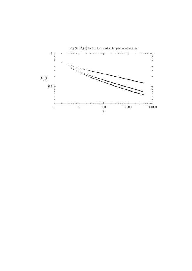
Figure 3: The global persistence probability in two dimensions for random initial conditions ($L$=199) for $m_{0}$ = 0.2, 0.1 and 0 (from top to bottom) are shown. Typically 3$\times 10^{4}$ initial configurations are generated.

We have obtained the values of $\theta_{g}$ for several values of non zero $m_{0}$ and also for $m_{0}$=0 for comparison with model A. Note that for the global persistence one needs the fraction of configurations for which the order parameter does not change sign and to get a good estimate of $\theta_{g}$ one needs to generate a large number of configurations. Thus to restrict the total computation, we have evaluated $\theta_{g}$ for a few values of $m_{0}$ only unlike the local case. Moreover, in the global case, the system is critical and estimating the critical temperature again involves a lot of computations.

The numerical values of $\theta_{g}$ for model A [6] are recovered when $m_{0}=0$ with both RP and SP initial conditions. In both two and three dimensions, the values of $\theta_{g}$ appear to depend on $m_{0}$ (see Table I). In the SP initial condition, estimation of $\theta_{g}$ becomes difficult as the fluctuations are considerable even with $3\times 10^{4}$ configurations. Hence instead of the extrapolation procedure, we give in Table I the value of $\theta_{g}$ for $m_{s}(0)=0.0005$ and $m_{s}(0)=0.0002$ in two and three dimensions respectively for which the fluctuations are minimum. For low values of $m_{0}$, $\theta_{g}$ is very close (if not equal) to the model A values with both RP and SP states. For higher values of $m_{0}$, it is different from that of model A and seems to vary with $m_{0}$. Typical variations of $P_{g}(t)$ in two and three dimensions are shown in Fig. 3 and 4. In agreement with [7], we indeed find that the model A and model C global persistence exponents are unequal even in two dimensions (if we use a large value of $m_{0}$), although in contrast to [7] we find non-univerality. This discrepancy might arise from the fact that in [7] a continuum model was considered while we have considered here a discrete system. Such discrepancies have been observed for the zero-temperature coarsening dynamics of the continuum model B and the corresponding discrete model [19].

Figure 4: Global persistence probability for sharply prepared initial condition in three dimensions for $m_{0}$ = 0.4, 0.2 and 0 (from top to bottom) with $L$=41 are plotted. Typically 3$\times 10^{4}$ initial configurations are generated.

The analytical results of model B and the present numerical results in a system belonging to model C suggest that in persistence phenomena conservation plays a key role which may be responsible for the non-universality of the exponents and it is not important whether conservation is considered in the order parameter or in a coupled non-ordering field. However, the analytical study of [7] and a recent study [20] of both the local and global persistence in an absorbing phase transition in a conserved model does not show non-universality. Therefore for a better understanding of our results it is necessary to get an analytical estimate of the local persistence behaviour in model C. Also, the global persistence may be studied in greater detail both analytically and numerically. The non-monotonic behaviour in the local persistence exponent for small $m_{0}$ is also a novel observation. In the case of global persistence, owing to the large number of configurations required to get a reliable result, we had to restrict the computations to a few values of $m_{0}$ and it was not possible to study in detail the behaviour for small $m_{0}$ where the local persistence exponent shows the anomalous behaviour.

It is also interesting to compare the local and global persistence in models A and C. In model A, in three dimensions, $\theta_{g}>\theta_{l}$. From the present study, we find that while $\theta_{l}$ increases for $m_{0}$ above a certain value, $\theta_{g}$ decreases with $m_{0}$. Hence the relation $\theta_{g}>\theta_{l}$ breaks down above a certain $m_{0}$ in model C. The exact significance of this result is yet to be understood.

Lastly, all the above results for local and glocal persistence in the antiferromagnetic Ising system with conserved magnetisation were obtained with local conservation. It is expected that non-local conservation will lead to different results.

Acknowledgements: We are greatful to S. Dasgupta for valuable discussions. PS acknowledges DST grant no SP/S2/M-11/99. The computations were done on an Origin200 in CUCC.

References

- [1] A. J. Bray, B. Derrida and C. Godreche, J. Phys. A 27, L357 (1994);
- [2] For a review, see S. N. Majumdar, Curr. Sci. India 77 370 (1999).
- [3] S.N. Majumdar, A. J. Bray, S. J. Corwell and C. Sire, Phys. Rev. Lett. 77 3704 (1996).
- [4] P.C. Hohenberg and B.I. Halperin, Rev. Mod. Phys. 49 435 (1977).
- [5] B. Derrida, V. Hakim and V. Pasquier, Phys. Rev. Lett. 75 751 (1995).
- [6] A. J. Bray, B. Derrida and C. Godreche, Eur. Phys. Lett. 27 175 (1994); D. Stauffer, J. Phys. A 27 5029 (1994); S. N. Majumdar and C. Sire, Phys. Rev. Lett. 77 1420 (1996).
- [7] K. Oerding, S. J. Cornell and A. J. Bray, Phys. Rev. E 56 R25 (1997).
- [8] L. Schuelke, B. Zheng, Phys. Lett. A 233 93 (1997).
- [9] B. P. Lee and A. D. Rutenberg, Phys. Rev. Lett. 79 4842 (1997).
- [10] A.J. Bray, Phys. Rev. Lett. 66 C2048 (1991).
- [11] C. Sire and S.N. Majumdar, Phys. Rev. E 52 244 (1995).
- [12] P. Sen, J. Phys. A 32 1623 (1999).
- [13] B. Zheng and H.J. Luo, Phys. Rev. E 63 066130 (2001).
- [14] H. K. Janssen, B. Schaub and B. Schmittmann, Z. Phys. B73 539 (1989).
- [15] K. Oerding and H.K. Janssen, J. Phys. A 26 3369 (1993).
- [16] P. Sen, S. Dasgupta and D. Stauffer, Eur. Phys. J. B 1 107 (1998).
- [17] P.Sen and S.Dasgupta, J. Phys. A 35 2755 (2002).
- [18] E. Eisenriegler and B. Schaub, Z. Phys. B 39 65 (1980).
- [19] S. Cueille and C. Sire, J. Phys. A 30 L791 (1997).
- [20] S. Lubeck and A. Misra, Eur. Phys. J. B, to be published, (cond-mat/0201411).