[

Nucleation of superconductivity in mesoscopic star-shaped superconductors

Abstract

We study the phase transition of a star-shaped superconductor, which covers smoothly the range from zero to two dimensions with respect to the superconducting coherence length $\xi(T)$. Detailed measurements and numerical calculations show that the nucleation of superconductivity in this device is very inhomogeneous, resulting in rich structure in the superconducting transition as a function of temperature and magnetic field. The superconducting order parameter is strongly enhanced and mostly robust in regions close to multiple boundaries.

]

Many characteristics of a superconducting sample are strongly influenced by its size with respect to fundamental superconducting length scales. Experimental and theoretical investigations over the past few decades have clearly delineated the differences in behavior between one-dimensional, two-dimensional and “bulk” three-dimensional samples in properties such as the critical field, critical temperature and critical current. Recently [5], there has been renewed interest in the effect of sample dimension on the properties of superconductors, fueled in part by their potential use in future nanometer scale devices. The complex geometry of such devices implies that one needs to consider the nucleation of superconductivity over a range of length scales in a single device.

The nucleation of superconductivity in the presence of a magnetic field can be investigated by solving the Ginzburg-Landau(GL) equations for the superconducting order parameter $\psi$ and the vector potential $\bf A$ of the magnetic field $\bf B=\nabla\times A$ [6, 7, 8]:

$$\frac{1}{2m}\left(-i\hbar{\bf\nabla}-\frac{2e}{c}{\bf A}\right)^{2}\psi+\alpha\psi+\beta\left|\psi\right|^{2}\psi=0,$$ (1)

$${\bf\nabla}^{2}{\bf A}=\frac{4\pi ie\hbar}{mc}\left(\psi^{\ast}{\bf\nabla}\psi-\psi{\bf\nabla}\psi^{\ast}\right)+\frac{16\pi e^{2}}{mc^{2}}{\bf A}\left|\psi\right|^{2}$$ (2)

subject to the boundary condition

$${\bf n}\cdot\lgroup-i\hbar{\bf\nabla}-\frac{2e}{c}{\bf A}\rgroup\psi=0.$$ (3)

Here $\alpha$ and $\beta$ is the GL parameters, and $\bf n$ is the unit vector normal to the surface.

Close to the critical temperature $T_{c}$, $\left|\psi\right|^{2}$ is negligible, and one can analytically solve the linearized GL equation (1) for some simple geometries. Saint-James and de Gennes[9] solved this linear equation for the case of a magnetic field parallel to the surface of a superconductor. They found that superconductivity could exist at a field $H_{c3}$ (the so-called surface critical field) larger than the upper critical field $H_{c2}$ in the bulk superconductor, $H_{c3}=1.69H_{c2}$. More recently[10, 11, 12], attention has focused on superconducting wedges subtending an angle $\gamma$, with the magnetic field applied parallel to the wedge’s edge. In the limit of small $\gamma$, it has been predicted[13, 14] that the surface critical field can be greatly enhanced, $H_{c3}=(1.73/\gamma)H_{c2}$, although this has never been demonstrated experimentally. This large enhancement of $H_{c3}$ can be ultimately traced to the increase in the “energy” ($-\alpha$) in the GL equation (1) associated with the confinement of the order parameter.

For more complicated geometries, and for regimes further away from the superconducting transition, it is necessary to solve the full GL equations numerically. This has been done for many different geometries, including wedges, rings[15, 16], square loops[17, 18] and bridges[19]. Here we are interested in a four-pointed “star” geometry, shown schematically in Fig. 1. The remarkable feature of this geometry is that it encompasses a wide range of length scales. As we shall see, this results in appearance of regions of the sample with characteristically different behavior in the superconducting regime.

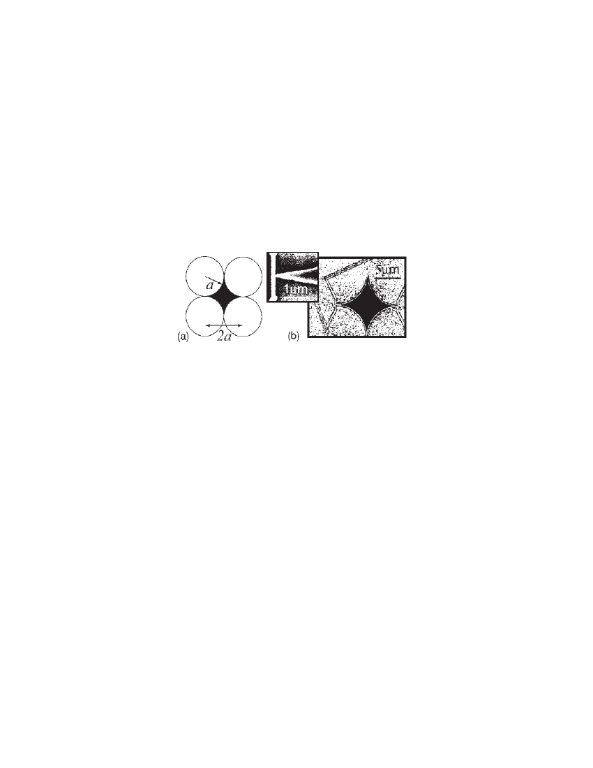
FIG. 1.: (a) Schematic representation of the method that was used to design samples. (b) Scanning electron micrograph of one of the samples. The inset shows magnified area of the apex.

The experimental sample is prepared by removing portions of a circle of radius $a$ from the corners of a square of side $2a$, as shown in Fig. 1 (a). The experimental realization of this geometry is shown in Fig. 1(b). The sample is fabricated by conventional electron beam lithography with a 60 nm thick Al film. The apex-to-apex distance is 12 $\mu$m, the minimum dimension at each apex is less than 100 nm. These dimensions are also used in all numerical calculations. In order to enable four terminal electrical measurements on the device, narrow electrical contacts of the same material are attached to opposite apices.

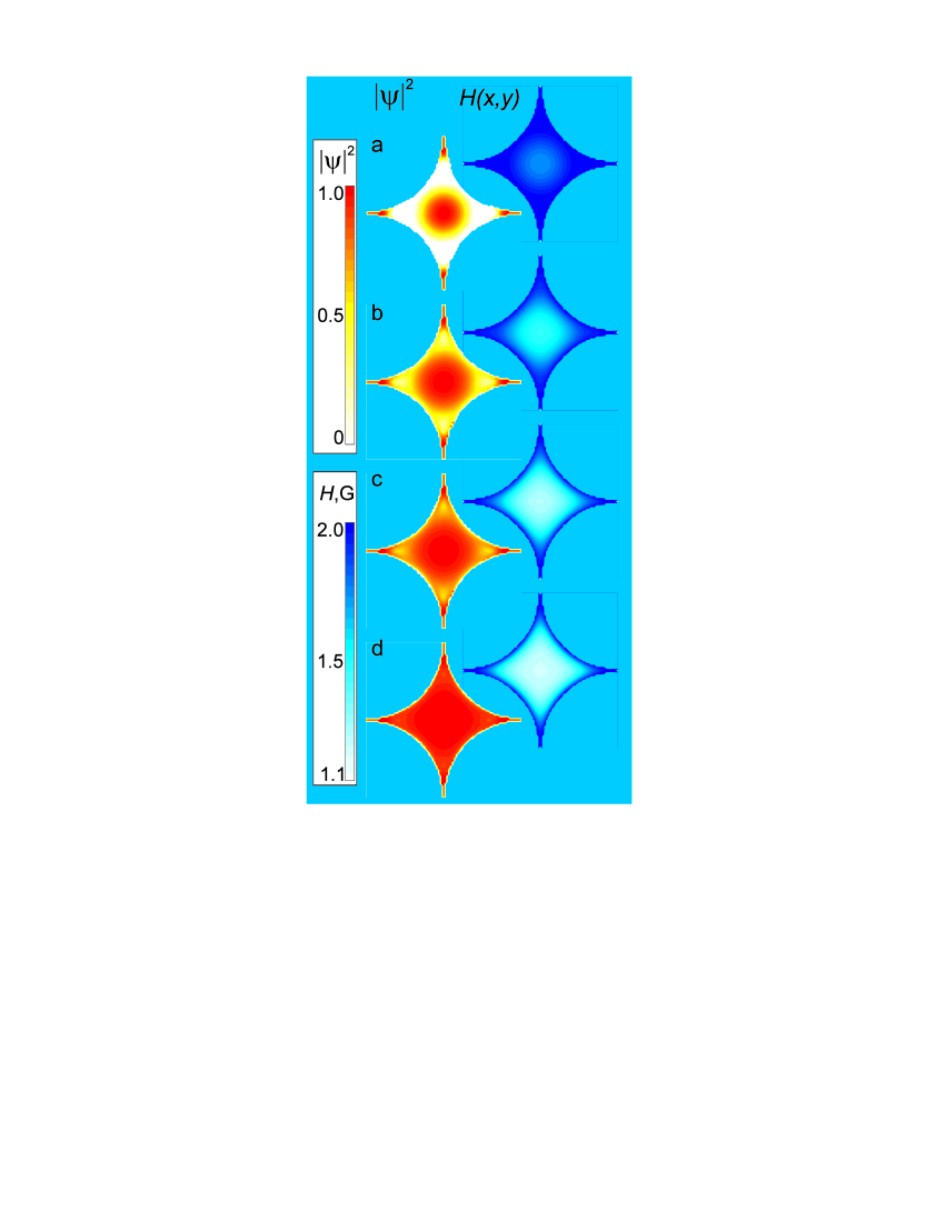
FIG. 2.: Evolution of $\left|\psi(x,y)\right|^{2}$ and magnetic field distribution in the star with temperature for an applied external field of $H_{0}=0.02H_{c}(0)$ = 2 G, where $H_{c}(0)$ = 100 G is the bulk critical field at zero temperature, at different temperatures: a - $T/T_{c}$ = 0.99, b - 0.98, c - 0.97, d - 0.94. $\left|\psi(x,y)\right|^{2}$ is normalized to its maximum value at these temperatures.

To obtain the solutions of the GL equations (1), (2) with the boundary conditions (3), we use the finite-difference method applied earlier for the description of superconductivity in a mesoscopic square loop[17, 18], using the dimensions and parameters of the experimental sample of Fig. 1. One additional complication of this geometry for the finite-difference method is the infinite sharpness of the apices of the star, which makes the generation of a mesh for the problem difficult. Fortunately, the vertices of the experimental sample have finite curvature, which results in a definite cut-off length of around 100 nm for the tip of each apex, as shown in the small inset to Fig. 1. In our calculations of the order parameter and magnetic field distributions, a square mesh has been used with the density of 800 nodes per side of the sample. At such a high density of nodes, the results of calculations are independent of the mesh.

The solutions of the GL equations with appropriate boundary conditions permit us to obtain the spatial distribution of the order parameter and the magnetic field as a function of temperature $T$, as shown in Fig. 2. As temperature is decreased slightly from $T_{c}\,\ (T/T_{c}=0.99)$, one observes nucleation of superconductivity as evidenced by a non-zero $\left|\psi(x,y)\right|^{2}$ in two distinct regions of the sample. The first region is a large area in the center, where one might intuitively expect superconductivity to nucleate. The second region is at the apices of the star, where superconductivity is enhanced by the close proximity of two boundaries, and resembles the situation that occurs in a superconducting “wedge.” In between these two regions, $\left|\psi\right|^{2}$ is essentially 0, so that the superconducting phases of the sample are separated by regions of normal phase. The plot of the field distribution shows that the two superconducting regions are characterized by different behavior in a magnetic field: the central region shows the beginning of Meissner expulsion of the external field, while the magnetic field near the boundaries is very close to the external field value. As the temperature is lowered further, the superconducting areas in the two regions grow as expected to cover almost the entire sample, and the normal regions between the apices and the center disappear. At the lowest temperature shown, the value of $\left|\psi\right|^{2}$ at the apices and in the central region achieves its maximum value corresponding to this temperature, $\left|\psi(x,y)\right|^{2}_{max}\sim(1-T/T_{c})=0.06$. The magnetic field at the center is greatly reduced, showing the presence of a strong Meissner effect, but the magnetic field in a narrow region at the boundaries of the sample is still very close to the external field value. It should be noted that the value of $\left|\psi\right|^{2}$ at the apices is a maximum, even though the magnetic field is also a maximum. In fact, the value of $\left|\psi\right|^{2}$ at the apices does not change appreciably over the temperature range shown in Fig. 2, demonstrating vividly the fact that superconductivity is the most robust in regions close to multiple boundaries.

The electrical contacts in the sample are placed at opposite apices, so that the electrical current must traverse these apices, the central region, as well as any normal regions in between. Consequently, the inhomogeneous nature of superconductivity nucleation as the sample is cooled through its transition imparts a distinctive shape

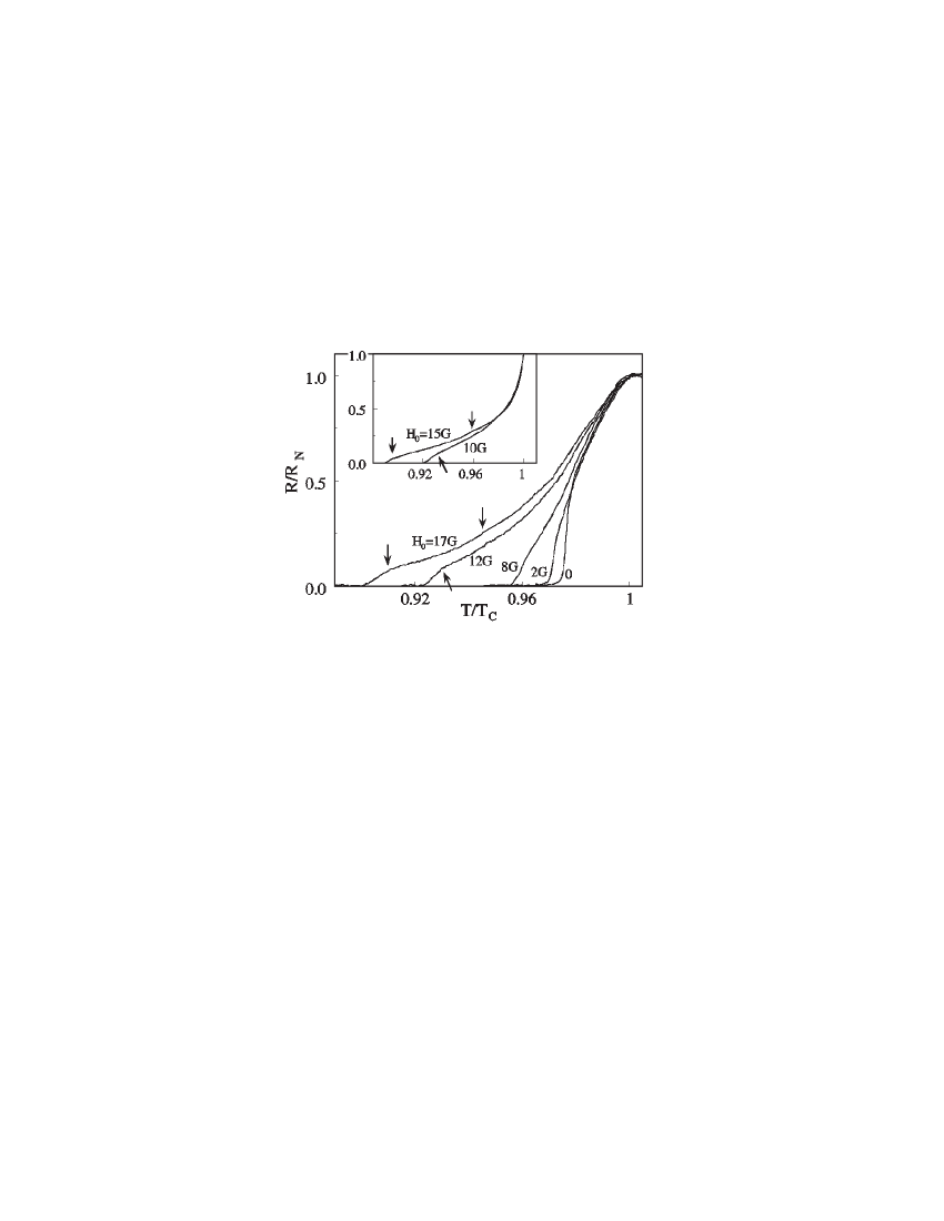
FIG. 3.: Experimentally measured resistive transition, taken at different magnetic fields. The inset shows the numerically calculated $R(T)$. $T_{c}$ = 1.32 K, and $R_{N}$ = 12 $\Omega$.

to $R(T)$, as shown in Fig. 3. The normal-to-superconducting transition starts with a decrease in resistance over a relatively broad range in temperature even at $H_{0}=0$. In this temperature range, superconductivity begins to nucleate at the apices and at the central part, as was shown in Fig. 2, but the regions near the apices, being narrower, contribute a large fraction to the resistance change. As the temperature is reduced further, there is a much sharper drop in the resistance when $R$ is a little less than half the normal state resistance $R_{N}$. Since the central region and the apices are already superconducting, this rapid change corresponds to the normal-to-superconducting transition of the “necks” between the apices and the central region. Calculations of the superconducting transition confirm this picture.

Numerically, we calculate the resistance of the sample using the order parameter distribution. As the order parameter and magnetic field distributions, the resistance of the sample is calculated on a rectangular mesh. The resistance of a mesh cell in the sample is determined by the value of $\left|\psi(x,y)\right|^{2}$ in the cell, being zero if $\left|\psi(x,y)\right|^{2}>0$, and equal to the normal state resistance if $\left|\psi(x,y)\right|^{2}=0$. One must also take into account the Josephson coupling between the superconducting regions, which reduces the resistance of the “necks”. We suppose that a region of the normal metal of length $\leq p\cdot\xi$ (where $p\approx 2$ is an adjustable parameter) between superconducting “islands” does not contribute to the resistance in the circuit. The inset of Fig. 3 shows result of this calculation for two different field values. The theoretical curves reproduce the main qualitative features of the experimental curves, including the “kinks” (denoted by the arrows) at lower resistance, and are in reasonably good quantitative agreement as well. The calculated position of the beginning of the resistive transition compares rather well with the experimental curves when the tunneling of the superconducting electrons through the normal metal is taken into consideration.

The behavior of the sample in a magnetic field (Fig. 4) exhibits even more distinctly the difference between the nature of the superconductivity in the center and the apices. While $\left|\psi(x,y)\right|^{2}$ in the central region is rapidly attenuated with increasing magnetic field, its value in the apices does not show a large change. At large magnetic fields, only the apices are superconducting. This would imply that the contribution to the resistance of the sample from the apices is not strongly affected by magnetic field. Evidence for this can be seen directly in the experimental transition curves. The resistance of the sample at the top of the transition, where the decrease in resistance is primarily due to the nucleation of superconductivity in the apices, shows only a weak dependence on magnetic field. At lower values of resistance, where one has contributions from the central region as well as the “necks”, the field dependence is much stronger, reflecting the two-dimensional nature of the superconductivity in these regions.

Even more striking is the magnetic phase diagram ($T_{c}$ vs. $H$) of the sample. Typically, this is obtained by varying the temperature to maintain the resistance of the sample at the midpoint of the transition ($R/R_{N}=0.5$) while changing the magnetic field. Since our sample is inhomogeneous, and it is not clear how one would define the unique $T_{c}$, we have measured the phase diagram with the sample biased at various points $R/R_{N}$ of the superconducting transition. Figure 5 shows the result of these measurements. Although the curves are different, each one shows two distinct regions, separated by a well-defined “kink” denoted by the arrow. At low fields, the curves show a quasi-linear dependence on $H_{0}$, which turns into a quadratic dependence at higher magnetic fields. It is well known that the critical temperature of a superconductor varies linearly with the magnetic field in two dimensions, and quadratically in one dimension[8]. The “kink” in each curve defines the crossover from two-dimensional behavior at low fields to one-dimensional behavior at higher fields. This behavior is in agreement with the evolution of the superconducting regions of the sample shown in the numerical simulations of Fig. 3. At low fields, the central region and the “necks” of the sample are superconducting, giving a two-dimensional characteristic to the phase diagram. At higher fields, superconductivity in these regions is attenuated, leaving a finite order parameter only in the apices, which gives rise to a quadratic dependence on the magnetic field. It is interesting to note that the low-field linear behavior of all the curves extrapolates to a single temperature at $H_{0}=0$, while the high-field quadratic behavior of all the curves also extrapolates to a single (but different) temperature. The different temperatures clearly point out the inhomogeneous nature of the superconducting transition in this device.

[

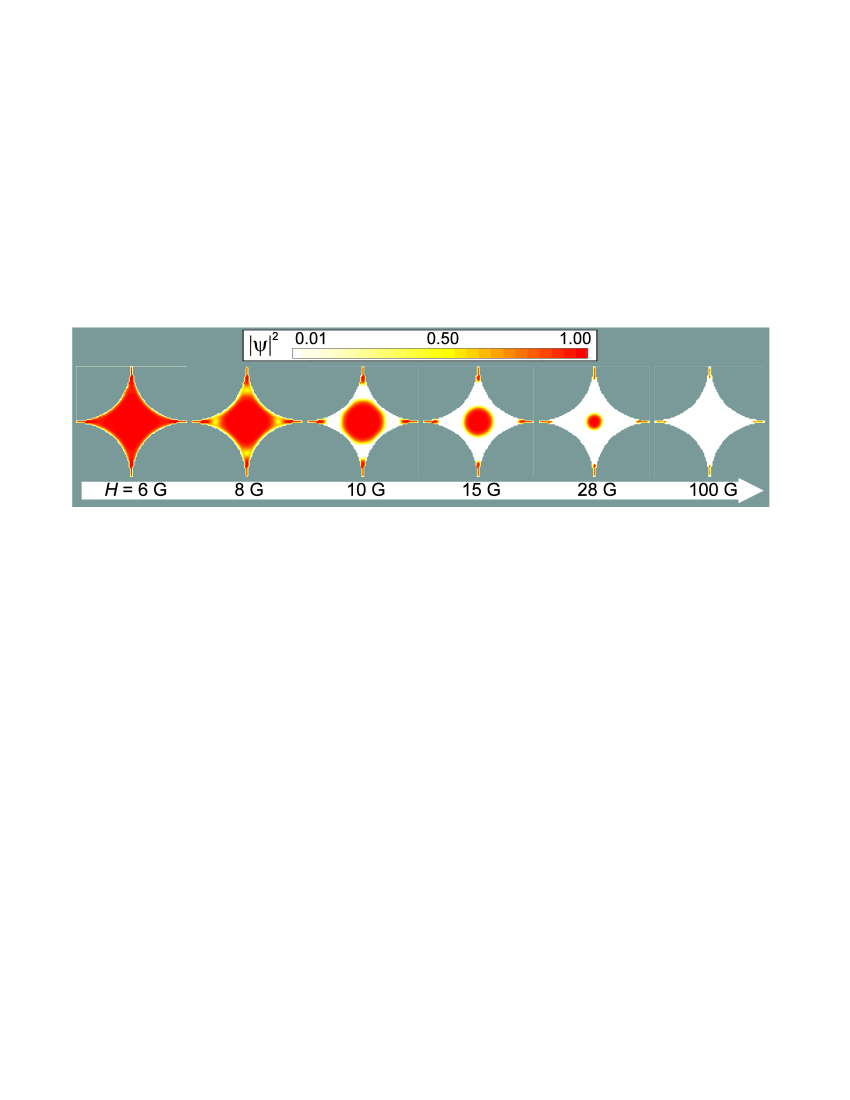
FIG. 4.: Evolution of $\left|\psi(x,y)\right|^{2}$ with magnetic field at $T/T_{c}$ = 0.8. $\left|\psi(x,y)\right|^{2}$ is normalized to its maximum value at this temperature.

]

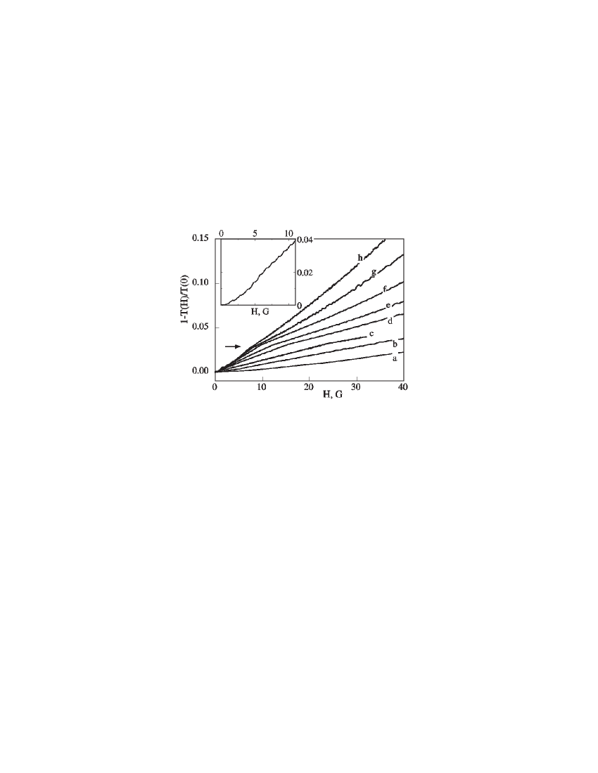
FIG. 5.: $T-H$ phase diagrams measured at $R/R_{N}$ = 0.58 (a), 0.42 (b), 0.33 (c), 0.25 (d), 0.21 (e), 0.17 (f), 0.125 (g), 0.08 (h). Inset shows the Little-Parks[20] oscillations at smaller field for $R/R_{N}$ = 0.04.

In conclusion, we have analyzed the resistive transition in a star-shaped sample, which combines properties of two-dimensional and zero-dimensional superconductors in a unique manner. Occurrence of qualitatively different regions in the resistive transition reflects a smooth change from 2D to 0D superconducting regime when increasing applied magnetic field or temperature.

We thank V. V. Moshchalkov for valuable discussions. This work was supported at Northwestern University by the National Science Foundation through grant DMR-0201530 and by the David and Lucile Packard Foundation, and at Universiteit Antwerpen by the IUAP, the GOA BOF UA, the FWO-V, WOG (Belgium) and the ESF Programme VORTEX.

REFERENCES

- [1] Permanent address: Institute for Low Temperature Physics and Engineering, 61164 Kharkov, Ukraine.
- [2] Permanent address: Institute of Applied Physics, MD-2028 Kishinev, Republic of Moldova.
- [3] Permanent address: Department of Theoretical Physics, State University of Moldova, MD-2009 Kishinev, Republic of Moldova.
- [4] Also at Universiteit Antwerpen (RUCA), B-2020 Antwerpen, Belgium and Technische Universiteit Eindhoven, 5600 MB Eindhoven, The Netherlands.
- [5] V. V. Moshchalkov, L. Gielen, C. Strunk, R. Jonckheere, X. Qiu, C. Van Haesendonck, Y. Bruynseraede, Nature 373, 319 (1995).
- [6] V. L. Ginzburg, L. D. Landau, Zh. Eksp. Teor. Fiz. 20, 1064 (1950).
- [7] P. G. de Gennes, Superconductivity of Metals and Alloys, [Addison-Wesley Publishing Company, Massachusetts, 1989].
- [8] M. Tinkham, Introduction to Superconductivity, 2nd edition, [McGraw Hill, New York, 1996].
- [9] D. Saint-James, P. G. de Gennes, Phys. Lett. 7, 306 (1963).
- [10] V. M. Fomin, J. T. Devreese, V. V. Moshchalkov, Europhys. Lett. 42, 553 (1998); 46, 118 (1999).
- [11] F. Brosens, J. T. Devreese, V. M. Fomin, V. V. Moshchalkov, Solid State Commun. 111, 565 (1999).
- [12] S. N. Klimin, V. M. Fomin, J. T. Devreese, V. V. Moshchalkov, Solid State Commun. 111, 589 (1999).
- [13] A. Houghton, F. B. McLean, Phys. Lett. 19, 172 (1965).
- [14] A. P. Van Gelder, Phys. Rev. Lett. 20, 1435 (1968).
- [15] V. A. Schweigert, F. M. Peeters, P. S. Deo, Phys. Rev. Lett. 81, 2783 (1998).
- [16] V. A. Schweigert, F. M. Peeters, Phys. Rev. B 60, 3084 (1999).
- [17] V. M. Fomin, V. R. Misko, J. T. Devreese, V. V. Moshchalkov, Solid State Comm. 101, 303 (1997).
- [18] V. M. Fomin, V. R. Misko, J. T. Devreese, V. V. Moshchalkov, Phys. Rev. B 58, 11703 (1998).
- [19] V. R. Misko, V. M. Fomin, J. T. Devreese, Phys. Rev. B 64, 014517 (2001).
- [20] W. A. Little, R. D. Parks, Phys. Rev. Lett. 9, 9 (1962).