Thermodynamic properties of the SO(5) model of high-$T_{c}$ superconductivity

Abstract

In this paper we present calculations of thermodynamic functions within Zhang’s SO(5) quantum rotor theory of high-$T_{c}$ superconductivity. Using the spherical approach for the three-dimensional quantum rotors we derieved explicit analytical formulas for entropy and specific heat related to the lattice version of the SO(5) nonlinear quantum-sigma model. We present the temperature dependence of these quantities for various settings of relevant control parameters (quantum fluctuations, chemical potential). We find our results in overal qualitative agreement with basic thermodynamics of high-$T_{c}$ cuprates.

I Introduction

The theory unifying antiferromagnetism (AF) and superconductivity (SC) to describe global phase diagram of high-$T_{c}$ superconductors was recently proposed by Zhang. ZhangScience In this approach, based on symmetry principles, a three-dimensional order parameter (the staggered magnetization) describing the AF phase and a complex order parameter (with two real components), describing a spin singlet d-wave SC phase are grouped in five-component vector called a “superspin”. The SO(3) symmetry of spin rotations (which is spontaneously broken in the AF phase) and the electro-magnetic SO(2) invariance (whose breaking defines SC phase) along with well-defined AF to SC and vice versa rotation operators form SO(5) symmetry. In the Zhang’s theory both ordered phase arise once SO(5) is spontaneously broken and the competition between antiferromagnetism and superconductivity is related to direction of the “superspin”in the five-dimensional space. The low energy dynamics of the system is determined in terms of the Goldstone bosons and their interactions specified by the SO(5) symmetry. The kinetic energy of the system is that of a SO(5) rigid rotor and the system is described by a SO(5) non-linear quantum $\sigma$ model (NLQ$\sigma$M). The SO(5) quantum rotor model offers a Landau-Ginzburg-like (LG) approach for the high-$T_{c}$ problem. However, it goes much beyond the traditional LG theory, since it captures dynamics. While the SO(5) symmetry was originally proposed in the context of an effective field-theory description of the high-$T_{c}$ superconductors, its prediction can also be tested within microscopic models. MicroscopicModels1 ; MicroscopicModels2 ; MicroscopicModels3 ; MicroscopicModels4 ; MicroscopicModels5 ; Arrigoni For example, numerical evidence for approximate SO(5) symmetry of the Hubbard model came out from exact diagonalization of small sized clusters. Meixner The global features of the phase diagram deduced from SO(5) theory based on a spherical quantum rotors PRB1 agree qualitatively with the general topology of the observed phase diagram of high-$T_{c}$ superconductors. The quantitative investigation of the quantum critical point scenario within the concept of the SO(5) group, e.g. the scaling of the contribution to the electrical resistivity due spin fluctuations showed linear resistivity dependence on temperature for increasing quantum fluctuation – being a hallmark example of anomalous properties in cuprate materials. PRL The systematic studies of magnetic properties of the SO(5) theory showed that the theory yields a qualitative scenario for the evolution of magnetic behavior, which is consistent with experiments. PRB2 It qualitatively explains the results of experimental measurements (notably the NMR relaxation rates) with correct predictions of behavior of uniform spin susceptibility in high temperatures. Also the energy dependence of the momentum-integrated dynamic spin susceptibility show features, which are in qualitative agreement with experimental findings.

Thermal fluctuations are pronounced in the high-$T_{c}$ superconductors due to number of reasons. The carrier density is rather small, the anisotropy is large and the critical temperature is high. It turns out that deviations from the mean-field behavior are present in the specific heat $C$ at the superconducting transition temperature $T_{c}$. In the mean-field BCS theory, a second order transition with a jump in a specific heat at $T_{c}$ takes place. In contrary, in most high-$T_{c}$ superconductors thermal fluctuations seem to restore common behavior.

The aim of the present paper is to study quantitatively basic thermodynamic functions resulting from the SO(5) theory, thereby substantiating this theoretical framework. Our study may also provide a useful diagnostic tool for testing the basic principles of SO(5) theory by comparing the quantitative predictions (e.g., specific heat) with the outcome of the relevant experiments.

The outline of the reminder of the paper is as follows. In Section II we begin by setting up the quantum SO(5) Hamiltonian and the corresponding Lagrangian. In Section III we find closed forms of various thermodynamic functions. We calculate free energy, entropy and specific heat. Finally, in Section IV we summarize the conclusions to be drawn from out work.

II Hamiltonian and the effective Lagrangian

We consider the low-energy Hamiltonian of superspins placed in the nodes of a discrete three dimensional simple cubic (3DSC) lattice,

$$H = \frac{1}{2u}\sum_{i}\sum_{\mu<\nu}L_{i}^{\mu\nu}L_{i}^{\mu\nu}-\sum_{i<j}J_{ij}\mathbf{n}_{i}\cdot\mathbf{n}_{j}+$$ (1)

$$-V\left(\mathbf{n}_{i}\right)-2\mu\sum_{i}L_{i}^{15}\text{.}$$

Indices $i$ and $j$ number lattice sites running from $1$ to $N$ - the total number of sites, while $\mu$,$\nu=1,...,5$ denote superspin $\mathbf{n}_{i}=\left(n_{1},n_{2},n_{3},n_{4},n_{5}\right)_{i}$ components ($\mathbf{n}_{AF,i}=\left(n_{2},n_{3},n_{4}\right)_{i}$ refers to antiferromagnetic and $\mathbf{n}_{SC,i}=\left(n_{1},n_{5}\right)_{i}$ superconducting order, respectively). The superspin components are mutually commuting (according to Zhang’s formulation) and their values are restricted by the rigidity constraint $\mathbf{n}_{i}^{2}=1$.

The first part of the equation (1) is the kinetic energy of the system (being simply that of a SO(5) rigid rotor), where

$$L_{i}^{\mu\nu}=n_{\mu i}p_{\nu i}-n_{\nu i}p_{\mu i}$$ (2)

are generators of Lie SO(5) algebra (expressed by total charge $L_{i}^{15}$, spin and so-called “$\pi$”operators), $p_{\mu i}$ are momenta conjugated to respective superspin components:

$$p_{\mu i}=i\frac{\partial}{\partial n_{\mu i}},$$

$$\left[n_{\mu},p_{\nu}\right]=i\delta_{\mu\nu}$$ (3)

and parameter $u$ measures the kinetic energy of the rotors (an analog of moment of inertia).

The second part of the Hamiltonian is the inter-superspin interaction energy with $J$ being the stiffness in the charge and spin channel. In the 3DSC lattice, $J$ is nonvanishing for the nearest neighbors and its Fourier transform

$$J_{\mathbf{q}}=\frac{1}{N}\sum_{\mathbf{R}_{i}}J\left(\mathbf{R}_{i}\right)e^{-i\mathbf{R}_{i}\cdot\mathbf{q}}$$ (4)

is simply

$$J_{\mathbf{q}}/J=\cos q_{x}+\cos q_{y}+\cos q_{z}.$$ (5)

For convenience, we will further introduce the density of states

$$\rho\left(\xi\right)=\frac{1}{N}\sum_{\mathbf{q}}\delta\left(\xi-J_{\mathbf{q}}/J\right)\text{,}$$ (6)

which for 3DSC3d lattice reads:

$$\rho\left(\xi\right) = \frac{1}{\pi^{3}}\int_{\max(-1,-2-\xi)}^{\min(1,2-\xi)}\frac{dy}{\sqrt{1-y^{2}}}\times$$ (7)

$$\times\mathbf{K}\left[\sqrt{1-\left(\frac{\xi+y}{2}\right)^{2}}\right]\Theta\left(3-\left|\xi\right|\right)\text{,}$$

where $\mathbf{K}\left(x\right)$ is the elliptic integral of the first kind and $\Theta\left(x\right)$ is the step function EllipticFunction .

The last two parts of the equation (1) provide symmetry SO(5) breaking terms. In the result of their interplay, the system favours either the “easy plane”in the superconducting (SC) space $\left(n_{1},n_{5}\right)$, or an “easy sphere”in the antiferromagnetic (AF) space $\left(n_{2},n_{3},n_{4}\right)$. The first of two terms is defined as:

$$V\left(\mathbf{n}_{i}\right)=\frac{w}{2}\sum_{i}\left(n_{2i}^{2}+n_{3i}^{2}+n_{4i}^{2}\right),$$ (8)

with the anisotropy constant $w$, which positive value favours AF state. The second term contains a charge operator $L_{i}^{15}$, whose expectation value yields the doping concentration and the chemical potential $\mu$ (measured from the half-filling), whose positive values favour SC state.

The partition function $Z=Tre^{-H/k_{B}T}$ is expressed using the functional integral in the Matsubara “imaginary time”$\tau$ formulation PRB1 ($0\leq\tau\leq 1/k_{B}T\equiv\beta$, with $T$ being the temperature). We obtain:

$$Z = \int\prod_{i}\left[D\mathbf{n}_{i}\right]\int\prod_{i}\left[\frac{D\mathbf{p}_{i}}{2\pi}\right]\delta\left(1-\mathbf{n}_{i}^{2}\right)\delta\left(\mathbf{n}_{i}\cdot\mathbf{p}_{i}\right)\times$$ (9)

$$\times e^{-\int_{0}^{\beta}d\tau\left[i\mathbf{p}\left(\tau\right)\cdot\frac{d}{d\tau}\mathbf{n}\left(\tau\right)+H\left(\mathbf{n},\mathbf{p}\right)\right]}=$$

$$= \int\prod_{i}\left[D\mathbf{n}_{i}\right]\delta\left(1-\mathbf{n}_{i}^{2}\right)e^{-\int_{0}^{\beta}d\tau\mathcal{L}\left(\mathbf{n}\right)},$$

with $\mathcal{L}$ being the Lagrangian:

$$\mathcal{L}\left(\mathbf{n}\right) = \frac{1}{2}\sum_{i}\left[u\left(\frac{\partial\mathbf{n}_{SC}}{\partial\tau}\right)^{2}+u\left(\frac{\partial\mathbf{n}_{AF}}{\partial\tau}\right)^{2}+\right.$$ (10)

$$\left.-4u\mu^{2}\mathbf{n}_{SC}^{2}+4iu\mu\left(\frac{\partial n_{1}}{\partial\tau}n_{5}-\frac{\partial n_{5}}{\partial\tau}n_{1}\right)\right]+$$

$$-\sum_{i<j}J_{ij}\mathbf{n}_{i}\cdot\mathbf{n}_{j}-\frac{w}{2}\sum_{i}\left(n_{2i}^{2}+n_{3i}^{2}+n_{4i}^{2}\right)\text{.}$$

The problem can be solved exactly in terms of the spherical modelSphere . To accommodate this we notice that the superspin rigidity constraint ($\mathbf{n}_{i}^{2}=1$ ) implies that a weaker condition also holds, namely:

$$\sum_{i=1}^{N}\mathbf{n}_{i}^{2}=N\text{.}$$ (11)

Therefore, the superspin components $\mathbf{n}_{i}\left(\tau\right)$ must be treated as $c$-number fields, which satisfy the quantum periodic boundary condition $\mathbf{n}_{i}\left(\beta\right)=\mathbf{n}_{i}\left(0\right)$ and are taken as continuous variables, i.e., $-\infty<\mathbf{n}_{i}\left(\tau\right)<\infty$, but constrained (on average, due to Eq. (11)) to have unit length.

This introduces the Lagrange multiplier $\lambda\left(\tau\right)$ adding an additional quadratic term (in $\mathbf{n}_{i}$ fields) to the Lagrangian (10). Fourier transform $\mathbf{n}(\mathbf{k},\omega_{\ell})$ of the superspin components

$$\mathbf{n}_{i}\left(\tau\right)=\frac{1}{\beta N}\sum_{\mathbf{k}}\sum_{\ell=-\infty}^{\infty}\mathbf{n}\left(\mathbf{k},\omega_{\ell}\right)e^{-i\left(\omega_{\ell}\tau-\mathbf{k\cdot r}_{i}\right)}$$ (12)

introduces the Matsubara (Bose) frequencies $\omega_{\ell}=2\pi\ell/\beta$ ($\ell=0,\pm 1,\pm 2,...$).

Using the Eq. (9), the partition function can be written in the form:

$$Z=\int\frac{d\lambda}{2\pi i}e^{-N\phi\left(\lambda\right)}\text{,}$$ (13)

where the function $\phi\left(\lambda\right)$ is defined as:

$$\phi\left(\lambda\right) = -\int_{0}^{\beta}d\tau\lambda\left(\tau\right)-\frac{1}{N}\ln\int\prod_{i}\left[D\mathbf{n}_{i}\right]\times$$ (14)

$$\times\exp\left[-\sum_{i}\int_{0}^{\beta}d\tau\left(\mathbf{n}_{i}^{2}\lambda\left(\tau\right)-\mathcal{L}\left[\mathbf{n}\right]\right)\right]\text{.}$$

The exact value of the partition function can be found in the thermodynamic limit ($N\rightarrow\infty$), when the method of steepest descents is exact and the saddle point $\lambda\left(\tau\right)=\lambda_{0}$ satisfies the condition:

$$\left.\frac{\delta\phi\left(\lambda\right)}{\delta\lambda\left(\tau\right)}\right|_{\lambda=\lambda_{0}}=0\text{.}$$ (15)

At criticality, corresponding order parameters susceptibilities becomes infinite and corresponding Lagrange multipliers are:

$$\lambda_{0}^{AF} = \frac{1}{2}J_{\mathbf{k}=0}+\frac{w}{2},$$

$$\lambda_{0}^{SC} = \frac{1}{2}J_{\mathbf{k}=0}+2\chi\mu^{2},$$ (16)

for AF and SC critical lines, respectively. Furthermore, using the spherical condition (11) and the values (16), we finally arrive at the expression for the critical lines separating AF, SC and QD (quantum disordered) states (for more specific description these calculations see, Ref. PRB1, ; PRB2, ).

III Thermodynamic functions

III.1 Free energy

The free energy is defined as $f=-\left(\beta N\right)^{-1}\ln Z=\left(\beta\right)^{-1}\phi\left(\lambda_{0}\right)$. Using the formula (14), we obtain:

$$f = -\lambda+\frac{3}{2\beta N}\sum_{\mathbf{k},\ell}\ln\left[2\lambda-J_{\mathbf{k}}+u\omega_{\ell}^{2}-w\right]+$$

$$+\frac{1}{2\beta N}\sum_{\mathbf{k},\ell}\ln\left[2\lambda-J_{\mathbf{k}}+u\left(\omega_{\ell}+2i\mu\right)^{2}\right]+\frac{1}{2\beta N}\sum_{\mathbf{k},\ell}\ln\left[2\lambda-J_{\mathbf{k}}+u\left(\omega_{\ell}-2i\mu\right)^{2}\right]\text{.}$$

After performing the summation over Matsubara’s frequencies, we obtain the free energy:

$$f = -\lambda+\frac{1}{\beta}\int_{-\infty}^{\infty}\rho\left(\xi\right)d\xi\left\{3\ln 2\sinh\left(\frac{\beta}{2}\sqrt{\frac{2\lambda-J\xi-w}{u}}\right)\right.+$$

$$+\ln 2\sinh\left[\frac{\beta}{2}\left(\sqrt{\frac{2\lambda-J\xi}{u}}-2\mu\right)\right]$$

$$+\left.\ln 2\sinh\left[\frac{\beta}{2}\left(\sqrt{\frac{2\lambda-J\xi}{u}}+2\mu\right)\right]\right\}.$$

III.2 Entropy

The entropy is defined as $S=k_{B}\beta^{2}\frac{\partial f}{\partial\beta}$. Using the formula (III.1) we obtain:

$$S\left(\beta\right) = \frac{k_{B}}{2}\int_{-\infty}^{\infty}\rho\left(\xi\right)d\xi\left\{3\left[\beta A\left(\xi\right)\coth\frac{\beta}{2}A\left(\xi\right)-2\ln 2\sinh\frac{\beta}{2}A\left(\xi\right)\right]+\right.$$

$$+\left[\beta B_{-}\left(\xi\right)\coth\frac{\beta}{2}B_{-}\left(\xi\right)-2\ln 2\sinh\frac{\beta}{2}B_{-}\left(\xi\right)\right]$$

$$+\left.\left[\beta B_{+}\left(\xi\right)\coth\frac{\beta}{2}B_{+}\left(\xi\right)-2\ln 2\sinh\frac{\beta}{2}B_{+}\left(\xi\right)\right]\right\},$$

where:

$$A\left(\xi\right) = \sqrt{\frac{2\lambda-J\xi-w}{u}},$$

$$B_{-}\left(\xi\right) = \sqrt{\frac{2\lambda-J\xi}{u}}-2\mu,$$

$$B_{+}\left(\xi\right) = \sqrt{\frac{2\lambda-J\xi}{u}}+2\mu.$$ (20)

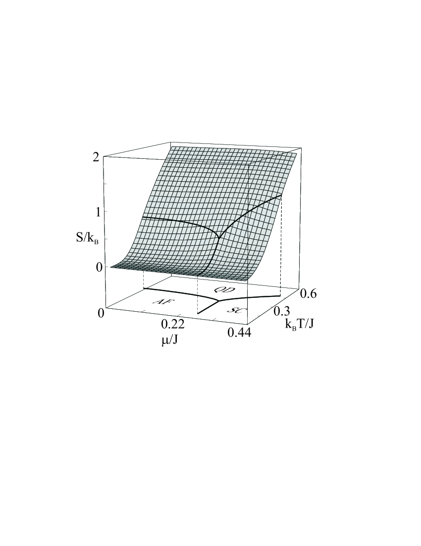
Figure 1: Plot of the entropy $S$ vs. chemical potential $\mu/J$ and temperature $k_{B}T/J$ for fixed $uJ=3$ and $w/J=1$. Solid lines indicate the projection of the $\mu-T$ phase diagram.

The dependence of the entropy on temperature and chemical-potential is shown on Fig. 1. Starting from $T=0$, the entropy increases in any ordered phase (AF or SC) until reaching $T_{c}$ (or $T_{N}$). The further increase is slower, but saturation in higher temperatures is not observed. The absolute value of the entropy is lower for higher quantum fluctuation (see, Fig. 2). We find obtained results in qualitative agreement with experimentally measured properties of high-$T_{c}$ superconductors (e.g. for Bi2212 compound, see Ref. Loram_Entropy, ).

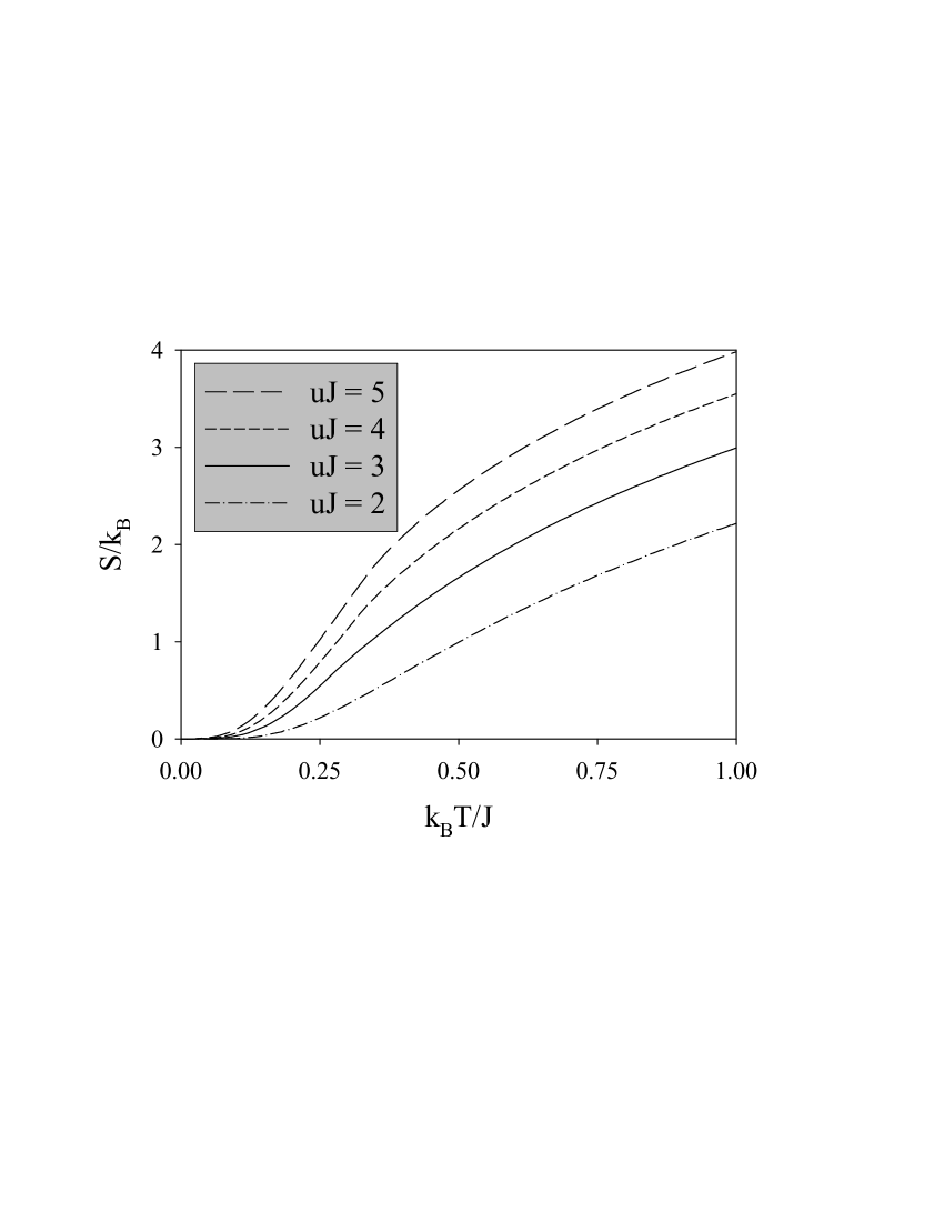
Figure 2: Plot of the entropy $S$ vs. temperature $k_{B}T/J$ for $w/J=1$, $\mu/J=0.2$ and different values of $uJ$, as indicated in the inset.

III.3 Specific heat

The specific heat at constant volume is defined:

$$C = -k_{B}\beta^{2}\frac{\partial^{2}}{\partial\beta^{2}}\left(\beta f\right)=-k_{B}\beta^{2}\left\{2\frac{\partial f}{\partial\beta}+\beta\frac{\partial^{2}f}{\partial\beta^{2}}\right.$$ (21)

$$\left.+\beta\frac{d\lambda}{d\beta}\left[\frac{\partial^{2}f}{\partial\lambda^{2}}\frac{d\lambda}{d\beta}+2\frac{\partial^{2}f}{\partial\lambda\partial\beta}\right]\right\}.$$

The derivative $d\lambda/d\beta$ can be found from the saddle-point condition (15):

$$\left.\frac{\partial f\left[\lambda\left(\beta\right),\beta\right]}{\partial\lambda}\right|_{\lambda=\lambda_{0}}=0.$$ (22)

Explicitly, we obtain:

$$\frac{d\lambda}{d\beta}=-\frac{\frac{\partial^{2}f}{\partial\lambda\partial\beta}}{\frac{\partial^{2}f}{\partial\lambda^{2}}}.$$ (23)

The specific heat:

$$C=-k_{B}\beta^{2}\left[2\frac{\partial f}{\partial\beta}+\beta\frac{\partial^{2}f}{\partial\beta^{2}}+\beta\frac{d\lambda}{d\beta}\frac{\partial^{2}f}{\partial\lambda\partial\beta}\right].$$ (24)

Using the formula (III.1) we obtain:

$$C = \frac{k_{B}\beta^{2}}{4}\int_{-\infty}^{\infty}\rho\left(\xi\right)d\xi\times$$ (25)

$$\times\left\{3A^{2}\left(\xi\right)\sinh^{-2}\frac{\beta}{2}A\left(\xi\right)+B_{-}^{2}\left(\xi\right)\sinh^{-2}\frac{\beta}{2}B_{-}\left(\xi\right)+B_{+}^{2}\left(\xi\right)\sinh^{-2}\frac{\beta}{2}B_{+}\left(\xi\right)\right\}+$$

$$+\frac{k_{B}\beta^{3}}{4u}\frac{d\lambda}{d\beta}\int_{-\infty}^{\infty}\rho\left(\xi\right)d\xi\times$$

$$\times\left\{3\sinh^{-2}\frac{\beta}{2}A\left(\xi\right)+\frac{B_{-}\left(\xi\right)}{C\left(\xi\right)}\sinh^{-2}\frac{\beta}{2}B_{-}\left(\xi\right)+\frac{B_{+}\left(\xi\right)}{C\left(\xi\right)}\sinh^{-2}\frac{\beta}{2}B_{+}\left(\xi\right)\right\},$$

where $A\left(\xi\right)$, $B_{-}\left(\xi\right)$ and $B_{+}\left(\xi\right)$ are defined by formulas (20),

$$C\left(\xi\right)=\sqrt{\frac{2\lambda-J_{\mathbf{k}}}{u}},$$ (26)

and

$$\frac{{d\lambda}}{{d\beta}} = -\frac{u}{2}\int_{-\infty}^{+\infty}{\rho\left(\xi\right)d\xi\left\{{3\sinh^{-2}\frac{\beta}{2}A\left(\xi\right)+\frac{{B_{-}\left(\xi\right)}}{{C\left(\xi\right)}}\sinh^{-2}\frac{\beta}{2}B_{-}\left(\xi\right)+\frac{{B_{+}\left(\xi\right)}}{{C\left(\xi\right)}}\sinh^{-2}\frac{\beta}{2}B_{+}\left(\xi\right)}\right\}}/$$ (27)

$$\int_{-\infty}^{+\infty}{\rho\left(\xi\right)d\xi\left\{{\frac{\beta}{{2A^{2}\left(\xi\right)}}\sinh^{-2}\frac{\beta}{2}A\left(\xi\right)+\frac{{\coth\frac{\beta}{2}A\left(\xi\right)}}{{A^{3}\left(\xi\right)}}+\frac{\beta}{{2C^{2}\left(\xi\right)}}\sinh^{-2}\frac{\beta}{2}B_{-}\left(\xi\right)}\right.}+$$

$$\left.{\ +\frac{{\coth\frac{\beta}{2}B_{-}\left(\xi\right)}}{{C^{3}\left(\xi\right)}}+\frac{\beta}{{2C^{2}\left(\xi\right)}}\sinh^{-2}\frac{\beta}{2}B_{+}\left(\xi\right)+\frac{{\coth\frac{\beta}{2}B_{+}\left(\xi\right)}}{{C^{3}\left(\xi\right)}}}\right\}.$$

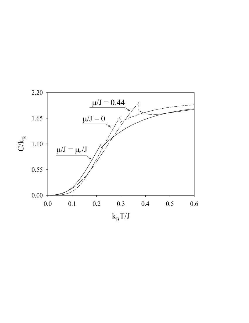
Figure 3: Specific heat vs. temperature $k_{B}T/J$ for $w/J=1$, $uJ=3$ and various values of chemical-potential, as indicated on the figure.

The temperature dependence of the specific is presented in Fig. 3. The low temperature behavior of $C(T)$ may be approximated by $C(T)\sim T^{3}$ for $\mu/J=0$ and $C(T)\sim T^{2.5}$ for $\mu/J=0.44$. For higher temperatures (but still below transition temperature) the linear behavior of the specific heat is observed. Reaching the critical temperature ($T_{c}$ or $T_{N}$), the specific heat experiences a finite jump (implying the value $\alpha=0$ for the critical exponent of the specific heat). For higher temperatures, saturation is observed.

IV Summary and final remarks

In conclusion, we have calculated entropy and specific heat dependence on temperature and various other parameters using the unified theory of antiferromagnetism and superconductivity proposed for the high-$T_{c}$ cuprates by Zhang and based on the SO(5) symmetry between antiferromagnetic and superconducting states. The theory of yields a qualitative scenario for the evolution of thermodynamic functions behavior, which is consistent with experiments. Most experimental work on the specific heat in the high-$T_{c}$ superconductors have concentrated on yttrium compound (Y-123). Junod1 ; Junod2 ; Junod3 Optimally doped Y-123 does not show a jump in the specific heat, but $\lambda$-peak at $T_{c}$. However, the shape for overdoped Y-123 is intermediate between a BCS step and a $\lambda$-type transition. Furthermore, optimally doped Bi-2212 shows a symmetric anomaly (intermediate between $\lambda$-peak and finite jump). Experimentally, the specific heat is not very sensitive to the critical exponent $\alpha$ and one can ascertain that $|\alpha|\ll 1$ for Y-123 compounds. However, the result of the present work ($\alpha=0$) agrees with the critical behavior of the 3D-XY model. Finally, checking the validity of basic principles of the SO(5) theory, by comparing parameters discussed here with relevant, obtained from calculations on microscopic models of high-$T_{c}$ superconductors is still called for.

References

• (1) S.C. Zhang, Science 275, 1089 (1997)
• (2) C. Henley, Phys. Rev. Lett. 80, 3590 (1998)
• (3) S. Rabello, H. Kohno, E. Demler, and S.C. Zhang, Phys. Rev. Lett. 80, 3568 (1998)
• (4) C. Burgess, J. Cline, R. MacKenzie, and R. Ray, Phys. Rev. B 57, 8549 (1998)
• (5) D. Scalapino, S.C. Zhang, and W. Hanke, Phys. Rev. B 58, 443 (1998)
• (6) R. Eder et al., Phys. Rev. B 59, 561 (1999)
• (7) E. Arrigoni and W. Hanke, Phys. Rev. Lett. 82, 21115 (1999)
• (8) S. Meixner, W. Hanke, E. Demler, and S.C. Zhang, Phys. Rev. Lett. 79, 4902 (1997)
• (9) T.A. Zaleski and T.K. KopeΔ‡, Phys. Rev. B 62, 9059 (2000)
• (10) T.K. KopeΔ‡ and T.A. Zaleski, Phys. Rev. Lett. 87, 097002 (2001)
• (11) T.A.Β Zaleski and T.K.Β KopeΔ‡, Phys. Rev. B 64, 144522 (2001)
• (12) Our approach is not restricted to the three dimensional cubic lattice and can be easily accommodated to virtually any other lattice (by using the proper density of states function).
• (13) M. Abramovitz and I. Stegun, Handbook of Mathematical Functions (Dover, New York, 1970).
• (14) T.H. Berlin and M. Kac, Phys. Rev. 86, 821 (1952); H.E. Stanley, ibid. 176, 718 (1968); G.S. Joyce, Phys. Rev. 146, 349 (1966); G.S. Joyce, in Phase Transitions and Critical Phenomena, edited by C. Domb and M.S. Green (Academic, New York, 1972), Vol. 2, p. 375.
• (15) J.W. Loram, et all., Physica C 341-348, 831 (2000)
• (16) M. Roulin, A. Junod, E. Walker, Physica C 260, 257 (1996)
• (17) M. Roulin, A. Junod, E. Walker, Physica C 296, 137 (1998)
• (18) A. Junod, et all., Physica B 280, 214 (2000)