Spin-chirality duality in a spin ladder with four-spin cyclic exchange

Abstract

Effect of four-spin cyclic exchange on magnetism is studied in the two-leg $S=1/2$ ladder. We develop an exact spin-chirality duality transformation, under which the system is self-dual when the four-spin exchange $J_{4}$ is half of the two-spin exchange. Using the density-matrix renormalization-group method and the duality relation, we find that the four-spin exchange makes the vector chirality correlation dominant. A “chirality short-range resonating-valence-bond” phase is identified for the first time at large $J_{4}$.

Recently, it has been realized that the two-leg $S=1/2$ ladder compound La_xCa_14-xCu₂₄O₄₁Brehmer ; Matsuda ; Schmidt ; Nunner and two-dimensional (2D) antiferromagnet La₂CuO₄HondaKW ; Coldea have a certain strength of four-spin cyclic exchange interactions. Theoretically, four-spin cyclic exchange emerges in the strong-coupling expansion of the one-band HubbardTakahashi and $d$-$p$SchmidtT models as the leading correction to the nearest-neighbor two-spin exchange. Cyclic exchanges were also found to be large in magnetism of 2D quantum solids, e.g. solid ³He filmsRoger and Wigner crystalsOkamoto . The effect of four-spin cyclic exchange on magnetism is, however, hardly understood, since it has frustration by itself: the question of what type of magnetic ordering tends to be realized by the four-spin exchange is still unsettled. For example, in the context of magnetism of solid ³He films, it was argued that the four-spin exchange on the triangular lattice can induce scalar chiralityKuboM , though finite-size system analysis could not find evidence for such ordering, instead showing spin-liquid ground statesMisguich .

To clarify magnetism induced by the four-spin cyclic exchange, we consider the spin ladder. Spin ladder antiferromagnets have been attracting extensive interest because they have a spin gap, a short-range resonating-valence-bond (RVB) ground state, and superconductivity upon dopingDagottoR . On the two-leg $S=1/2$ ladder it was shown numerically that the spin gap decreases rapidly with increasing the four-spin cyclic exchange $J_{4}$Brehmer and vanishes at a critical point, $J_{4}/J\simeq 0.3$ where $J$ is the two-spin exchange HondaH ; HijiiN . The nature of the new phase for large $J_{4}$ was not established.

In this letter, we show that the four-spin exchange in the two-leg $S=1/2$ ladder has a tendency to induce a vector chirality correlation. First, we describe an exact duality transformation between the Néel-spin operator $\left({\bf s}_{1,l}-{\bf s}_{2,l}\right)/2$ and the vector-chirality one ${\bf s}_{1,l}\times{\bf s}_{2,l}$ on the rungs, where ${\bf s}_{\mu,l}$ is the spin operator at the site on the leg $\mu=1,2$ and the rung $l$. The system is self-dual under this transformation at $J_{4}/J=1/2$, where the Néel-spin and the chirality interchange their roles: the former gives the most dominant correlation for small $J_{4}$ while the latter does for large $J_{4}$. Using the density-matrix renormalization-group (DMRG) methodWhite1 and the spin-chirality duality, we studied the ground-state phase diagram of the ladder for the whole region of $0\leq J_{4}\leq\infty$. We find the spin short-range RVB phase, an intermediate phase with a very small spin gap, and a novel chirality short-range RVB phase. Our findings of exotic magnetic states with dominant vector-chirality correlation at large $J_{4}$ suggest that the four-spin exchange can induce exotic electronic states in doped systems such as high-T_c superconductors, whereas only two-spin exchanges have been taken into account in $t$-$J$ models in searching the mechanism.

Let us consider the Hamiltonian defined as

$${\cal H} = \sum_{l}\{J_{\rm rung}{\bf s}_{1,l}\cdot{\bf s}_{2,l}+J_{\rm leg}({\bf s}_{1,l}\cdot{\bf s}_{1,l+1}$$ (1)

$$+{\bf s}_{2,l}\cdot{\bf s}_{2,l+1})+J_{4}K_{l}\},$$

where $J_{\rm rung}$ ($J_{\rm leg}$) denotes the two-spin exchange constant on rungs (legs) and $K_{l}$ the four-spin cyclic exchange on a plaquette $\{(1,l),(2,l),(2,l+1),(1,l+1)\}$,

$$K_{l} = {\bf s}_{1,l}\cdot{\bf s}_{2,l}+{\bf s}_{1,l+1}\cdot{\bf s}_{2,l+1}+{\bf s}_{1,l}\cdot{\bf s}_{1,l+1}$$ (2)

$$+ {\bf s}_{2,l}\cdot{\bf s}_{2,l+1}+{\bf s}_{1,l}\cdot{\bf s}_{2,l+1}+{\bf s}_{2,l}\cdot{\bf s}_{1,l+1}$$

$$+ 4({\bf s}_{1,l}\cdot{\bf s}_{2,l})({\bf s}_{1,l+1}\cdot{\bf s}_{2,l+1})$$

$$+ 4({\bf s}_{1,l}\cdot{\bf s}_{1,l+1})({\bf s}_{2,l}\cdot{\bf s}_{2,l+1})$$

$$- 4({\bf s}_{1,l}\cdot{\bf s}_{2,l+1})({\bf s}_{2,l}\cdot{\bf s}_{1,l+1}).$$

All the coupling constants are assumed to be positive, $J_{\rm rung},J_{\rm leg},J_{4}>0$. It is instructive to rewrite the Hamiltonian (1) as

$${\cal H} = (J_{\rm rung}+2J_{4})\sum_{l}{\bf s}_{1,l}\cdot{\bf s}_{2,l}$$ (3)

$$+ (J_{\rm leg}+J_{4})\sum_{l}\sum_{\mu=1,2}{\bf s}_{\mu,l}\cdot{\bf s}_{\mu,l+1}$$

$$+ J_{4}\sum_{l}\left({\bf s}_{1,l}\cdot{\bf s}_{2,l+1}+{\bf s}_{1,l+1}\cdot{\bf s}_{2,l}\right)$$

$$+ 4J_{4}\sum_{l}\left({\bf s}_{1,l}\cdot{\bf s}_{2,l}\right)\left({\bf s}_{1,l+1}\cdot{\bf s}_{2,l+1}\right)$$

$$+ 4J_{4}\sum_{l}\left({\bf s}_{1,l}\times{\bf s}_{2,l}\right)\cdot\left({\bf s}_{1,l+1}\times{\bf s}_{2,l+1}\right).$$

An interesting contribution of the cyclic exchange appears in the last term, which introduces a coupling between vector chiralities on nearest-neighbor rungs. This term tends to induce non-zero vector chiralities on every rung arranged in an antiparallel pattern. Hence, one can naively expect that for large $J_{4}$ the vector chirality becomes an important degree of freedom although the frustration between the various terms in eq. (3) complicates the situation. We will show later that the vector-chirality correlation indeed becomes dominant for large $J_{4}$.

To elucidate the relation between the spin and chirality degrees of freedom, we construct a duality transformation between them. Let us begin with the commutation relations between the total rung-spins ${\bf W}_{l}\equiv{\bf s}_{1,l}+{\bf s}_{2,l}$ and the vector chirality ${\bf V}_{l}\equiv 2~{}{\bf s}_{1,l}\times{\bf s}_{2,l}$ given by

$$\left[W^{\alpha}_{l},W^{\beta}_{l^{\prime}}\right] = i\epsilon^{\alpha\beta\gamma}W^{\gamma}_{l}\delta_{l,l^{\prime}},$$

$$\left[V^{\alpha}_{l},V^{\beta}_{l^{\prime}}\right] = i\epsilon^{\alpha\beta\gamma}W^{\gamma}_{l}\delta_{l,l^{\prime}},$$

$$\left[W^{\alpha}_{l},V^{\beta}_{l^{\prime}}\right] = i\epsilon^{\alpha\beta\gamma}V^{\gamma}_{l}\delta_{l,l^{\prime}}.$$

We note that the commutation relations are identical to those which hold between the angular momentum and the Runge-Lenz vector of an electron system in a hydrogen atom. We can disentangle the algebra by introducing new operators defined by

$${\bf S}_{l} \equiv \frac{1}{2}\left({\bf W}_{l}-{\bf V}_{l}\right)=\frac{1}{2}\left({\bf s}_{1,l}+{\bf s}_{2,l}\right)-{\bf s}_{1,l}\times{\bf s}_{2,l},$$ (4)

$${\bf T}_{l} \equiv \frac{1}{2}\left({\bf W}_{l}+{\bf V}_{l}\right)=\frac{1}{2}\left({\bf s}_{1,l}+{\bf s}_{2,l}\right)+{\bf s}_{1,l}\times{\bf s}_{2,l}.$$ (5)

These operators obey the commutation relations,

$$\left[S^{\alpha}_{l},S^{\beta}_{l^{\prime}}\right] = i\epsilon^{\alpha\beta\gamma}S^{\gamma}_{l}\delta_{l,l^{\prime}},$$

$$\left[T^{\alpha}_{l},T^{\beta}_{l^{\prime}}\right] = i\epsilon^{\alpha\beta\gamma}T^{\gamma}_{l}\delta_{l,l^{\prime}},$$

$$\left[S^{\alpha}_{l},T^{\beta}_{l^{\prime}}\right] = 0,$$

and satisfy ${\bf S}^{2}_{l}={\bf T}^{2}_{l}=3/4$. Thus, the new operators ${\bf S}_{l}$ and ${\bf T}_{l}$ are $S=1/2$ pseudo-spin operators decoupling each other. It is interesting to note that the original spins ${\bf s}_{1,l}$ and ${\bf s}_{2,l}$ may be expressed in terms of ${\bf S}_{l}$ and ${\bf T}_{l}$ simply by interchanging their roles in eqs. (4) and (5), i.e., ${\bf s}_{1,l}=\frac{1}{2}\left({\bf S}_{l}+{\bf T}_{l}\right)+{\bf S}_{l}\times{\bf T}_{l}$ and ${\bf s}_{2,l}=\frac{1}{2}\left({\bf S}_{l}+{\bf T}_{l}\right)-{\bf S}_{l}\times{\bf T}_{l}$. We hence call this a “duality” transformation. The relations between the original and new spin operators are summarized as

$${\bf s}_{1,l}+{\bf s}_{2,l} = {\bf S}_{l}+{\bf T}_{l},$$

$${\bf s}_{1,l}-{\bf s}_{2,l} = 2~{}{\bf S}_{l}\times{\bf T}_{l},$$

$$-2~{}{\bf s}_{1,l}\times{\bf s}_{2,l} = {\bf S}_{l}-{\bf T}_{l},$$

$${\bf s}_{1,l}\cdot{\bf s}_{2,l} = {\bf S}_{l}\cdot{\bf T}_{l}.$$

The transformation thereby exchanges the Néel-spin and the vector chirality on the same rung.

In terms of the new spin operators, the Hamiltonian (3) is rewritten as

$$\tilde{\cal H} = (J_{\rm rung}+2J_{4})\sum_{l}{\bf S}_{l}\cdot{\bf T}_{l}$$ (6)

$$+ \left(\frac{J_{\rm leg}}{2}+2J_{4}\right)\sum_{l}\left({\bf S}_{l}\cdot{\bf S}_{l+1}+{\bf T}_{l}\cdot{\bf T}_{l+1}\right)$$

$$+ \frac{J_{\rm leg}}{2}\sum_{l}\left({\bf S}_{l}\cdot{\bf T}_{l+1}+{\bf T}_{l}\cdot{\bf S}_{l+1}\right)$$

$$+ 4J_{4}\sum_{l}\left({\bf S}_{l}\cdot{\bf T}_{l}\right)\left({\bf S}_{l+1}\cdot{\bf T}_{l+1}\right)$$

$$+ 2J_{\rm leg}\sum_{l}\left({\bf S}_{l}\times{\bf T}_{l}\right)\cdot\left({\bf S}_{l+1}\times{\bf T}_{l+1}\right).$$

Thus, the duality transformation leaves the form of the Hamiltonian unchanged and only affects the coefficients of the second, third, and fifth terms. An interesting observation here is that in the case of $J_{4}=J_{\rm leg}/2$ the original Hamiltonian ${\cal H}$ and its dual $\tilde{\cal H}$ are equivalent including the coefficients. Hence the Néel-spin $\left({\bf s}_{1,l}-{\bf s}_{2,l}\right)/2$ and the vector chirality ${\bf s}_{1,l}\times{\bf s}_{2,l}$ show identical behavior on this “self-dual” line.

To clarify the consequence of the spin-chirality duality around $J_{4}=J_{\rm leg}/2$ and the nature of ground states, we study the low-energy properties of the Hamiltonian (3) numerically. For simplicity, we focus on the case of $J_{\rm rung}=J_{\rm leg}=J$ and investigate the ground-state phase diagram on the $J_{4}/J$ line hereafter. Using the DMRG methodWhite1 , we have calculated the energy gap of spin excitations

$$\Delta_{0M}(L)=E_{0}(L;M)-E_{0}(L;0),~{}~{}~{}~{}(M=1,2),$$ (7)

where $E_{0}(L;M)$ is the lowest energy in the subspace of $s^{z}_{\rm total}=\sum_{l}(s^{z}_{1,l}+s^{z}_{2,l})=M$ in a finite ladder of $L$ rungs. For the best performance of the DMRG method, an open boundary condition was imposed. We have also calculated the ground-state spin correlation functions

$$C^{s}_{0}(r) = \frac{1}{4}\langle\left(s^{z}_{1,l}+s^{z}_{2,l}\right)\left(s^{z}_{1,l^{\prime}}+s^{z}_{2,l^{\prime}}\right)\rangle,$$ (8)

$$C^{s}_{\pi}(r) = \frac{1}{4}\langle\left(s^{z}_{1,l}-s^{z}_{2,l}\right)\left(s^{z}_{1,l^{\prime}}-s^{z}_{2,l^{\prime}}\right)\rangle,$$ (9)

and the vector-chirality correlation function

$$C^{\kappa}(r)=\langle\left({\bf s}_{1,l}\times{\bf s}_{2,l}\right)^{z}\left({\bf s}_{1,l^{\prime}}\times{\bf s}_{2,l^{\prime}}\right)^{z}\rangle,$$ (10)

with $l=l_{0}-r/2$ and $l^{\prime}=l_{0}+r/2$Stot . The index $l_{0}$ represents the center position of the open ladder, i.e., $l_{0}=L/2$ for even $r$ and $l_{0}=(L+1)/2$ for odd $r$. We have employed the finite-system method with improved algorithmWhite1 and kept up to $m=500$ states per block. The numerical errors due to the truncation are estimated from the difference between the data of different $m$’s. The system size is up to $2\times 100$ sites.

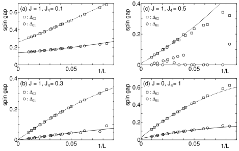
Figure 1: System-size dependence of the spin gaps for (a) $(J,J_{4})=(1,0.1)$; (b) $(1,0.3)$; (c) $(1,0.5)$; and (d) $(0,1)$. The gaps $\Delta_{01}(L)$ and $\Delta_{02}(L)$ are plotted by circles and squares, respectively. The numerical errors of the DMRG calculation are smaller than the symbols.

First, we discuss the parameter region $J_{4}/J<1$. It is known that for $J_{4}=0$ the system belongs to a spin-liquid phase, in which the ground state is well described by the RVB state. The spin gap is open in this phase. We show in Fig. 1 our numerical results for the spin gaps $\Delta_{0M}(L)$. The data are extrapolated by fitting them to a polynomial form, $\Delta_{0M}(L)=\Delta_{0M}(\infty)+a/L+b/L^{2}$. For $J_{4}/J\lesssim 0.3$, the spin gaps decrease smoothly for both $M$’s as $L$ increases, and consequently, the extrapolation works pretty well [see Fig. 1(a) and (b)]. The extrapolated values $\Delta_{0M}(\infty)$ are shown in Fig. 2 with $J=1$ in the region $J_{4}/J<1$. The spin gaps decrease smoothly as $J_{4}$ increases from $0$ and vanish around $J_{4}/J\simeq 0.3$, suggesting a phase transition accompanied by vanishing of the spin gap at $J_{4}/J=(J_{4}/J)_{\rm c1}\simeq 0.3$. Unfortunately, accurate estimation of the critical value $(J_{4}/J)_{\rm c1}$ is quite difficult due to the very slow vanishing of the spin gaps around the transition point. When $J_{4}/J$ is larger than $0.3$, $\Delta_{01}(L)$ shows bumpy behavior as seen in Fig. 1(c). This may be attributed to effects of open boundaries. The value of $\Delta_{01}(L)$ becomes exactly $0$ within numerical accuracy for several $L$, which suggests a spin-triplet ground state. On the other hand, the spin gap $\Delta_{02}(L)$ exhibits a rather smooth $L$-dependence even for $J_{4}/J\geq 0.3$. The extrapolated gaps $\Delta_{02}(\infty)$ are very small, less than $0.02$, but seem to be finite for this region. Very recently, Läuchli et al. studied independently the same model but with a different boundary condition and showed that the system for this parameter region belongs to a phase with a very small gap exhibiting the translational symmetry breakingLauchli . The work of Ref. Muller, also pointed toward this result. Our results are thus consistent with theirs although the number and type of excitations in the finite systems might differ from each other because of the different boundary conditions. Further studies, especially by analytic methods, are desirable for clarifying the nature of excitations and why the spin gap is so small in the entire region of the phase.

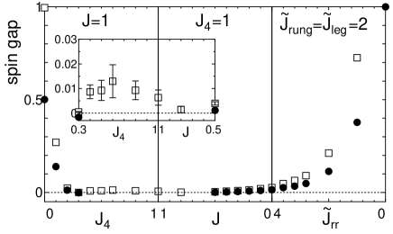
Figure 2: Extrapolated spin gaps in the limit $L\to\infty$ as functions of $J_{4}$ (left), $J$ (center), and $\tilde{J}_{\rm rr}$ (right); see text. The circles and squares represent $\Delta_{01}(\infty)$ and $\Delta_{02}(\infty)$, respectively. Inset: Enlarged figure for $0.3\leq J_{4}/J\leq 2$. The error bars represent those from the extrapolation procedure.

Figure 3 shows the spin correlations $C^{s}_{0}(r)$ and $C^{s}_{\pi}(r)$, and the vector-chirality correlation $C^{\kappa}(r)$ for several typical sets of parameters. For $J_{4}/J<(J_{4}/J)_{\rm c1}\simeq 0.3$, all the correlations decay exponentially, which is consistent with a finite spin gap. The Néel-spin correlation $C^{s}_{\pi}(r)$ is the strongest among the calculated correlation functions [Fig. 3(a)], as in the usual antiferromagnetic (AF) ladder. For $J_{4}/J>(J_{4}/J)_{\rm c1}$, on the other hand, the correlation functions decay very slowly reflecting the small spin gapopen . We find that the Néel-spin correlation $C^{s}_{\pi}(r)$, which is dominant for small $J_{4}$, keeps reducing as $J_{4}$ increases while the vector-chirality correlation $C^{\kappa}(r)$ keeps growing and becomes dominant for large $J_{4}$. They interchange with each other at the self-dual point $J_{4}/J=0.5$; we can see their perfect coincidence in Fig. 3(c). These results strongly suggest that the system exhibits symmetric behaviors with respect to the self-dual point $J_{4}/J=0.5$ with exchanging the roles of the Néel-spin and the vector-chirality correlations. We also note that the dimer operator $\vec{s}_{1,l}\cdot\vec{s}_{1,l+1}-\vec{s}_{2,l}\cdot\vec{s}_{2,l+1}$ and the scalar-chirality operator $(\vec{s}_{1,l}+\vec{s}_{2,l})\cdot(\vec{s}_{1,l+1}\times\vec{s}_{2,l+1})+(\vec{s}_{1,l}\times\vec{s}_{2,l})\cdot(\vec{s}_{1,l+1}+\vec{s}_{2,l+1})$ are related to each other by the duality transformation, and consequently, their correlation functions must interchange exactly at $J_{4}/J=0.5$, which is consistent with numerical results in Ref. Lauchli, .

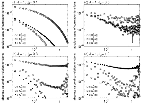
Figure 3: Correlation functions $|C^{s}_{\pi}(r)|$ (circles), $|C^{s}_{0}(r)|$ (squares), and $|C^{\kappa}(r)|$ (triangles) as functions of distance for $J=1$ and (a) $J_{4}=0.1$; (b) $J_{4}=0.3$; (c) $J_{4}=0.5$; and (d) $J_{4}=1$. The system size is $L=80$. The error bars represent the numerical errors of the DMRG calculation.

Next, we consider the parameter region $J_{4}/J>1$. Hereafter, we set $J_{4}=1$. It can be seen in Fig. 2 that the spin gaps open for $J_{4}/J>(J_{4}/J)_{\rm c2}\simeq 1/0.4=2.5$. Again, accurate estimation of $(J_{4}/J)_{\rm c2}$ is quite difficult due to the very slow opening of the gaps. We also note that for large $J_{4}/J$ the spin gap $\Delta_{01}$ exhibits a smooth $L$-dependence and does not become $0$ for finite $L$ [see Fig. 1(d)], suggesting the absence of the triplet ground state in the finite systems. To elucidate the nature of the system in this large $J_{4}/J$ region, we consider the case $J_{4}/J=\infty$ ($J_{4}=1$ and $J=0$) using the spin-chirality duality transformation. In this case, the transformed Hamiltonian (6) is expressed as

$$\tilde{\cal H}_{J_{4}} = \tilde{J}_{\rm rung}\sum_{l}{\bf S}_{l}\cdot{\bf T}_{l}+\tilde{J}_{\rm leg}\sum_{l}\left({\bf S}_{l}\cdot{\bf S}_{l+1}+{\bf T}_{l}\cdot{\bf T}_{l+1}\right)$$ (11)

$$+ \tilde{J}_{\rm rr}\sum_{l}\left({\bf S}_{l}\cdot{\bf T}_{l}\right)\left({\bf S}_{l+1}\cdot{\bf T}_{l+1}\right)$$

with $\tilde{J}_{\rm rung}=\tilde{J}_{\rm leg}=2$ and $\tilde{J}_{\rm rr}=4$. Notice here that, if one sets $\tilde{J}_{\rm rr}=0$ in eq. (11), the system is equivalent to the usual two-leg AF ladder, which has the short-range RVB ground state consisting of the spins ${\bf S}_{l}$ and ${\bf T}_{l}$. In Fig. 2, we show the $\tilde{J}_{\rm rr}$-dependence of the extrapolated spin gaps $\Delta_{0M}(\infty)$ for $0\leq\tilde{J}_{\rm rr}\leq 4$. It is clear that the spin gaps remain finite for the entire region of $0\leq\tilde{J}_{\rm rr}\leq 4$ and are smoothly connected to the spin gaps at $\tilde{J}_{\rm rr}=4$; there is no phase transition between $\tilde{J}_{\rm rr}=0$ and $\tilde{J}_{\rm rr}=4$. We thus conclude that the Hamiltonian (11) with $\tilde{J}_{\rm rr}=4$, and accordingly, the original ladder (3) in the limit $J_{4}/J=\infty$ belong to the same RVB phase as the AF ladder of the spins ${\bf S}_{l}$ and ${\bf T}_{l}$ with $\tilde{J}_{\rm rr}=0$. Small size of the spin gap at $J_{4}/J=\infty$ can be understood from the fact that the system is close to the quantum critical point between the short-range RVB and intermediate phases. Note that the dominant correlation function in this RVB phase is that of the Néel-spin $\left({\bf S}_{l}-{\bf T}_{l}\right)/2$ and hence, in terms of the original spins, the correlation of the vector chirality ${\bf s}_{1,l}\times{\bf s}_{2,l}$ is the strongest. We therefore term this novel phase the chirality short-range RVB phase.

To summarize, using the spin-chirality duality transformation, which is developed in this letter, as well as the DMRG method, we have found that the four-spin cyclic exchange makes the vector chirality correlation dominant. The chirality RVB phase appears for large $J_{4}$. It has been found that the system exhibits symmetric behavior with respect to the self-dual point $J_{4}/J=1/2$ by interchanging the Néel spin and the vector chirality. We remark that the duality transformation is applicable to any spin Hamiltonian, since it is based only on the spin commutation relation. This transformation should be useful in studying various topics. One example is the spin-orbital model around the SU(4) symmetric pointYamashita . We have found in the two-leg ladder with extended four-spin exchange that the self-dual line connects with the SU(4)-symmetric pointHikiharaMH2 . Another example is a magnetization plateau induced by the four-spin exchangeSakai . Since the total spin $\sum_{\mu,l}{\bf s}_{\mu,l}$ is invariant under the dual transformation, the duality relation holds even in a magnetic field. Effect of four-spin exchange on hole-doped systems is also to be considered. It would be interesting to investigate relation to possible hidden orders proposed for high-T_c superconductors, e.g. the staggered currents.

We would like to thank K. Kubo, N. Taniguchi, A. Tanaka, K. Nomura and M. Nakamura for stimulating discussions. We also thank A. Läuchli for useful comments. T.M. was supported by Monkashou (MEXT) in Japan through Grant Nos. 13740201 and 1540362.

References

(1) S. Brehmer et al.,
Phys. Rev. B 60, 329 (1999).
(2) M. Matsuda et al.,
Phys. Rev. B 62, 8903 (2000); J. Appl. Phys. 87,
6271 (2000).
(3) K. P. Schmidt et al.,
Europhys. Lett. 56, 877 (2001).
(4) T. S. Nunner et al., cond-mat/0203472.
(5) Y. Honda et al.,
Phys. Rev. B 47, 11329 (1993).
(6) R. Coldea et al.,
Phys. Rev. Lett. 86, 5377 (2001).
(7)
M. Takahashi, J. Phys. C: Solid State Phys. 10, 1289
(1977).
(8)
H. J. Schmidt and Y. Kuramoto, Physica C 167, 263 (1990).
(9) M. Roger, et al., Phys. Rev. Lett. 80,
1308 (1998).
(10) T. Okamoto and S. Kawaji, Phys. Rev. B 57,
9097 (1998).
(11)
K. Kubo and T. Momoi, Z. Phys. B. 103, 485 (1997);
T. Momoi et al.,
Phys. Rev. Lett. 79, 2081 (1997).
(12) G. Misguich et al.,
Phys. Rev. Lett. 81, 1098 (1998);
Phys. Rev. B 60, 1064 (1999).
(13) E. Dagotto and T. M. Rice,
Science 271, 618 (1996) and references therein.
(14) Y. Honda and T. Horiguchi, preprint, cond-mat/0106426.
(15) K. Hijii and K. Nomura, Phys. Rev. B
65 104413, (2002).
(16)
S. R. White, Phys. Rev. Lett. 69, 2863 (1992); Phys. Rev. Lett. 77, 3633 (1996).
(17)
To be precise, the correlation functions are calculated in the
lowest-energy state in the subspace , which
must be the ground state or, at least, one of the ground states
since the Hamiltonian is symmetric.
(18) A. Läuchli et al., preprint, cond-mat/0206153.
(19)
M. Müller et al., preprint, cond-mat/0206081.
(20)
We note that the enhancement of the correlations seen for large is due to the presence of the open boundaries and is not
essential.
(21) Y. Yamashita et al.,
Phys. Rev. B 58, 9114 (1998).
(22) T. Momoi et al.,
in preparation.
(23)
A. Nakasu, et al., J. Phys.: Condens. Matter, 13,
7421 (2001).