Dynamical symmetries in Kondo tunneling through complex quantum dots

Abstract

Kondo tunneling reveals hidden $SO(n)$ dynamical symmetries of evenly occupied quantum dots. As is exemplified for an experimentally realizable triple quantum dot in parallel geometry, the possible values $n=3,4,5,7$ can be easily tuned by gate voltages. Following construction of the corresponding $o_{n}$ algebras, scaling equations are derived and Kondo temperatures are calculated. The symmetry group for a magnetic field induced anisotropic Kondo tunneling is $SU(2)$ or $SO(4)$.

While theoretical predictions of the Kondo effect in tunneling through quantum dots (QD) under strong Coulomb blockade conditions Glaz have been confirmed Gogo , it should be born in mind that representing a real nanoobject by a single localized spin S=1/2 is inadequate. Ubiquitous low-lying spin excitations in few-electron systems cannot be ignored. Even in ”classical” planar QDs formed in GaAs/GaAlAs heterostructures the Kondo physics is much richer than that employed in analyzing the seminal experiments Gogo .

The purpose of the present work is to demonstrate that if low-lying spin excitations are properly incorporated, the exchange Hamiltonian of quantum dots with even occupation ${\cal N}$ unveils an unusual dynamical $SO(n)$ symmetry, and to suggest experiments for its elucidation. Analysis of relatively simple QD systems indicates the possible emergence of higher symmetries. For example, Kondo tunneling may be induced by external magnetic field in planar QD Misha , since occurrence of low-lying triplet exciton above singlet ground state leads to an $SO(4)$ symmetry. Due to Zeeman splitting, it is reduced to $SU(2)$, leading to the Kondo effect in strong magnetic field. Similar scenario may be realized in vertical QDs Eto where now the Larmor (instead of the Zeeman) effect comes into play. Another example is a double quantum dot with ${\cal N}=2$ which is a spin analog of a hydrogen molecule ${\rm H_{2}}$. Here, the low lying singlet/triplet manifold possesses the symmetry $SO(4)$ of a ”spin rotator” KA01 ; KA02 .

The central (and fundamental) question is then: Is the physics of Kondo tunneling through complex quantum dots intimately related with hidden $SO(n)$ symmetries? The answer given below is affirmative. Moreover, these symmetries can be experimentally realized and the specific value of $n$ can be controlled by gate voltage and/or tunneling strength. To be concrete, the analysis is carried out below for a triple quantum dot (TQD) in a parallel geometry with ${\cal N}=4$ as a neutral ground state (see Fig. 1). It is shown to exhibit an $SO(n)$ symmetry, and the relations of tunneling strengths $V_{l,r}$ and gate voltages $V_{gl},V_{gr}$ with the possible values $n=3,4,5,7$ and the corresponding Kondo temperatures are explicitly demonstrated. This example is simple enough to allow the construction of the corresponding $o_{n}$ algebras and solving the poor-man scaling equations for obtaining the Kondo temperatures. At the same time, it paves the way for treating more general QD structures with arbitrary scheme of low lying spin excitations.

Initially, the TQD in Fig. 1 is treated within an Anderson-type model with bare level operators $d_{\sigma i}$, energies $\varepsilon_{i}$, charging energies $Q_{i}$ and gate voltages $V_{gi}$ with $i=l,c,r$ for left, center and right dots. The figure also defines inter-dot hopping ($W_{a}$) and tunneling matrix elements ($V_{a}$) where the notation $a=l,r$ and ${\bar{a}}=r,l$ is used ubiquitously hereafter. It is useful to shift the energies as $\epsilon_{i}=\varepsilon_{i}-V_{gi}$ which can be experimentally manipulated. Setting the Fermi energy in the leads to be $\varepsilon_{F}=0$, the pertinent “Kondo limit” is determined as, $0>\epsilon_{a}\gg\epsilon_{c}$ and $0<\epsilon_{a}+Q_{a}\ll\epsilon_{c}+Q_{c}$ KA01 . The capacitive interaction between the three dots is tuned in such a way that, in the absence of inter-dot hopping, the neutral ground state has the occupation, $n_{a}=2,n_{c}=n_{\bar{a}}=1$ while 5 electron states cost much energy and are discarded.

Figure 1: Triple quantum dot in parallel geometry.

Next, the isolated dot Hamiltonian is diagonalized in the Hilbert space which is a direct sum of 3 and 4 electron states, $|\lambda\rangle$ and $|\Lambda\rangle$, using Hubbard operators $X^{\gamma\gamma}=|\gamma\rangle\langle\gamma|$ ($\gamma=\lambda,\Lambda$) Hew . The four particle states $|\Lambda\rangle=(|\Lambda_{l}\rangle,|\Lambda_{r}\rangle)$ exhaust the lowest part of the spectrum, an octet consisting of two singlets $|S_{l}\rangle,|S_{r}\rangle$, and two triplets $|T_{l}\rangle,|T_{r}\rangle$. Just above it, there is a charge transfer exciton $|ex\rangle$. The corresponding energies are,

$$E_{S_{a}} = {\epsilon}_{c}+{\epsilon}_{a}+2{\epsilon}_{\bar{a}}+Q_{\bar{a}}-2W_{a}\beta_{a},$$

$$E_{{T_{a}}} = {\epsilon}_{c}+{\epsilon}_{a}+2{\epsilon}_{\bar{a}}+Q_{\bar{a}},$$

$$E_{ex} = 2{\epsilon}_{l}+2{\epsilon}_{r}+Q_{l}+Q_{r}+2W_{l}\beta_{l}+2W_{r}\beta_{r}.$$ (1)

where $\beta_{a}=W_{a}/\Delta_{a}\ll 1$ $(\Delta_{a}=Q_{a}+\epsilon_{a}-\epsilon_{c})$. Finally, tunneling operators in the bare Anderson Hamiltonian are replaced by a product of number changing Hubbard operators $X^{\lambda\Lambda}$ and a combination $c_{k\sigma}=2^{-1/2}(c_{k\sigma s}+c_{k\sigma d})$ of lead electron operators, ($k=$momentum, $\sigma=$ spin projection and $s,d$ stand for source and drain).

With these preliminaries, the starting point is a generalized Anderson Hamiltonian describing the TQD in tunneling contact with the leads,

$$H_{A} = \sum_{k\sigma b=s,d}\epsilon_{kb}c^{\dagger}_{k\sigma b}c_{k\sigma b}+\sum_{\gamma=\Lambda\lambda}{E}_{\gamma}X^{\gamma\gamma}$$ (2)

$$+ \left(\sum_{\Lambda\lambda}\sum_{k\sigma a}V^{\Lambda\lambda}_{\sigma a}c^{\dagger}_{k\sigma}X^{\lambda\Lambda}+h.c.\right),$$

with dispersion $\epsilon_{kb}$ of electrons in the leads and $V^{\lambda\Lambda}_{\sigma a}\equiv V_{a}\langle\lambda|d_{\sigma a}|\Lambda\rangle$. The Kondo effect at $T>T_{K}$ is unraveled by employing a renormalization group (RG) procedure Hew ; Hald in which the energies $E_{\gamma}$ are renormalized as a result of rescaling high-energy charge excitations. Our attention, though, is focused on renormalization of $E_{S_{a}},E_{T_{a}}$ (1). Since the deep central level $\epsilon_{c}$ as well as the tunnel constants are irrelevant variables KA01 ; Hald , the scaling equations are

$$\pi\,dE_{\Lambda}/d\ln D=\Gamma_{\Lambda}.$$ (3)

Here $2D$ is the conduction electron bandwidth, $\Gamma_{\Lambda}$ are the tunneling strengths,

$$\Gamma_{T_{a}}=\pi\rho_{0}\left(V_{a}^{2}+2V_{\bar{a}}^{2}\right),\;\;\Gamma_{S_{a}}=\alpha_{a}^{2}\Gamma_{T_{a}},$$ (4)

with $\alpha_{a}=\sqrt{1-2\beta_{a}^{2}}$ and $\rho_{0}$ being the density of states at $\varepsilon_{F}$. The scaling invariants for equations (3),

$$E_{\Lambda}^{\ast}=E_{\Lambda}(D)-\pi^{-1}\Gamma_{\Lambda}\ln(\pi D/\Gamma_{\Lambda}),$$ (5)

are tuned to satisfy the initial condition $E_{\Lambda}(D_{0})=E_{\Lambda}^{(0)}$. Equations (3) determine four scaling trajectories $E_{\Lambda}(D)$ for two singlet and two triplet states. Note that the level $E_{ex}$ is irrelevant, but admixture of the bare exciton ($n_{a}=n_{\bar{a}}=2$) in the singlet states is crucial for the inequality of tunneling rates $\Gamma_{T_{a}}>\Gamma_{S_{a}}$ (cf. KA01 ; KA02 ). As a result, the energies $E_{T_{a}}(D)$ decrease with $D$ faster than $E_{S_{a}}(D)$, so that the trajectories $E_{T_{a}}(D,\Gamma_{T_{a}})$ intersect $E_{S_{a}}(D,\Gamma_{S_{a}})$ at certain points $D^{(a)}=D^{(a)}_{c}$. This level crossing may occur either before or after reaching the Schrieffer-Wolff (SW) limit where $E_{\Lambda}(D)\sim D$ and scaling terminates Hald . Hidden dynamical symmetries affect the Kondo tunneling most effectively when the scaling trajectories cross near the SW boundary $E_{\Lambda}(D_{c})\sim D_{c}$. An example of this scenario is shown in Fig. 2. As a result, various patterns of occasional degeneracy may arise depending on the initial conditions (1), which, in turn, determine the pertinent $SO(n)$ symmetry of the resulting spin excitations (see below).

The above Haldane RG procedure brings us to the SW limit SW , where all charge degrees of freedom are quenched. By properly tuning the SW transformation $e^{iS}$ the effective Hamiltonian $H=e^{iS}H_{A}e^{-iS}$ is of the $s-d$ type Hew . However, unlike the conventional case SW of doublet spin 1/2 we have here an octet $\Lambda=\{\Lambda_{l},\Lambda_{r}\}=\{S_{l},T_{l},S_{r},T_{r}\}$, and the SW transformation intermixes all these states. To order $O(|V|^{2})$, then,

$$H=\sum_{\Lambda,a}E_{\Lambda_{a}}X^{\Lambda_{a}\Lambda_{a}}+\sum_{a}J^{T}_{a}{\bf S}_{a}\cdot{\bf s}+J_{lr}{\hat{P}}\sum_{a}{\bf S}_{a}\cdot{\bf s}$$

$$+\sum_{a}J^{ST}_{a}{\bf M}_{a}\cdot{\bf s}+J_{lr}\sum_{a}{\bf B}_{a}\cdot{\bf s}+\sum_{k\sigma b}\epsilon_{kb}c^{\dagger}_{k\sigma b}c_{k\sigma b}.$$ (6)

The vector operators, ${\bf S}_{a},{\bf M}_{a},{\bf B}_{a}$ and the permutation operator ${\hat{P}}$ manifest the dynamical symmetry of TQD. Their spherical components are defined via Hubbard operators connecting different states of the octet:

$$S^{+}_{a} = \sqrt{2}(X^{1_{a}0_{a}}+X^{0_{a}\bar{1}_{a}}),\ \ S^{-}_{a}=(S^{+}_{a})^{\dagger},$$

$$S^{z}_{a} = X^{1_{a}1_{a}}-X^{\bar{1}_{a}\bar{1}_{a}},$$

$$M^{+}_{a} = \sqrt{2}(X^{1_{a}S_{a}}-X^{S_{a}\bar{1}_{a}}),\ \ M^{-}_{a}=(M^{+}_{a})^{\dagger},$$

$$M^{z}_{a} = -(X^{0_{a}S_{a}}+X^{S_{a}0_{a}}),$$

$$B^{+}_{a} = \sqrt{2}(\alpha_{\bar{a}}X^{1_{a}S_{\bar{a}}}-\alpha_{a}X^{S_{a}\bar{1}_{\bar{a}}}),\ \ B^{-}_{a}=(B^{+}_{\bar{a}})^{\dagger},$$

$$B^{z}_{a} = -(\alpha_{\bar{a}}X^{0_{a}S_{\bar{a}}}+\alpha_{a}X^{S_{a}0_{\bar{a}}}).$$ (7)

Here ${\bf S}_{a}$ are spin 1 operators with projections ${\mu}_{a}=1_{a},0_{a},{\bar{1}_{a}}$, while ${\bf M}_{a}$ and ${\bf B}_{a}$ couple singlet $|S_{a}\rangle$ with triplet $\langle T_{a}\mu_{a}|$ and $\langle T_{\bar{a}}\mu_{\bar{a}}|$ respectively. The permutation ${\hat{P}}\equiv\sum_{a}(X^{S_{a}S_{\bar{a}}}+\sum_{\mu}X^{\mu_{a}\mu_{\bar{a}}})$ commutes with ${\bf S}_{l}+{\bf S}_{r}$ and ${\bf M}_{l}+{\bf M}_{r}$, while ${\bf s}=\frac{1}{2}\sum_{kk^{\prime}}\sum_{\sigma\sigma^{\prime}}c^{\dagger}_{k^{\prime}{\sigma}^{\prime}}\hat{\tau}_{\sigma\sigma^{\prime}}c_{k\sigma},$ with Pauli matrices $\hat{\tau}$ is the conduction electron spin operator. Finally, the (antiferromagnetic) coupling constants are $J^{T}_{a}=2V_{a}^{2}/\Delta_{a},\;J^{ST}_{a}=\alpha_{a}J^{T}_{a},\;J_{lr}=V_{l}V_{r}\sum_{a}\Delta_{a}^{-1}$  $(\Delta_{a}=\varepsilon_{F}-\epsilon_{a})$.

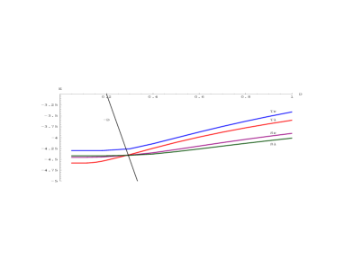
Figure 2: Scaling trajectories resulting in an $SO(5)$ symmetry in the SW regime.

After arriving at the $s-d$ Hamiltonian (6) the last stage implies the solution of Anderson poor-man scaling equations Anders for extracting the corresponding Kondo temperatures. The discussion below exhausts all possible realizations of $SO(n)$ symmetries arising in TQD.

The most symmetric case is realized when ${\Delta_{l}}={\Delta_{r}}$ and ${\Gamma_{T_{r}}}={\Gamma_{T_{l}}}$. If all four phase trajectories $E_{\Lambda}(D)$ intersect at $D=D_{c}$, the symmetry of the TQD is $\hat{P}\times SO(4)\times SO(4)$. The operator $\bf B$ transforms into $\hat{P}{\bf M}$, and the exchange part of $H$ (6) reduces to

$$H_{int}=J^{T}\sum_{a}(1+{\hat{P}}){\bf S}_{a}\cdot{\bf s}+J^{ST}\sum_{a}(1+{\hat{P}}){\bf M}_{a}\cdot{\bf s}.$$ (8)

The vector operators ${\bf M_{a}}$ and ${\bf S_{a}}$ obey the commutation relations of $o_{4}$ Lie algebra,

$$[S_{aj},S_{ak}]=ie_{jkm}S_{am},\;\;[M_{aj},M_{ak}]=ie_{jkm}S_{am},$$

$$[M_{aj},S_{ak}]=ie_{jkm}M_{am}.$$ (9)

(here $j,k,m$ are Cartesian indices). Besides, ${\bf S}_{a}\cdot{\bf M}_{a}=0,$ and the Casimir operator is ${\bf S}_{a}^{2}+{\bf M}_{a}^{2}=3.$ This justifies the qualification of such TQD as a double spin rotator. Scaling equations for $J_{T}$ and $J_{ST}$ are,

$$\frac{dj_{1}}{d\ln d}=-2\left[(j_{1})^{2}+(j_{2})^{2}\right],~{}~{}\frac{dj_{2}}{d\ln d}=-4j_{1}j_{2},$$ (10)

with $j_{1}=\rho_{0}J^{T},j_{2}=\rho_{0}J^{ST},d=\rho_{0}D$. In the limit of complete degeneracy the system (10) is reduced to a single equation, $dj_{+}/d\ln d=-2(j_{+})^{2}$ for $j_{+}=j_{1}+j_{2}$. Its solution yields the Kondo temperature $T_{K0}=\bar{D}\exp(-1/2j_{+}),$ which is an obvious generalization of that derived for a QD with $SO(4)$ symmetry and triplet ground state Eto ; KA01 ; KA02 . The net spin of the TQD is also $S=1$, and the residual under-screened spin is $\tilde{S}=1/2$. If the occasional S/T symmetry is lifted, $\bar{\delta}=E_{S}(D_{c})-E_{T}(D_{c})>0$, but the TQD still conserves its permutation symmetry, the Kondo temperature is not universal anymore, since the scaling of $j_{2}$ terminates at $D\approx\bar{\delta}$ (cf. Eto ). Analytic solution of Eqs. (10) obtains when $|\bar{\delta}|\gg T_{K0}$, for which $j_{2}\approx\alpha j_{1}$ and $T_{K}/T_{K0}\approx(T_{K0}/\bar{\delta})^{\alpha}.$ The symmetry of TQD in this case is ${\hat{P}}\times SO(3)\times SO(3)$.

For the symmetric configurations considered so far, the properties of TQD are similar to those of DQD, supplemented by the permutation operation. Much richer are asymmetric configurations where ${\Delta_{l}}\neq{\Delta_{r}}$, ${\Gamma_{T_{l}}}\neq{\Gamma_{T_{r}}}$. When ${\bar{E}}_{S_{l}}\approx{\bar{E}}_{T_{l}}\approx{\bar{E}}_{S_{r}}<{\bar{E}}_{T_{r}}$ (Fig. 2), the TQD possesses an $SO(5)$ symmetry. The group generators of the $o_{5}$ algebra are the ”left” vectors ${\bf S}_{l},{\bf M}_{l}$ and the vector ${\bf B}$ (with $B^{+}=\sqrt{2}(X^{1_{l}S_{r}}-X^{S_{r}{\bar{1}}_{l}}),$ $B^{-}=(B^{+})^{\dagger},$ $B_{z}=-(X^{0_{l}S_{r}}+X^{S_{r}0_{l}})),$ supplemented by the scalar operator $\hat{T}=i(X^{S_{r}S_{l}}-X^{S_{l}S_{r}})$. Thus,

$$[S_{lj},S_{lk}]=ie_{jkm}S_{lm},\;\;\;\;[M_{lj},M_{lk}]=ie_{jkm}S_{lm},$$

$$[B_{j},S_{lk}]=ie_{jkm}B_{m},\;\;\;\;\;[B_{j},B_{k}]=ie_{jkm}S_{lm},$$

$$[M_{lj},S_{lk}]=ie_{jkm}M_{lm},\;\;[M_{lj},B_{k}]=i{\hat{T}}{\delta}_{jk},$$

$$[B_{j},{\hat{T}}]=iM_{lj},\;\;\;[{\hat{T}},M_{lj}]=iB_{j},\;\;\;[{\hat{T}},S_{lj}]=0.$$ (11)

with ${\bf M}_{l}\cdot{\bf S}_{l}={\bf B}\cdot{\bf S}_{l}=0,$ ${\bf M}_{l}\cdot{\bf B}=3X^{S_{l}S_{r}},$ and Casimir operator ${\bf S}_{l}^{2}+{\bf M}_{l}^{2}+{\bf B}^{2}+T^{2}=4.$ The exchange Hamiltonian now reads,

$${H}_{int}=J_{1l}^{T}{\bf S}_{l}\cdot{{\bf s}}+J_{1l}^{ST}{\bf M}_{l}\cdot{{\bf s}}+\alpha_{r}J_{lr}{\bf B}\cdot{{\bf s}},$$ (12)

and the scaling equations are,

$$dj_{1}/d\ln d = -[j_{1}^{2}+j_{2}^{2}+j^{2}_{3}],$$

$$dj_{2}/d\ln d = -2j_{1}j_{2},\;\;dj_{3}/d\ln d=-2j_{1}j_{3},$$ (13)

where $j_{1}=\rho_{0}J^{T}_{1l}$, $j_{2}=\rho_{0}J^{ST}_{1l}$ and $j_{3}=\rho_{0}\alpha_{r}J_{lr}$. From Eqs.(13) the Kondo temperature is found,

$$T_{K1}=\bar{D}\exp\left\{-\left[j_{1}+\sqrt{j_{2}^{2}+j_{3}^{2}}\right]^{-1}\right\}.$$ (14)

Upon increasing $\bar{\delta}_{rl}=E_{S_{r}}({\bar{D}})-E_{T_{l}}({\bar{D}})$ the energy $E_{S_{r}}$ is quenched, and at ${\bar{\delta}}_{r}\gg T_{K1}$ the symmetry reduces to $SO(4)$, with Kondo temperature, $T_{K}=|{\bar{\delta}}_{r}|\exp\{-[j_{1}(|{\bar{\delta}}_{r}|)+j_{2}({\bar{\delta}}_{r})]^{-1}\}$ (cf. KA02 ). On the other hand, upon decreasing $\bar{\delta}_{r}=E_{T_{r}}({\bar{D}})-E_{S_{r}}({\bar{D}})$ the symmetry $\hat{P}\times SO(4)\times SO(4)$ is restored at $\bar{\delta}_{r}<T_{K0}$.

Another ”exotic” symmetry, namely $SO(7)$, is realized when the low-lying multiplet is formed by two triplets $E_{T_{l,r}}$ and one singlet, say $E_{S_{l}}$. In this case the $o_{7}$ algebra is generated by the six vectors of the type ${\bf S},{\bf M},{\bf B}$ and three scalar operators describing various permutations. Finally, an $SO(3)$ symmetry occurs when only one triplet state $E_{Ta}$ (left or right) is relevant, and the $o_{3}$ algebra is generated by ${\bf S}_{a}$. The dynamical symmetry of TQD is thereby exhausted, and summarized by the phase diagram in the $x,y$ plane with $x=\Gamma_{r}/\Gamma_{l}$ and $y=\Delta_{l}/\Delta_{r}$ depicted in Fig.3.

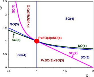
Figure 3: Phase diagram of TQD.

The central domain of dimension $T_{K0}$ describes the fully symmetric state (8), and various regimes of Kondo tunneling correspond to lines or segments in the $\{x,y\}$ plane. Vertically hatched domain corresponds to TQD with singlet ground state where the Kondo effect is absent. Experimental test is suggested in Fig. 4 which illustrates the evolution of $T_{K}$, with $\delta_{rl}\sim y$ for $x=0.96$ and $x=0.7$ corresponding to a symmetry change from $\hat{P}\times SO(4)\times SO(4)$ to $\hat{P}\times SO(3)\times SO(3)$ and from $SO(5)$ to $SO(4)$, respectively.

In similarity with planar QDs or DQDs with $SO(4)$ symmetry Misha ; Eto ; KA01 ; KA02 , Kondo tunneling may be induced by external magnetic field $B$ also in the non-magnetic sector of the phase diagram of Fig. 3 close to the $SO(5)$ line. In this sector $\bar{\delta}=E_{S_{l,r}}-E_{T}<0$, and the Kondo effect emerges when the Zeeman splitting energy $E_{z}=g\mu_{B}B\approx\bar{\delta}$. Due to this compensation $E_{T1}\approx E_{S_{l,r}}$ and the spin Hamiltonian confined to this subspace has a form of anisotropic $SU(2)$ Kondo Hamiltonian

$$\widetilde{H}_{int}=J_{\parallel}R_{z}s_{z}+J_{\perp}\left(R^{+}s^{-}+R^{-}s^{+}\right)/2.$$ (15)

Here $J_{\parallel}({\bar{D}})=J^{T}_{l}$, $J_{\perp}({\bar{D}})=\sqrt{2[(\alpha_{l}J^{T}_{l})^{2}+(\alpha_{r}J_{lr})^{2}]}$. The vector $\bf R$ is defined as,

$$R^{+}=\sum_{a}A_{a}X^{1_{l}S_{a}},\;R^{-}=(R^{+})^{\dagger},$$ (16)

$$R_{z}=[X^{1_{l}1_{l}}-\sum_{a}(A_{a}^{2}X^{S_{a}S_{a}}+A_{a}A_{\bar{a}}X^{S_{a}S_{\bar{a}}})]/2,$$

where $A_{l}=\sqrt{2}\alpha_{l}J_{\parallel}({\bar{D}})/J_{\perp}({\bar{D}})$, $A_{r}=\sqrt{2}\alpha_{r}J_{lr}/J_{\perp}({\bar{D}})$, $A_{l}^{2}+A_{r}^{2}=1,$ and $[R_{j},R_{k}]=ie_{jkm}R_{m}.$ The operators (16) generate the algebra $o_{3}$ in the spin subspace $\{S_{l},S_{r},T1_{l}\}$ specified by the Casimir operator $R^{2}=(3/4)[X^{1_{l}1_{l}}+\sum_{a}(A_{a}^{2}X^{S_{a}S_{a}}+A_{a}A_{\bar{a}}X^{S_{a}S_{\bar{a}}})].$ The scaling equations for dimensionless exchange constants read,

$$dj_{\parallel}/d\ln d=-(j_{\perp})^{2},\;\;\;\;dj_{\perp}/d\ln d=-j_{\parallel}j_{\perp},$$ (17)

yielding the Kondo temperature,

$$T_{Kz}=\bar{D}\exp\left[-\frac{1}{C}\left(\frac{\pi}{2}-\arctan\left(\frac{j_{\parallel}}{C}\right)\right)\right],$$ (18)

where $C=\sqrt{(2\alpha_{l}^{2}-1)(j_{\parallel})^{2}+2(\alpha_{r}j_{lr})^{2}}$.

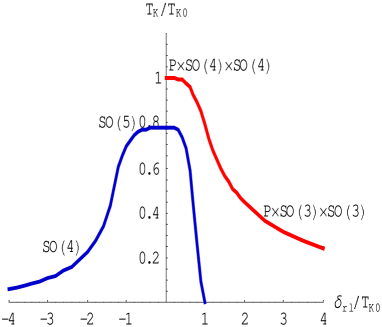
Figure 4: Kondo temperature

Another type of field induced Kondo effect is realized in symmetric case of $\bar{\delta}=E_{S_{l,r}}-E_{T_{l,r}}<0$. Now two components of a triplet, namely $E_{T1_{l,r}}$ cross with two singlet states, and the symmetry group of the TQD is $SO(4)$. The $o_{4}$ algebra is formed by two vectors ${\bf R}$ and $\hat{P}{\bf R}$ which intermix the states $S_{l,r}$ and $T_{l,r}$. The Kondo Hamiltonian is also anisotropic. RG procedure similar to (17) yields the Kondo temperature

$$T_{Kz}=\bar{D}\exp\left[-\frac{1}{2C}\left(\frac{\pi}{2}-\arctan\left(\frac{j^{T}}{C}\right)\right)\right],$$ (19)

where $C=\sqrt{(2\alpha^{2}-1)(j^{T})^{2}}$.

To conclude, the dynamical $SO(n)$ symmetry of Kondo tunneling through an evenly occupied TQD is unraveled. It is found that the Kondo resonance with variable $T_{K}$ arises due to strong correlations in a central well, which plays a role of side-coupled dot for both left and right wells. The hidden dynamical symmetry manifests itself, firstly in the very existence of the Kondo effect in QDs with even ${\cal N}$, secondly in non-universal $T_{K}$. Its dependence on the ratios $x,y$ of the gate voltages and tunneling rate may be observed as peculiar conductance curve $g(x,y)$ at low temperature in specific Coulomb blockade windows, following the curve $T_{K}(x,y)$ exemplified in Figs. 3,4. In a singlet spin state the anisotropic Kondo effect can be induced in TQD by external magnetic field.

The theory is constructed in a single-channel approximation for lead electrons. In a split gate geometry, more than one tunneling channel may arise. One may anticipate that the peculiar even occupation regime of complex QDs then transforms into conventional odd occupation Kondo regime.

This research is partially supported by ISF, BSF and DIP funds.

References

(1) L. Glazman and M. Raikh, JETP Lett. 47, 452 (1988);
T.K. Ng and P.A. Lee, Phys. Rev. Lett. 61, 1768 (1988); Y.
Meir
N. S. Wingreen, Phys. Rev. Lett. 70, 2601 (1993).
(2) D. Goldhaber-Gordon et al., Nature (London)
391, 156 (1998); S.M. Cronenwett et al., Science
281, 540 (1998); J. Schmid et al., Physica B 256-258, 182 (1998).
(3) M. Pustilnik, Y. Avishai and K. Kikoin, Phys. Rev. Lett.
84,1756 (2000); J. Nygård et al, Nature, 408,
342 (2000); M. Pustilnik and L.I. Glazman, Phys. Rev. B 64,
045328 (2001), M. Eto and Yu. V. Nazarov, Phys. Rev. B64,
085322 (2001).
(4) N.S. Sasaki et al, Nature, 405, 764 (2000);
M. Eto and Yu. V. Nazarov, Phys. Rev. Lett. 85, 1306 (2000);
M. Pustilnik and L. Glazman, Phys. Rev. Lett. 85, 2993
(2000); D. Guiliano et al, Phys. Rev. B63, 125318 (2001).
(5) K. Kikoin and Y. Avishai, Phys. Rev. Lett.
86, 2090 (2001).
(6) K. Kikoin and Y. Avishai, Phys.
Rev. B 65, 115329 (2002).
(7) A.C. Hewson, The Kondo Effect to Heavy Fermions
(Cambridge University Press, Cambridge, 1993).
(8) F.D.M. Haldane, Phys. Rev. Lett.
40, 416 (1978).