Effective spinless fermions in the strong coupling Kondo model

Abstract

Starting from the two-orbital Kondo-lattice model with classical $t_{2g}$ spins, an effective spinless fermion model is derived for strong Hund coupling $J_{H}$ with a projection technique. The model is studied by Monte Carlo simulations and analytically using a uniform hopping approximation. The results for the spinless fermion model are in remarkable agreement with those of the original Kondo-lattice model, independent of the carrier concentration, and even for moderate Hund coupling $J_{H}$. Phase separation, the phase diagram in uniform hopping approximation, as well as spectral properties including the formation of a pseudo-gap are discussed for both the Kondo-lattice and the effective spinless fermion model in one and three dimensions.

I Introduction

The study of manganese oxides such as La_1-xSr_xMnO₃ (LSMO) and La_1-xCa_xMnO₃ (LCMO) has attracted considerable attention since the discovery of colossal magnetoresistance in these compounds Dagotto et al. (2001); Oleś et al. (2000). These materials crystallize in the perovskite-type lattice structure where the crystal field partially lifts the degeneracy of the manganese d-states. The energetically favorable three-fold degenerate $t_{2g}$ levels are populated with localized electrons, which according to Hund’s rule form localized $S=3/2$ spins. The electronic configuration of the Mn³⁺ ions is $t_{2g}^{3}e_{g}^{1}$ with one electron in the $e_{g}$ orbital, which is missing in the Mn⁴⁺ ions. The $e_{g}$ electrons can move between neighboring Mn ions mediated by bridging $O^{2-}$ $2p$ orbitals. The interplay of electronic, spin, and orbital degrees of freedom along with the mutual interactions, such as the strong Hund coupling $J_{H}$ of the itinerant electron to localized $t_{2g}$ spins, Coulomb correlations, and electron-phonon coupling leads to a rich phase diagram including antiferromagnetic insulating, ferromagnetic metallic, and charge ordered domains Kaplan and Mahanti (1998). Charge carriers moving in the spin and orbital background show interesting dynamical features Horsch et al. (1999); Bala et al. (2002). The electronic degrees of freedom are generally treated by a Kondo-lattice model, which in the strong Hund coupling limit is commonly referred to as double-exchange (DE) model, a term first coined by ZenerZener (1951).

Monte Carlo (MC) simulations have contributed significantly to our understanding of the manganites. Intense MC simulations for the DE model have been performed by Dagotto et al Dagotto et al. (1998) and Furukawa Furukawa (1998) in the space of the classically treated $t_{2g}$ spins. Static and dynamical observables of the Kondo model have been determined Yunoki and Moreo (1998). These MC simulations gave first theoretical indications of phase separation (PS) Yunoki et al. (1998a) in manganite models. Preliminary studies have been performed to analyze the importance of nearest neighbor Coulomb repulsion in the two-orbital DE model Hotta et al. (2000) as well as the importance of classical phonons Yunoki et al. (1998b).

Many publications are based on the $J_{H}=\infty$ limit. Here we propose an effective spinless fermion model for the strong coupling limit of the Kondo-lattice Hamiltonian, which is equally simple as the $J_{H}=\infty$ limit but which still contains the crucial physical ingredients of finite $J_{H}$. The dynamic variables are $e_{g}$ electrons with spins parallel to the $t_{2g}$ spins at the respective sites. The influence of antiparallel spins is accounted for by the effective Hamiltonian. The derivation of the model is based on a projection technique, analogous to the derivation of the $tJ$ model from the Hubbard model. The role of the Hubbard $U$ is played by $J_{H}$ which couples to the classical $t_{2g}$ spins. In contrast to the $tJ$ model, the high-energy subspace is thus controlled by classical variables and consequently the resulting model is much simpler than the $tJ$ model. For a given $t_{2g}$ spin configuration, the resulting Hamiltonian is a one-particle operator. Its electronic trace can be evaluated analytically, once the one-particle energies are known, leading to an effective action for the $t_{2g}$ spins, which can be simulated by Monte Carlo techniques.

The obvious advantage of this approach is the reduction of the dimension of the Hilbert space. This can be exploited in MC simulations by going to larger systems and/or additional degrees of freedom.

For a large range of parameters, the effective spinless fermion model is found to yield very satisfactory results and to perform much better than the rough $J_{H}\to\infty$ approximation. We compare spin- and charge-correlations as well as quasi-particle spectra of the projection approach with the full two-spin model and with the $J_{H}\to\infty$ limit.

The effective model is treated without approximations by Monte Carlo simulations as well as by a uniform hopping approximation (UHA) capturing the essential influence of the $t_{2g}$ spins on the $e_{g}$ electrons. The UHA computation can be performed analytically, particularly in the thermodynamic limit. Most of the UHA results are found to be in striking agreement with MC results. We find two phase transitions as a function of the chemical potential, one close to the empty band and the second close to a completely filled band. At each phase transition we observe PS, as reported for the upper transition in Yunoki et al. (1998a). For a 1D-chain we derive an analytical expression for the two critical chemical potentials at which (PS) occurs.

For the 3D Kondo-lattice model canonical UHA results yield a phase diagram which displays various types of antiferromagnetic (AF) order including spin-canting, as well as ferromagnetism (FM). Our finite $J_{H}$ results for 3D are in close agreement with those derived in the limit of infinite Hund coupling van den Brink and Khomskii (1999). In the grand canonical ensemble we find, however, that only the 3D antiferromagnetic and the 3D ferromagnetic order prevail. The transition is again accompanied by PS.

The paper is organized as follows. In Sec. II the Kondo-lattice model is introduced. By applying a projection technique in Sec. III this model is mapped onto the effective spinless fermion model. In Sec. IV we present the phase diagrams and phase separation boundaries in one and three dimensions within a uniform hopping approximation. Results of Monte Carlo simulations for the original and the projected model are discussed in Sec. V. Finally, in Sec. VI we summarize the key conclusions.

II Model Hamiltonian

In this paper, we will concentrate on purely electronic ($t_{2g},e_{g}$) properties, leaving phonon degrees of freedom for further studies. As proposed by Dagotto et al. Dagotto et al. (1998) and Furukawa Furukawa (1998), the $t_{2g}$ spins $\mathbf{S}_{i}$ are treated classically, which is equivalent to the limit $S\to\infty$. The spin degrees of freedom are therefore replaced by unit vectors $\mathbf{S}_{i}$, parameterized by polar and azimuthal angles $\theta_{i}$ and $\phi_{i}$, respectively, that represent the direction of the $t_{2g}$ spin at lattice site $\mathbf{x}_{i}$. The magnitude of the spin is absorbed into the exchange couplings. It is expedient to use the individual $t_{2g}$ spin directions as local quantization axes for the spin of the itinerant $e_{g}$ electrons at the respective sites. This representation is particularly useful for the $J_{H}\to\infty$ limit, but also for the projection technique, which takes spin-flip processes for finite Hund coupling into account.

It is commonly believed that the electronic degrees of freedom are well described by a multi-orbital Kondo-lattice model

$$\hat{H}=-\sum_{i,j,\alpha,\beta,\sigma,\sigma^{\prime}}\;t^{\sigma,\sigma^{\prime}}_{i\alpha,j\beta}\;c^{\dagger}_{i\alpha\sigma}\,c^{\phantom{\dagger}}_{j\beta\sigma^{\prime}}+2J_{H}\sum_{i\alpha}\hat{n}_{i\alpha\downarrow}+J^{\prime}\sum_{<ij>}\mathbf{S}_{i}\cdot\mathbf{S}_{j}\;.$$ (1)

It consists of a kinetic term with modified transfer integrals $t_{i\alpha,j\beta}^{\sigma,\sigma^{\prime}}$, where $i(j)$ are site-, $\alpha(\beta)$ orbital-, and $\sigma(\sigma^{\prime})$ spin indices. The number of lattice sites will be denoted by $L$ and the number of orbitals per site by $M$. The operators $c^{\dagger}_{i\alpha\sigma}(c^{\phantom{\dagger}}_{i\alpha\sigma})$ create (annihilate) $e_{g}$-electrons at site $x_{i}$ in the orbital $\alpha$ with spin parallel ($\sigma=\uparrow$) or anti-parallel ($\sigma=\downarrow$) to the local $t_{2g}$ spin orientation $\mathbf{S}_{i}$. The next term describes the Hund coupling with exchange integral $J_{H}$. As usual, $\hat{n}_{i\alpha\sigma}$ is the spin-resolved occupation number operator. Usually, the Kondo-lattice Hamiltonian contains an additional term proportional to the electron number $\hat{N}_{e}$, $\hat{H}_{c}=-J_{H}\hat{N}_{e}$, which has been omitted in Eq. (1), as it merely results in a trivial shift of the chemical potential $\mu\to\mu-J_{H}$.

The modified hopping integrals $t^{\sigma,\sigma^{\prime}}_{i\alpha,j\beta}$ depend upon the geometry of the $e_{g}$-orbitals and the relative orientation of the $t_{2g}$ spins:

$$t^{\sigma,\sigma^{\prime}}_{i\alpha,j\beta}\;=\;t_{i\alpha,j\beta}\;u_{ij}^{\sigma,\sigma^{\prime}}\;.$$

The first factor on the RHS is given by the hopping amplitudes $t_{i\alpha,j\beta}$ which read

$$t_{i,i+\hat{z}}\;=\;t\;\left(\begin{array}[]{cc}0&0\\ 0&1\end{array}\right),\;t_{i,i+\hat{x}/\hat{y}}=t\;\left(\begin{array}[]{cc}\tfrac{3}{4}&\mp\tfrac{\sqrt{3}}{4}\\ \mp\tfrac{\sqrt{3}}{4}&\tfrac{1}{4}\end{array}\right)$$ (2)

as matrices in the orbital indices $\alpha,\beta=1(2)$, corresponding to the $x^{2}-y^{2}$ ($3z^{2}-r^{2}$) orbitals (see e.g. Dagotto et al. (2001)). The overall hopping strength is $t$, which will be used as unit of energy, by setting $t=1$. The relative orientation of the $t_{2g}$ spins at site $i$ and $j$ enters via

$$\begin{aligned} u^{\sigma,\sigma}_{i,j}&=c_{i}c_{j}+s_{i}s_{j}\;e^{i\sigma(\phi_{j}-\phi_{i})}\\ u^{\sigma,-\sigma}_{i,j}&=\sigma(c_{i}s_{j}\;e^{-i\sigma\phi_{j}}-c_{j}s_{i}\;e^{-i\sigma\phi_{i}})\end{aligned}\;,$$ (3)

with the abbreviations $c_{j}=\cos(\theta_{j}/2)$ and $s_{j}=\sin(\theta_{j}/2)$ and the restriction $0\leq\theta_{j}\leq\pi$. The modified hopping part of the Hamiltonian is still hermitian, since $u_{i,j}^{\sigma,\sigma^{\prime}}=\big{(}u_{j,i}^{\sigma^{\prime},\sigma}\big{)}^{*}$.

Finally, Eq. (1) contains a super-exchange term. The value of the exchange coupling is $J^{\prime}\approx 0.02$ Dagotto et al. (2001), accounting for the weak antiferromagnetic coupling of the $t_{2g}$ electrons. Here we will approximate the local $t_{2g}$ spins classically. For strong Hund coupling $J_{H}\gg 1$ the electronic density of states (dos) consists essentially of two sub-bands, a lower and an upper ’Kondo-band’, split by approximately $2J_{H}$. In the lower band the itinerant $e_{g}$ electrons move such that their spins are predominantly parallel to the $t_{2g}$ spins, while the opposite is true for the upper bandvon der Linden and Nolting (1982). Throughout this paper, the electronic density $n$ (number of electrons per site) will be restricted to $0\leq n\leq 1$, i.e. predominantly the lower Kondo-band is involved.

III Projection Technique

The separation of energy scales Auerbach (1994) is a well known strategy to simplify quantum-mechanical many-body systems. In the case of manganites, the Hund coupling $J_{H}$ is known to be much greater than the other parameters $t$ and $J^{\prime}$. Consequently, the hopping to antiparallel $e_{g}-t_{2g}$ configurations can be treated in second order perturbation theory Shen and Wang (2000); Yarlagadda and Ting (2001) by a projection approach. On the low energy scale, the dynamical variables are $e_{g}$ electrons with spin parallel to the local $t_{2g}$ spins. The virtual excitations $(i\alpha\uparrow)\to(j\beta\downarrow)\to(i^{\prime}\alpha^{\prime}\uparrow)$, which are mediated by the hopping matrix, lead to an effective spinless fermion Hamiltonian

$$\hat{H}_{p}=-\sum_{i,j,\alpha,\beta}t^{\uparrow\uparrow}_{i\alpha,j\beta}\,c^{\dagger}_{i\alpha}\,c^{\phantom{\dagger}}_{j\beta}-\sum_{i,\alpha,\alpha^{\prime}}\bigg{(}\sum_{j,\beta}\frac{t^{\uparrow\downarrow}_{i\alpha^{\prime},j\beta}\,t^{\downarrow\uparrow}_{j\beta,i\alpha}}{2J_{H}}\bigg{)}c^{\dagger}_{i\alpha^{\prime}}c^{\phantom{\dagger}}_{i\alpha}-\sum_{[i\neq i^{\prime}],\alpha,\alpha^{\prime}}\!\!\!\bigg{(}\sum_{j,\beta}\frac{t^{\uparrow\downarrow}_{i^{\prime}\alpha^{\prime},j\beta}\,t^{\downarrow\uparrow}_{j\beta,i\alpha}}{2J_{H}}\bigg{)}c^{\dagger}_{i^{\prime}\alpha^{\prime}}c^{\phantom{\dagger}}_{i\alpha}+J^{\prime}\sum_{<ij>}\mathbf{S}_{i}\cdot\mathbf{S}_{j}\;.$$ (4)

The effective Hamiltonian contains the kinetic energy of $e_{g}$ electrons with spin parallel to the $t_{2g}$ spins (first term). The kinetic energy is optimized by aligning all $t_{2g}$ spins which is the usual ferromagnetic double exchange effect. The second term describes an additional hybridization and favors antiferromagnetic $t_{2g}$ spins leading to an effective antiferromagnetic interaction $J_{\text{eff}}$ which is generally stronger than $J^{\prime}$. The “three-site” hopping processes of the third term are of minor influence. We will see that this term is in general negligible. On the other hand, its inclusion does not really increase the numerical effort. Eq. (4) is valid for arbitrary hopping matrices $t_{i\alpha,j\beta}$. In subsequent sections, however, the discussion will be restricted to nearest-neighbor hopping only.

The Hamiltonian Eq. (4) constitutes a spinless fermion model, similar to the one obtained in the $J_{H}\to\infty$-limit, which can be treated numerically along the lines proposed by Dagotto and coworkers Dagotto et al. (1998) and Furukawa Furukawa (1998). Finite $J_{H}$ values can thus be treated with the same numerical effort as the case $J_{H}=\infty$. In the MC simulations the weight for a $t_{2g}$ spin configuration is determined by the grand canonical trace over the fermionic degrees of freedom in the one-electron potential created by the $t_{2g}$ spins.

The obvious advantage of Eq. (4) as compared to Eq. (1) is the reduced Hilbert space.

IV Uniform Hopping approximation

Before discussing approximation-free MC results for the effective spinless fermion model, we will investigate the main features of the Hamiltonian (4) by a uniform hopping approximation proposed by van-den-Brink and Khomskiivan den Brink and Khomskii (1999). To this end, we introduce two different mean angles between neighboring $t_{2g}$ spins, one in $z$-direction ($\theta_{z}$) and one in the $xy$-plane ($\theta_{xy}$). It should be stressed that $\theta_{z}$ and $\theta_{xy}$ are relative angles between adjacent spins, with values between $0$ and $\pi$, and are not to be confused with the polar angles $\theta_{i}$. We assume that these angles are the same between all neighbor spins, i.e. $\mathbf{S}_{i}\cdot\mathbf{S}_{i\pm\hat{z}}=\cos\theta_{z}$ for all lattice sites $i$ and $\mathbf{S}_{i}\cdot\mathbf{S}_{i\pm\hat{x}}=\mathbf{S}_{i}\cdot\mathbf{S}_{i\pm\hat{y}}=\cos\theta_{xy}$. The allowed spin configurations include, among others, ferro- and antiferromagnetism as well as spin canted states. The impact of the $t_{2g}$ spins on the hopping amplitudes simplifies to

$$u^{\sigma,\sigma}_{z}=\cos(\frac{\theta_{z}}{2})\quad,\qquad u^{\sigma,-\sigma}_{z}=\sin(\frac{\theta_{z}}{2})\;.$$

for hopping processes along the $z$-direction and similarly for $u^{\sigma,\sigma^{\prime}}_{xy}$ for electron motion in the $xy$-plane. The hopping matrix is now translationally invariant. The inner product of the $t_{2g}$ spins entering the super-exchange reads

$$\mathbf{S}_{i}\cdot\mathbf{S}_{i+\hat{z}}=\cos\theta_{z}=2u_{z}^{2}-1$$

and similarly for neighboring pairs in the $xy$-plane.

IV.1 Phase Separation in 1D systems

First we consider the simplest case, namely a 1D chain in $z$-direction and we ignore the additional three-site hopping (third term in Eq. (4)). At the end of this section we will show that it can indeed be neglected. Due to the symmetry of the hopping elements the $x^{2}-y^{2}$-orbitals form an irrelevant dispersionless band, which will be ignored in the sequel. The influence of the average spin orientation is captured in the uniform hopping amplitude $u$. Assuming periodic boundary conditions, the Hamiltonian simplifies to

$$\hat{H}=-u\sum_{\langle ij\rangle}c^{\dagger}_{i}c^{\phantom{\dagger}}_{j}-\frac{1-u^{2}}{J_{H}}\,\sum_{i}c^{\dagger}_{i}c^{\phantom{\dagger}}_{i}+J^{\prime}L\big{(}2u^{2}-1\big{)}\;,$$ (5)

where we have dropped orbital indices. The virtual hopping processes couple merely to the density and the dispersion of the spinless fermions is given by the shifted tight-binding band structure

$$\epsilon_{k}=-2u\cos(k)-(1-u^{2})/J_{H}\;.$$ (6)

The band width is $4u$. It vanishes accordingly for AF order and reaches a maximum for FM order. In Fig. 1 the resulting band-filling is schematically depicted for zero temperature as function of chemical potential and hopping amplitude.

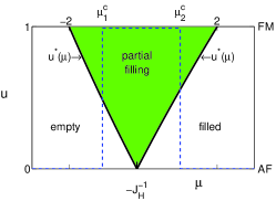
Figure 1: Filling of the tight-binding band depending upon chemical potential and hopping amplitude. Condition for partial filling: $u>u^{*}(\mu)$. The minimum free energy solution in UHA (dashed line) exhibits a jump (phase separation) from AF to FM order at $\mu^{c}_{1}$ and back to AF order at $\mu^{c}_{2}$.

The condition for an empty/ filled band depends on the ’effective chemical potential’

$$\tilde{\mu}:=\big{(}\mu+\tfrac{1}{J_{H}}(1-u^{2})\big{)}/u\;.$$ (7)

According to $\mu<\min_{k}(\epsilon_{k})$, the band is empty if $\tilde{\mu}<-2$. For the completely filled band the condition reads $\tilde{\mu}>2$. Partial filling is possible for intermediate values of the chemical potential ($-2<\mu<2$) if the hopping amplitude exceeds a threshold $u^{*}(\mu)$. The logarithm of the grand canonical partition function reads

$$\ln Y=\sum_{k}\ln\big{(}1+e^{-\beta(\epsilon_{k}-\mu)}\big{)}-\beta J^{\prime}L\big{(}2u^{2}-1\big{)}\;.$$

In the thermodynamic limit ($L\to\infty$) and for $T=0$ the free energy per lattice site is

$$f=uE(\tilde{\mu})-u\;\tilde{\mu}\;N(\tilde{\mu})+J^{\prime}(2u^{2}-1)\;,$$ (8)

with $E(x)$ being the mean kinetic energy and $N(x)$ the mean particle number of a tight-binding band with dispersion $-2\cos(k)$. For $|x|\leq 2$ these quantities are

$$E(x)=-\frac{\sqrt{4-x^{2}}}{\pi}\;,\quad N(x)=\frac{1}{2}+\frac{\arcsin(x/2)}{\pi}\;.$$

The kinetic energy $E(x)$ is zero for the empty band $(x<-2)$, as well as for the completely filled band ($x>2$). The mean particle number $N(x)$ is zero if the band is empty and unity if it is full. Fig. 2 shows the free energy as a function of chemical potential and hopping amplitude $u$. We find local minima at $u=0$ (AF order) and $u=1$ (FM order). The kinetic terms decrease with increasing $u$, favoring FM order, while the $t_{2g}$ spin energies increase with increasing $u$, favoring AF order. The global minimum switches from AF to FM at the critical chemical potential $\mu=\mu^{c}_{1}$ and back to AF at $\mu=\mu^{c}_{2}$.

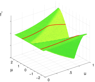
Figure 2: Free energy as a function of chemical potential and hopping amplitude $u$ for $T=0$, $J_{H}=6$ and $J^{\prime}=0.02$. The solid lines are for $\mu^{c}_{1}$ and $\mu^{c}_{2}$, respectively. For the sake of clarity, $f(u=0,\mu)$ has been subtracted.

The values for the critical chemical potential follow from the condition $f|_{u=0}=f|_{u=1}$, yielding

$$(\mu^{c}+1/J_{H})\,N_{0}(\mu^{c})+2J^{\prime}=\mu^{c}\,N(\mu^{c})-E(\mu^{c})\;,$$ (9)

where $N_{0}(\mu^{c})$ denotes the mean particle number for $u=0$, i.e. for perfect AF order. In this case, the tight-binding band is dispersionless and $N_{0}(\mu^{c})$ is either zero or one, depending upon the actual value of the chemical potential.

For the standard parameter set $J_{H}=6$ and $J^{\prime}=0.02$ the numerical values for $\mu^{c}$ are $\mu^{c}_{1}=-1.6730$ and $\mu^{c}_{2}=1.03431$.

The UHA solution corresponds to the global minimum of the free energy. Its location is depicted in Fig. 1 and the corresponding densities are shown as lines in Fig. 3.

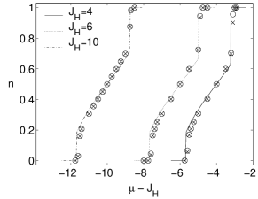
Figure 3: Electron density versus chemical potential for $J_{H}=4,6$, and $10$ (right to left), and $J^{\prime}=0.02$. The lines correspond to UHA. MC results at $\beta=50$, $L=20$ for the spinless fermion model $H_{p}$ (circles) are compared with those for the DE model $H$ (crosses). Error bars of the MC data are smaller than the symbols.

For large negative chemical potential the system is antiferromagnetic and the $e_{g}$ band is empty. At $\mu^{c}_{1}$, AFM domains with zero electron density coexist with FM domains with finite density $n_{1}$. Increasing $\mu$ leads to ferromagnetism, and the filling increases gradually with $\mu$, following the tight binding formula $n=\arccos(-\mu/2)/\pi$.

At $\mu^{c}_{2}$, FM domains with density $n_{2}>n_{1}$ coexist with AFM domains of density one. Finally, for $\mu>\mu^{c}_{2}$, the system jumps back to antiferromagnetism, now at density one. We thus see that the system exhibits phase separation. It should be pointed out that PS is suppressed if nearest-neighbor Coulomb repulsion among $e_{g}$ electrons is included into the model Koller et al. (2002).

Let us now discuss the values of $\mu^{c}_{1,2}$ and the size of the discontinuity in $n$. According to Eq. (9), the first critical chemical potential $\mu^{c}_{1}=\mu^{c}(J^{\prime})$, corresponding to $N_{0}(\mu)=0$, is independent of the actual value of $J_{H}$. Here the effective antiferromagnetic interaction $J_{\text{eff}}$ purely stems from the superexchange coupling of the $t_{2g}$ spins, $J_{\text{eff}}=J^{\prime}$. This does, however, not mean that the Hund coupling is irrelevant for this phase transition. On the contrary, the phase transition is driven by the FM tendency introduced by the Hund coupling. The independence of $J_{H}$ in our results means that there are no second order corrections to the $J_{H}=\infty$ limit. The dependence of $\mu^{c}$ on $J^{\prime}$ is depicted in Fig. 4.

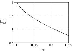
Figure 4: Dependence of the critical chemical potential $|\mu^{c}_{1,2}|$ on the effective exchange coupling $J_{\text{eff}}$.

Now we turn to the second phase transition corresponding to $N_{0}(\mu^{c})=1$. This transition is controlled by the stronger effective exchange coupling

$$J_{\text{eff}}=J^{\prime}+\tfrac{1}{2J_{H}}\;,$$ (10)

as can be seen from Eq. (9), or directly from Eq. (5) at $N=1$. Due to the particle-hole relation $N(-\mu)+N(\mu)=1$ the second critical chemical potential is given by $\mu^{c}_{2}=-\mu^{c}(J_{\text{eff}})$, depicted in Fig. 4. In the limit $J_{H}\to\infty$ we have $\mu^{c}_{1}=-\mu^{c}_{2}$. The density discontinuity is $\Delta n:=N(\mu^{c}_{1})=\Delta n(J^{\prime})$ at $\mu^{c}_{1}$ and $\Delta n:=1-N(\mu^{c}_{2})=\Delta n(J_{\text{eff}})$ at $\mu^{c}_{2}$.

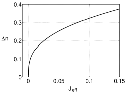
Figure 5: Discontinuity in $n$ as a function of the effective exchange coupling $J_{\text{eff}}$.

It is depicted in Fig. 5. Series expansion of Eq. (9) with respect to $\mu^{c}$ about $\mu^{c}=-2$ yields $\Delta n=(3J^{\prime}/\pi^{2})^{1/3}$. At $J_{\text{eff}}=0$ the slope of the curve diverges, implying that already an infinitesimal $J_{\text{eff}}$ leads to phase separation in this regime.

For realistic parameter values ($J_{H}=6$ and $J^{\prime}=0.02$) we find $\Delta n_{1}\approx 0.18$ and $\Delta n_{2}\approx 0.3$, respectively. The second value is mainly driven by the virtual hopping, which increases the tendency towards PS.

IV.2 Impact of “three-site-terms”

Here we consider the impact of the additional hopping in Eq. (4), which in the 1D case with one orbital results in a next-nearest neighbor hopping

$$\hat{H}^{*}=-\frac{1-u^{2}}{2J_{H}}\,\sum_{i}c^{\dagger}_{i+2}\,c^{\phantom{\dagger}}_{i}+h.c.\qquad.$$

Combined with the terms of Eq. (5), the resulting single-particle dispersion reads

$$\epsilon_{k}=-2u\cos k\;-\;\frac{1-u^{2}}{J_{H}}\;-\;\frac{1-u^{2}}{J_{H}}\,\cos(2k)\;.$$

In the limit $u\to 1$ we recover the original tight-binding band. The density of states has additional van Hove singularities. Contrary to the dispersion of Eq. (5), the band width remains finite in the limit $u\to 0$, due to $\hat{H}^{*}$.

Next we derive the conditions for phase separation. In the limit $T\to 0$, the free energy is given by

$$f=\int_{-\infty}^{\mu}d\epsilon\;\rho_{u}(\epsilon)(\epsilon-\mu)\;-\;J^{\prime}(2u^{2}-1)\;,$$

where $\rho_{u}(\epsilon)$ denotes the density of states corresponding to $\epsilon_{k}$. Numerical evaluation shows that the minima of $f$ are still at $u=0$ and $u=1$. The condition for phase separation is therefore still $f|_{u=0}=f|_{u=1}$. In principle, due to the finite width of the band at $u=0$ intermediate particle numbers $N_{0}(\mu^{c})$ are possible. A detailed calculation shows, however, that for realistic parameters, only $N_{0}(\mu^{c})=0$ or $N_{0}(\mu^{c})=1$ can meet the phase separation criterion. For $N_{0}(\mu^{c})=0$ and $N_{0}(\mu^{c})=1$, however, no hopping is possible and consequently the additional hopping term vanishes. Therefore, the criterion for PS is the same as in Eq. (9) and the three-site hopping has no influence on the critical chemical potentials $\mu_{c}$ at which phase separation occurs.

In general, the modification of the bandwidth due to next-nearest neighbor hopping is small. It has almost negligible impact on the results. On the other hand it poses little extra-effort to include it in MC simulation.

IV.3 Phase Diagram in 3D systems

We now turn to the 3D case. In uniform hopping approximation, the super-exchange reads

$$\hat{H}_{se} =J^{\prime}L^{3}\big{(}2(2u_{xy}^{2}-1)+(2u_{z}^{2}-1)\big{)}\;$$

where $L$ denotes the linear dimensions of the system. Upon substituting uniform hopping amplitudes into Eq. (4), the fermionic part of the Hamiltonian can easily be diagonalized. The one-particle energies are given by the eigenvalues of a $2\times 2$ matrix with matrix elements

$$\epsilon_{11}(k)= \frac{3}{2}\Big{(}-u_{xy}(\cos k_{x}+\cos k_{y})-(1-u_{xy}^{2}))/J_{H}\Big{)}$$ (11)

$$\epsilon_{12}(k)= \frac{\sqrt{3}}{2}\,u_{xy}\big{(}\cos k_{x}-\cos k_{y}\big{)}=\epsilon_{21}(k)$$

$$\epsilon_{22}(k)= -2u_{z}\cos k_{z}-u_{xy}\big{(}\cos k_{x}+\cos k_{y}\big{)}/2$$

$$-\big{(}1-u_{z}^{2}+(1-u_{xy}^{2})/2\big{)}/J_{H}$$

where the subscript $1$ ($2$) refers to $x^{2}-y^{2}$ ($3z^{2}-r^{2}$) orbitals. The symmetry of the $e_{g}$-wavefunction has been exploited in the above expressions. As a consequence of the UHA with two different angles $\theta_{z}$ and $\theta_{xy}$, virtual hopping processes cannot induce transitions between different orbitals, and $J_{H}$ appears only in the diagonal elements of the matrix.

We determine the phase diagram in the canonical ensemble at $T=0$ with respect to electron density $n$ and exchange coupling $J^{\prime}$ for fixed Hund coupling $J_{H}=8$, with Eq. (11) evaluated on a $20^{3}$ momentum lattice. For each parameter set, the free energy is minimized with respect to the hopping amplitudes. The resulting phase diagram is depicted in Fig. 6. At very low doping, 3D antiferromagnetic (G) order dominates, irrespective of the value of $J^{\prime}$, as long as $J^{\prime}>0$. Increasing the electron concentration for $J^{\prime}>0.02$, the system favors first a C-phase, then an A-phase, and finally ferromagnetism (F). Similar results have been found for the $J_{H}=\infty$ limit van den Brink and Khomskii (1999). Finite values for $J_{H}$ have almost negligible influence on the phase diagram for densities $n<0.5$. The G-phase has not been reported in van den Brink and Khomskii (1999) since it has not been taken into consideration.

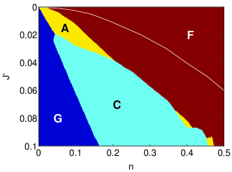
Figure 6: Canonical $T=0$ UHA phase diagram of the spinless two-orbital Kondo-lattice model with classical $t_{2g}$ spins for $J_{H}=8$. Depending upon the electron concentration of the canonical ensemble and the super-exchange, G-type, A-type, C-type antiferromagnetic phases or the ferromagnetic phase (F) are observed. Meaning of phases: G=(AF,AF); A=(FM,AF); C=(AF,FM); F=(FM,FM), where the first entry denotes the order in the xy-plane and the second in z-direction. The solid line represents the phase-boundary between G- and F-order, respectively, obtained in a grand canonical ensemble.

For small super-exchange of the $t_{2g}$ spins ($J^{\prime}<0.018$) the transition from G to A phase evolves via spin canting. By increasing the electron doping, the F-phase is reached without canting. The situation is more complex for larger values of $J^{\prime}$. Fig. 7 shows the optimal angles $\theta_{z}$ and $\theta_{xy}$ as a function of the electron density $n$ for $J^{\prime}=0.025$ and $J_{H}=8$. For $n<0.039$, there is 3D AF order (G-type) with an increasing tendency towards canting between $t_{2g}$ spins in the $xy$ plane. At $n\simeq 0.04$ this tendency is strongly reduced while at the same time $\cos(\theta_{z})$ discontinuously jumps to zero and we gradually enter the C-phase by aligning the spins along the chains in $z$-direction. The ferromagnetic chains are not perfectly antiferromagnetically stacked. At about $8\%$ electron density we observe a phase transition to the A-phase. At $n\approx 0.15$ an abrupt transition to 3D ferromagnetic order occurs.

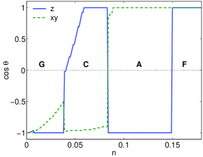
Figure 7: Evolution of the optimal angles $\theta_{z}$ and $\theta_{xy}$ as function of the electron density $n$ at $J^{\prime}=0.025$, $J_{H}=8$. Further details like in Fig. 6.

Besides the analysis for the canonical ensemble, computations have been performed for the grand canonical ensemble as well. The results are significantly different. In the grand canonical ensemble only the $G$ and the $F$ phase remain. The white solid line in Fig. 6 represents the phase boundary between the two phases. For fixed $J^{\prime}$, the behavior is similar to that of the 1D system, depicted in Fig. 3. Below a critical chemical potential $\mu^{c}_{1}$ the electron density is zero and the $t_{2g}$ spins have AF order. At $\mu=\mu^{c}_{1}$, zero density and a finite density $n_{1}$, given by the solid line in Fig. 6, coexist. Concurrently with phase separation, AF- and FM order coexist. Above $\mu^{c}_{1}$ the density increases monotonically. The second transition at $\mu^{c}_{2}$ is not shown in Fig. 6 as it occurs close to $n=1$. Therefore, the grand canonical UHA result does not exhibit the additional magnetic phases (A and C), which are observed in experiment. The relevant densities are never stabilized.

V MC simulations for 1D systems

In this section we compare MC results, obtained for the original double exchange (DE) model (1), with those for the effective spinless fermion model (Eq. (4)), where the additional (“three-site”) hopping term has been neglected. We use the grand canonical Monte Carlo method introduced in Yunoki et al. (1998a) with open boundary conditions (obc).

We restrict the discussion to 1D systems. There is no reason to believe that the performance of the approximation of effective spinless fermions is different in higher dimensions. Furthermore, the approximation has little influence on the orbital degrees of freedom and we restrict the analysis to the one-orbital model. In all simulations, the super-exchange coupling of the $t_{2g}$ spins is $J^{\prime}=0.02$.

Fig. 3 shows the dependence of the electron density on the chemical potential. The system parameters are $L=20$, $\beta=50$, and $J_{H}$ is varied between $J_{H}=4$ and $J_{H}=10$. All results for the two models are in almost perfect agreement. The ’largest’ difference can be observed at $\mu^{c}_{2}$ for $J_{H}=4$. The lines in Fig. 3 represent the results of the uniform hopping approximation, which are strikingly close to the MC data points. The discontinuities are more pronounced in UHA than in the MC data, which can partially be attributed to the fact that the UHA results are for $L=\infty$ and $T=0$. The treatment of finite temperatures in the UHA requires the determination of the number of $t_{2g}$ configurations at a given $u$ and is the subject of current investigations Koller et al. (2002).

The structure factor of the $t_{2g}$ spins has been calculated for various densities $n$ in the grand canonical ensemble by adjusting the chemical potential. The results are illustrated in Fig. 8. Again the data for the two models, Kondo- and effective spinless fermion model, are in perfect agreement within the error bars. Corroborating the UHA results of the previous section, the filled band ($n=1$) has a peak at $k=\pi$, corresponding to AF order. For decreasing density the ferromagnetic peak increases up to $n=1/2$ and then it decreases again. The inset shows the nearest neighbor and next nearest neighbor spin correlation function versus density. We observe that both models yield the same magnetic behavior: AF order at low and high density and a ferromagnetic phase at intermediate fillings. The pronounced peak at $k=\pi$ for $n=1$ results from (virtual) spin-flip processes, driven by the relatively strong exchange coupling $J_{\text{eff}}=0.103$, Eq. (10). Contrariwise, the AF structure near $n=0$ is much less pronounced as it is merely driven by the weak super-exchange coupling $J^{\prime}=0.02$.

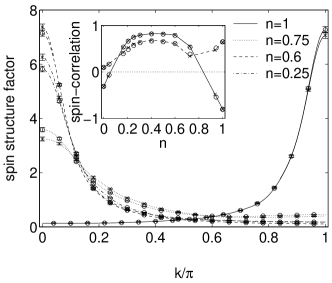
Figure 8: Structure factor for the $t_{2g}$ spins at various electron densities with $J_{H}=6$, $\beta=50$, and $L=20$, for the spinless fermion model $H_{p}$ (circles), and for the DE model $H$ (crosses). When not shown, error bars are smaller than the symbols. The inset shows the nearest neighbor (solid line) and next nearest neighbor (dashed line) $t_{2g}$ spin correlation.

Fig. 9 shows the structure factor for the $t_{2g}$ spins at $n=1$ for different values of $J_{H}$. The AF peak decreases with increasing $J_{H}$ and degenerates to a broad structure in the limit $J_{H}\to\infty$. Obviously, the inclusion of the second order term to the effective spinless fermion model, which is missing in the commonly used $J_{H}=\infty$ limit, and which provides the strong exchange coupling $J_{\text{eff}}$, is crucial for the correct description of the AF order at high electron density. The inset shows the spin structure for $n\approx 3/4$, at which the system exhibits ferromagnetic order. In this case, the FM correlations increase with increasing $J_{H}$.

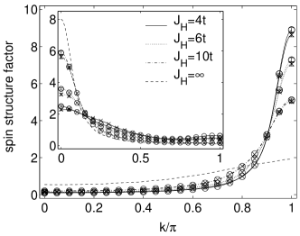
Figure 9: Spin structure factor at $n=1$ (inset: $n\approx 0.75$) for different values of $J_{H}$. Same symbols and parameters as in Fig. 8. In the limit $J_{H}\to\infty$ (dashed line) the intensity of the AF peak is considerably reduced.

Figure 10: Electronic contribution to the total energy versus electron number for $\beta=50$, $L=20$, and $J_{H}=6$. Results for the DE model $\hat{H}$ (crosses) are compared with those for the spinless fermion model $\hat{H}_{p}$ (circles).

As a further test for the spinless fermion model, the electronic contribution to the total energy is shown in Fig. 10. The energy for the Kondo-lattice model (first two terms in Eq. (1)) is compared with the corresponding contributions in the effective spinless fermion model (Eq. (4)). For all fillings the results are in very good agreement.

Quantitatively, the largest differences are found for $n=1$. For this density the dependence of the energy on $J_{H}$ is studied in Fig. 11.

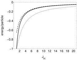
Figure 11: Electronic energies versus Hund coupling $J_{H}$ for a completely filled $20$-site chain at $T=0$. Kinetic energy (dotted line) and total electronic energy (dashed lines) for the Kondo-lattice model. The solid line represents the total electronic energy for the effective spinless fermion model.

A detailed comparison reveals that the effective model describes the electronic energy extremely well, even in the moderate coupling regime. The ubiquitous $J_{H}=\infty$ approximation, on the other hand, yields zero electronic energy. For the parameters underlying Fig. 11, the $t_{2g}$ spins are antiferromagnetically ordered and the lower Kondo-band, or rather the single band of the spinless fermion model, is completely filled. Nevertheless, the kinetic electronic energy is finite due to (virtual) spin-flip processes. It should be pointed out that the additional (three-site) hopping term in Eq. (4) has no influence on this result as the band is entirely filled.

Next we study the spectral function $A_{k}(\omega)$ in the grand canonical ensemble for various mean electron densities covering the regimes for AF and FM order, as well as phase separation. In all cases the system geometry is a 20-site chain with open boundary conditions at inverse temperature $\beta=50$, and exchange couplings $J^{\prime}=0.02$, and $J_{H}=6$. We start out with the spectra in Fig. 12 for strong FM order at a mean particle density of $n=1/2$. According to the inset of Fig. 8 the spin-correlations are 0.82 and 0.67 for nearest and next-nearest neighbors, respectively.

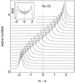
Figure 12: Spectral function obtained by a grand canonical simulation for $n=1/2$ with $J_{H}=6$, $L=20$ and $\beta=50$. An intrinsic linewidth $\gamma=0.1$ has been added. The results for the Kondo model and the effective spinless fermion model are indistinguishable.

The spectral function, depicted in Fig. 12, resembles closely that of a tight-binding model, valid for perfect FM order. The band-width is slightly reduced, and for $k$-values close to the Fermi momentum, $A_{k}(\omega)$ exhibits some minor shoulders. The width (HWHM) of the peaks agrees with $\gamma$, the value by which the finite-size delta peaks have been broadened. The inset displays the density of states (dos), which agrees with the tight-binding density of states for open boundary conditions.

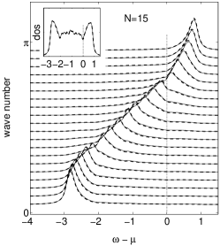
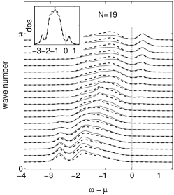
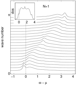
Figure 13: Same as Fig. 12. The indicated particle numbers correspond to $n=0.75$ $n=0.95$, and $n=0.05$. Results for the Kondo model are represented by solid lines and those for the effective spinless fermion model by dashed lines.

Next we increase the mean density to $n=0.75$, corresponding to a chemical potential close to $\mu^{c}_{2}$. The spin order is still predominantly ferromagnetic. The results in Fig. 13 show that both models yield very similar results, namely a tight-binding type of quasi-particle band. The spectral peaks are, however, significantly broader than the mock width $\gamma$ and upon approaching the Fermi momentum the width increases asymmetrically towards the Fermi level. The origin of the broad structures are the random deviations of the $t_{2g}$ spins from perfect FM order. The resulting density of states has piled up spectral weight in the center and reveals a precursor of a pseudo-gap at the Fermi energy. Interestingly, the dos is almost center-symmetric and a mirror image of the ’pseudo-gap’ occurs also at the lower band edge.

The next panel depicts results for $n=0.95$, correspond to a chemical potential slightly above $\mu_{c2}$, where the spin order is predominantly antiferromagnetic. Now the pseudo-gap, as discussed by Moreo et al. Moreo et al. (1999), is clearly visible. Additionally, we observe a ’mirror pseudo-gap’ at the lower band edge. There is still good qualitative agreement between the results of the two models. Quantitatively, however, there are deviations in the structures below the pseudo-gap. The density of states is still remarkably well described by the spinless fermion model.

In the opposite limit of low carrier concentration ($n=0.05$), the chemical potential is close to $\mu_{c1}$, where we find similar features. Again, together with the coexistence of FM and AFM order a pseudo-gap shows up at the chemical potential as well as at the upper band edge. The pseudo-gap is less pronounced in this case, where the antiferromagnetic exchange coupling $J^{\prime}$ is much smaller than $J_{\text{eff}}$ at $\mu^{c}_{2}$.

In both models a considerable amount of spectral weight is transferred from the band edges to the center. Interestingly, the density of states is almost center-symmetric. The pseudo-gap is present in the spectral function irrespective of the wave vector $k$. Moreo et al. argued that the pseudo-gap is formed due to the presence of mixed phases with irregular formations of FM domains. In contrast to this interpretation, we find the pseudo-gap also in the perfect AF regime with a single electron (hole).

Generally we observe, in agreement with ARPES experiments Dessau et al. (1998), that the width of peaks increases towards the Fermi energy and the spectral intensity decreases since spectral weight is transferred to the unoccupied part of the spectrum, which is not visible in ARPES. Furthermore, the peaks are generally much broader than the experimental resolution.

VI Conclusions

We have developed an effective spinless fermion model for the strong coupling multi-orbital Kondo-lattice model. The effective model has a reduced Hilbert space and is particularly suitable for MC simulations. The numerical complexity is the same as that of the $J_{H}=\infty$ model. The reduced Hilbert space allows one to study higher spatial dimensions and/or additional degrees of freedom, such as phonons.

Based on the evaluation of various observables the effective spinless fermion model performs strikingly well, even for moderate Hund coupling.

It appears that virtual spin-flip processes included in our approach, which are missing in the $J_{H}=\infty$ model, are crucial for the antiferromagnetic phase close to half-filling ($n=1$), where they provide a strong effective exchange coupling $J_{\text{eff}}=J^{\prime}+\frac{1}{2J_{H}}$.

Two phase transitions from AF- to FM-order and vice versa are observed, accompanied by phase separation. Analytic expressions for the chemical potential at which phase separation occurs in a 1D chain have been derived in uniform hopping approximation (UHA). It has been shown, however, that they are in extremely good agreement with approximation-free MC results.

The UHA phase diagram of the 3D spinless fermion model has been determined. In canonical ensembles, the magnetic phase diagram is in qualitative agreement with that obtained in previous studies for the $J_{H}=\infty$ limit. Experimentally observed phases, like G-, A-, C-, and F-order are found. On the other hand, grand canonical ensemble calculations show that only 3D AF and 3D FM order prevail. The transition between the two phases is accompanied by phase separation. Densities, required for other phases, are not stable in UHA.

The spectral functions show a remarkable center-symmetry. In the AF phase, at low and high electron density, a pseudo-gap structure is observed at the chemical potential and a mirror image at the opposite edge of the spectrum.

In passing, it should be noted that nearest-neighbor Coulomb repulsion of the $e_{g}$-electrons in a two-orbital model can be detrimental for phase separation. Detailed results will be discussed elsewhere Koller et al. (2002).

VII Acknowledgments

This work was partially supported by the Austrian Science Fund (FWF), project P15834-PHY.

References

- Dagotto et al. (2001) E. Dagotto, T. Hotta, and A. Moreo, Phys. Reports 344, 1 (2001).
- Oleś et al. (2000) A. M. Oleś, M. Cuoco, and N. B. Perkins, in AIP Conference Proceedings (2000), vol. 527, pp. 226–380.
- Kaplan and Mahanti (1998) T. Kaplan and S. Mahanti, Physics of Manganites (Kluwer Academic/ Plenum Publishers, New York, Boston, Dordrecht, London, Moscow, 1998), 1st ed.
- Horsch et al. (1999) P. Horsch, J. Jaklic, and F. Mack, Phys. Rev. B 59, R14149 (1999).
- Bala et al. (2002) J. Bala, A. M. Oles, and P. Horsch, Phys. Rev. B 65, 134420/1 (2002).
- Zener (1951) C. Zener, Phys. Rev. 82, 403 (1951).
- Dagotto et al. (1998) E. Dagotto, S. Yunoki, A. L. Malvezzi, A. Moreo, J. Hu, S. Capponi, D. Poilblanc, and N. Furukawa, Phys. Rev. B 58, 6414 (1998).
- Furukawa (1998) N. Furukawa, in: Physics of manganites (Kluwer Academic Publisher, New York, 1998), 1st ed.
- Yunoki and Moreo (1998) S. Yunoki and A. Moreo, Phys. Rev. B 58, 6403 (1998).
- Yunoki et al. (1998a) S. Yunoki, J. Hu, A. L. Malvezzi, A. Moreo, N. Furukawa, and E. Dagotto, Phys. Rev. Lett. 80, 845 (1998a).
- Hotta et al. (2000) T. Hotta, A. L. Malvezzi, , and E. Dagotto, Phys. Rev. B 62, 9432 (2000).
- Yunoki et al. (1998b) S. Yunoki, A. Moreo, and E. Dagotto, Phys. Rev. Lett. 81, 5612 (1998b).
- van den Brink and Khomskii (1999) J. van den Brink and D. Khomskii, Phys. Rev. Lett 82, 1016 (1999).
- von der Linden and Nolting (1982) W. von der Linden and W. Nolting, Z. Phys. B 48, 191 (1982).
- Auerbach (1994) A. Auerbach, Interacting Electrons and Quantum Magnetism (Springer-Verlag, New York, Berlin, Heidelberg, 1994), 1st ed.
- Yarlagadda and Ting (2001) S. Yarlagadda and C. S. Ting, Int. J. Mod. Phys. B 15, 2719 (2001).
- Shen and Wang (2000) S.-Q. Shen and Z. D. Wang, Phys. Rev. B 61, 9532 (2000).
- Koller et al. (2002) W. Koller, A. Prüll, H. G. Evertz, and W. von der Linden (2002), in preparation.
- Moreo et al. (1999) A. Moreo, S. Yunoki, and E. Dagotto, Phys. Rev. Lett. 83, 2773 (1999).
- Dessau et al. (1998) D. S. Dessau, T. Saitoh, C. H. Park, Z. X. Shen, P. Villella, N. Hamada, Y. Moritomo, and Y. Tokura, Phys. Rev. Lett. 81, 192 (1998).