Many-body approach to spin-dependent transport in quantum dot systems

Abstract

By means of a diagram technique for Hubbard operators we show the existence of a spin-dependent renormalization of the localized levels in an interacting region, e.g. quantum dot, modeled by the Anderson Hamiltonian with two conduction bands. It is shown that the renormalization of the levels with a given spin direction is due to kinematic interactions with the conduction sub-bands of the opposite spin. The consequence of this dressing of the localized levels is a drastically decreased tunneling current for ferromagnetically ordered leads compared to that of paramagnetically ordered leads. Furthermore, the studied system shows a spin-dependent resonant tunneling behaviour for ferromagnetically ordered leads.
PACS numbers: 72.25.-b, 73.23.-b, 73.63.-b

Spin-dependent tunneling [1] and tunneling magneto resistance (TMR) [2, 3] have recently been studied extensively. Concerning spin-dependent tunneling through a quantum dot (QD), or similar interacting regions, the main focus has been to investigate the effects of a magnetic field applied over the interacting region [4, 5, 6, 7]. The opportunity of changing the magnetic properties of the leads, leading in and out of the QD, by an external magnetic field or by spin injection and thereby altering the output current, has so far been a peripheral topic. There are theoretical reports of spin filters and spin memories [8] in which the spin polarized current is controlled by the Zeeman splitting of the localized levels in the QD. Another suggestion is a three-terminal system in which two of the leads are in anti-ferromagnetic order [9]. The source-drain current is manipulated by the magnetization direction in the third terminal. However, these studies are formulated in terms of single-electron properties and, in addition, they cannot be directly transformed into a time-dependent situation. To our knowledge, there is no theoretical report of inducing a large spin-polarization in the QD by simply spin-polarizing the conduction band.

In this Letter we demonstrate, from a many-body approach, that there is a large spin-dependent renormalization of the levels in an interacting region, e.g. a QD, due to the magnetic properties of the leads, which could be used in magnetic sensor applications. By shifting the magnetic ordering in the leads, from paramagnetic to ferromagnetic, the levels in the interacting region experiences a spin split due to kinematic interactions with the conduction bands. In fact, as we will show, the conduction electrons with the spin projection $\sigma$ interact kinematically with the localized level of the opposite spin $\bar{\sigma}$. This effect, in turn, causes a drastic increase (up to 150$\%$) of the tunneling current through the interacting region when the conduction bands are changed from a ferromagnetic to paramagnetic ordering. Having this result at hand, we suggest a single electron device that is sensitive to the magnetic ordering in the contacts and is responding with an altered output current.

To be specific, we are interested in an interacting region with a single level, that is taking part in the conduction, in the presence of a large Coulomb repulsion $U$. Such a system corresponds to the experimental reality of a QD in the Coulomb blockade state at low temperatures $k_{B}T<U$, where $k_{B}$ is the Boltzmann contant, and small voltages [10]. The interacting region is coupled, via tunneling (mixing) interactions $v_{k\sigma}$, to two contact leads characterized by free electrons and the chemical potentials $\mu_{L}\mbox{ and }\mu_{R}$ for the left (L) and the right (R) leads, respectively. A voltage applied over the system giving rise to a difference $\mu_{L}-\mu_{R}\neq 0$ results in a charge current from the higher to the lower chemical potential. The system can be realized with the degenerate Anderson Hamiltonian [11], with two conduction bands, in which the localized states in the interacting region are described by ${\cal H}_{D}=\sum_{p}E_{p}X^{pp}$, where the Hubbard operator $X^{pp^{\prime}}\equiv|p\rangle\langle p^{\prime}|$ represents the transition from the state $|p^{\prime}\rangle$ to $|p\rangle$ [12]. The summation is taken over the state labels $p\in\{0,\uparrow,\downarrow\}$ ($p=0$ corresponds to the local vacuum whereas the doubly occupied state $|\uparrow\downarrow\rangle$ is excluded because of the large $U$). A conduction electron with the energy $\varepsilon_{k\sigma}$ in the lead $\alpha=L,R$ is created (annihilated) by $c_{k\sigma}^{\dagger}\ (c_{k\sigma})$, $k\sigma\in\alpha$. The Hamiltonian of the system can be written as

$${\cal H}=\sum_{k\sigma\in L,R}\varepsilon_{k\sigma}c_{k\sigma}^{\dagger}c_{k\sigma}+\sum_{p}E_{p}X^{pp}+\sum_{k\sigma}(v_{k\sigma}c_{k\sigma}^{\dagger}X^{0\sigma}+H.c.).$$ (1)

The dynamics of the operator $X^{0\sigma}$ is given by the Heisenberg equation of motion,

$\displaystyle i\frac{\partial}{\partial t}X^{0\sigma}=[{X^{0\sigma}},{{\cal H}}]=\Delta_{\sigma 0}^{0}X^{0\sigma}+\sum_{k}[v_{k\sigma}^{*}(X^{00}+X^{\sigma\sigma})c_{k\sigma}+v_{k\bar{\sigma}}^{*}X^{\bar{\sigma}\sigma}c_{k\bar{\sigma}}]$(note that $\sigma$ and $\bar{\sigma}$ denote opposite spin projections). It is the last term in this expression that gives the mixing induced spin-dependent dressing of the localized level. For a clarification of this fact, let us consider the difference of the diagram expansions for standard Fermion operators and Hubbard operators. When one is dealing with the expectation value of $N$ operators, $\pi_{N}=\langle{{\rm T}{\prod_{i=1}^{N}\eta_{i}}}\rangle$, Wick’s decoupling of two operators $\eta_{i},\eta_{j}$ results in the anticommutator $\{{\eta_{i}},{\eta_{j}}\}$. In the case of standard Fermion operators this anticommutator is a scalar, $c_{ij}$, and the number of operators in the expectation value is, therefore, decreased by two, $\pi_{N}=\sum c_{ij}F_{ij}\pi^{ij}_{N-2}$, where $F_{ij}=\langle{{\rm T}{\eta_{i}\eta_{j}}}\rangle$ is a Fermion propagator. Now, in the case of Hubbard operators the anticommutator becomes yet again an operator, $P_{ij}$. The number of operators in the expectation $\pi_{N}$ value is, thereby, only reduced by one, $\pi_{N}=\sum D_{ij}\pi^{ij}_{N-1}$, where $D_{ij}=\langle{{\rm T}{\eta_{i}\eta_{j}}}\rangle$ is a propagator of Hubbard operators, implying that one has to make a decoupling also with $P_{ij}$, since it remains in the expectation value $\pi_{N-1}$. The terms in the perturbation expansion coming from the decouplings with $P_{ij}$ give rise to the kinematic interactions and are characteristic for strongly correlated electron systems. In our particular case the decoupling in the first step gives $\{{X^{0\sigma}},{\sum_{s}X^{s0}c_{ks}}\}=(X^{00}+X^{\sigma\sigma})c_{k\sigma}+X^{\bar{\sigma}\sigma}c_{k\bar{\sigma}}$, whereas the kinematic interactions are, in the second step, generated by the commutator $[{X^{0\sigma}},{(X^{00}+X^{\bar{\sigma}\bar{\sigma}})c_{k\bar{\sigma}}+X^{\sigma\bar{\sigma}}c_{k\sigma}}]=X^{0\bar{\sigma}}c_{k\sigma}$. This effect is clearly seen to arise solely due to correlations.

The density of electron states (DOS) for each spin projection $\sigma$ in the interacting region is given by $\rho_{\sigma}(\omega)=-1/\pi{\rm Im}G_{\sigma\sigma}^{r}(\omega)$, where the Green function (GF) $G_{\sigma\sigma^{\prime}}(t,t^{\prime})\equiv(-i)\langle{\rm T}S{X^{0\sigma}(t)}{X^{\sigma^{\prime}0}(t^{\prime})}\rangle/\langle{\rm T}S\rangle$, with $S=exp(-i\int_{0}^{-i\beta}{\cal H}^{\prime}(t){\rm d}t)$. The Hamiltonian

$\displaystyle{\cal H}^{\prime}(t)=U_{0}(t)X^{00}+\sum_{\sigma}[U_{\sigma}(t)X^{\sigma\sigma}+U_{\sigma\bar{\sigma}}(t)X^{\sigma\bar{\sigma}}]$is a time-dependent disturbance to the system, by which a perturbation expansion of $G_{\sigma\sigma^{\prime}}$ is generated through functional differentiation with respect to the fields $U_{\xi}(t)$ [13]. The equation of motion for the GF of the interacting region is

$$\left(i\frac{\partial}{\partial t}-\Delta^{0}_{\sigma 0}-\Delta U_{\sigma 0}(t)\right)G_{\sigma\sigma^{\prime}}(t,t^{\prime}) -U_{\sigma\bar{\sigma}}(t)G_{\bar{\sigma}\sigma^{\prime}}(t,t^{\prime})=\delta(t-t^{\prime})P_{\sigma\sigma^{\prime}}(t)$$ (4)

$$+[P_{\sigma\sigma}(t^{+})+R_{\sigma\sigma}(t^{+})]\int_{0}^{-i\beta}V_{\sigma}(t,t^{\prime\prime})G_{\sigma\sigma^{\prime}}(t^{\prime\prime},t^{\prime}){\rm d}t^{\prime\prime}$$

$$+[P_{\sigma\bar{\sigma}}(t^{+})+R_{\sigma\bar{\sigma}}(t^{+})]\int_{0}^{-i\beta}V_{\bar{\sigma}}(t,t^{\prime\prime})G_{\bar{\sigma}\sigma^{\prime}}(t^{\prime\prime},t^{\prime}){\rm d}t^{\prime\prime}.$$

Here $\Delta^{0}_{\sigma 0}=E_{\sigma}-E_{0}$ is the bare transition energy, $\Delta U_{\sigma 0}(t)=U_{\sigma}(t)-U_{0}(t)$ and $R_{\sigma\sigma^{\prime}}(t)\equiv\delta_{\sigma\sigma^{\prime}}i\delta/\delta U_{0}(t)+i\delta/\delta U_{\sigma^{\prime}\sigma}(t)$. The expectation value $P_{\sigma\sigma^{\prime}}=\langle{{\rm T}\{{X^{0\sigma}},{X^{\sigma^{\prime}0}}\}}\rangle/\langle{{\rm T}S}\rangle=\delta_{\sigma\sigma^{\prime}}N_{0}+N_{\sigma^{\prime}\sigma}$ is the sum of the population numbers $N_{0}$ and $N_{\sigma^{\prime}\sigma}$ corresponding to the transitions $[00]$ and $[\sigma^{\prime}\sigma]$, respectively. Physical quantities are obtained as $U_{\xi}(t)\rightarrow 0$. In this limit, all expectation values which do not conserve the longitudinal component of the total spin vanish, although their functional derivatives may not. The propagator $V_{\sigma}(t,t^{\prime})=\sum_{k\in L,R}|v_{k\sigma}|^{2}g_{k\sigma}(t,t^{\prime})$, where $g_{k\sigma}$ is the GF of free electrons in the lead $\alpha$.

We look for a GF of the form [13] $G_{\sigma\sigma^{\prime}}(t,t^{\prime})=D_{\sigma\sigma^{\prime}}(t,t^{\prime})P_{\sigma\sigma^{\prime}}(t^{\prime})$, where the locator $D_{\sigma\sigma^{\prime}}$ provides the essential physical information when all the $P_{\xi}$ are approximated by constants. A more detailed study [14] shows that taking into account effects of $\delta P_{\xi}(t)/\delta U_{\xi^{\prime}}(t^{\prime})$ only marginally modify our results. If we neglect all functional derivatives in Eq. (4) the Hubbard-I approximation [13] is recovered. By also calculating the first functional derivative of the GF, for which the only non-vanishing contribution is

$\displaystyle R_{\sigma\bar{\sigma}}(t^{+})G_{\bar{\sigma}\sigma}(t^{\prime\prime},t^{\prime})=-iD_{\bar{\sigma}\bar{\sigma}}(t^{\prime\prime},t_{1})\Gamma_{0}(t_{1},t_{2};t^{+})G_{\sigma\sigma}(t_{2},t^{\prime}),$we find the first order equation in the tunneling interaction $V$. Here, we have defined the zero vertex $\Gamma_{0}(t_{1},t_{2};t^{+})=\delta d_{\bar{\sigma}\sigma}^{-1}(t_{1},t_{2})/\delta U_{\bar{\sigma}\sigma}(t^{+})=-\delta(t_{1}-t_{2})\delta(t_{2}-t^{+})$ [13], where $d$ is the locator of the interacting region for vanishing tunneling interactions with the leads. The Dyson equation for the locator $D_{\sigma\sigma}$ generated by the zero vertex, the loop correction, is graphically given by

where the single and double straight lines symbolize the locators $d$ and $D$, respectively. The wiggly line denotes the effective interaction $V$. We draw attention to the fact that the localized level with the spin projection $\sigma$ interacts kinematically only with the conduction electrons of the opposite spin $\bar{\sigma}$ and it is this effect that gives the possibility of a large magneto resistance (MR). The renormalized transition energy $\Delta_{\sigma 0}$ is given by the equation

$$\Delta_{\sigma 0}-\Delta_{\sigma 0}^{0}=-\sum_{k\in L,R}|v_{k\bar{\sigma}}|^{2}\frac{f(\Delta_{\bar{\sigma}0})-f(\varepsilon_{k\bar{\sigma}})}{\Delta_{\bar{\sigma}0}-\varepsilon_{k\bar{\sigma}}},$$ (5)

where $f(\omega)$ is the Fermi-Dirac distribution function. Note that results similar to Eq. (5) have been obtained earlier by other methods for different models in equilibrium [15]. However, in none of these earlier studies the explicit spin-dependence on the conduction electrons of the opposite spin projection, which is present in Eq. (5), was found. For constant mixing $v$ and conduction band density of states $\rho_{\sigma}^{\alpha}$ the shift, given by Eq. (5), clearly has a logarithmic divergence at the chemical potential of the lead $\alpha$. Obviously then, for certain choices of parameters Eq. (5) has more than one solution, as illustrated in Fig. 1. Since the renormalization of $\Delta_{\uparrow 0}$ (solid line) depends on the dressed transition energy $\Delta_{\downarrow 0}$ (dashed line), there may be several divergences around the chemical potential. All such solutions correspond to possible excitations of the QD. However, the interesting solution for each spin is that with the lowest energy. In Fig. 2 the dressed transition energies $\Delta_{\uparrow 0}$ (solid line) and $\Delta_{\downarrow 0}$ (dashed line) are plotted as a function of the spin polarization in the leads, defined as the fraction $(W_{\uparrow}^{\alpha}-W_{\downarrow}^{\alpha})/W$, where $W_{\sigma}^{\alpha}$ is the high energy cut off for the constant conduction band density of states in the lead $\alpha$ and $W$ is half the bandwidth of the conduction band. Throughout this Letter we consider only the case when the polarizations in the two leads are the same. For non-polarized leads, the localized spin $\uparrow$- and spin $\downarrow$-levels collapse into a two-fold degenerate level. As the spin polarization in the leads becomes non-zero, the dressed transition energies for the two levels become distinct and as the polarization increases, the renormalization of the $\uparrow$-level decreases. In the limit of completely spin polarized conduction bands, the renormalization vanishes and $\Delta_{\uparrow 0}\rightarrow\Delta_{\uparrow 0}^{0}$.

The splitting of the localized levels in the interacting region due to the magnetic properties in the conduction bands directly influences the tunneling current. Of particular interest is a comparison of the cases when the two leads are in either paramagnetic or ferromagnetic order, since these are the relevant states in magnetic sensors. Below we show that the different magnetic phases of the leads imply a severe change in the magnitude of the tunneling current through the system.

In the stationary regime, the tunneling current through the interacting region, symmetrically coupled to the leads, is given by (for a detailed discussion see Refs. [22, 23]),

$\displaystyle J=\frac{e}{\hbar}\sum_{\sigma}\int_{-W_{\sigma}}^{-W_{\sigma}+2W}\Gamma_{\sigma}\Bigl{(}f_{L}(\varepsilon)-f_{R}(\varepsilon)\Bigr{)}\rho_{\sigma}(\varepsilon){\rm d}\varepsilon,$where $\Gamma_{\sigma}=\Gamma_{\sigma}^{L}\Gamma_{\sigma}^{R}/(\Gamma_{\sigma}^{L}+\Gamma_{\sigma}^{R})$, $\Gamma_{\sigma}^{\alpha}=\Gamma_{\sigma}^{\alpha}(\omega)|_{\mu_{\alpha}}=2\pi|v_{\sigma}|^{2}\rho_{\sigma}^{\alpha}$ and $f_{\alpha}(\varepsilon)=f(\varepsilon-\mu_{\alpha})$, which has proven successful in the regime we consider [24]. In the given approximation the retarded GF is

$\displaystyle G_{\sigma\sigma}^{r}(\omega)=\frac{P_{\sigma\sigma}}{\omega-\Delta_{\sigma 0}+i(\Gamma_{\sigma}^{L}+\Gamma_{\sigma}^{R})P_{\sigma\sigma}/2},$with $\Delta_{\sigma 0}$ given by Eq. (5) and $P_{\sigma\sigma}=N_{0}+N_{\sigma}$, where $N_{\sigma}=-1/\pi\int f(\omega){\rm Im}G_{\sigma\sigma}^{r}(\omega){\rm d}\omega$ and $N_{0}+N_{\uparrow}+N_{\downarrow}=1$. The corresponding DOS is shown in Fig. 3 where the spin $\uparrow$ and spin $\downarrow$ are plotted on the positive and negative vertical axes, respectively. When the leads are in a paramagnetic state (dashed lines), the dressed transition energies coincide having an equal probability. For ferromagnetically ordered leads (solid lines) the $\Delta_{\downarrow 0}$-transition becomes more likely ($P_{\downarrow\downarrow}=0.69$) than the $\Delta_{\uparrow 0}$-transition ($P_{\uparrow\uparrow}=0.39$). At the same time the transition to the $\downarrow$-level retains the strong influence from the spin $\uparrow$ conduction electrons and therefore remains as large, or larger, as in the paramagnetic configuration.

As for the tunneling current through the system, there is a huge discrepancy in the current for a range of voltages in the two cases, displayed in Fig. 4. In Fig. 4 the current-voltage characteristics are shown for three cases in which the leads are in paramagnetic (dashed line) and ferromagnetic ordering with a minority spin percentage of 3.5 (solid line) and 0 (dotted). For sufficiently small voltages the magnitude of the current is larger for ferromagnetic than for paramagnetic leads. As the voltage increases, though, the current becomes larger in the paramagnetic case and for certain voltages the change in the MR $|R_{fm}-R_{pm}|/R_{pm}$ can be as large as 150$\%$, a large number in view of existing experimental devices [25].

The solid line in Fig. 4, describing a spin-dependent resonant tunneling behaviour, represents a situation where the spin polarization in the leads is such that there is only a tiny fraction of the minority spin state present. As the bias voltage is increased the bottom of that sub-band eventually separates from the corresponding level in the interacting region which gives a decreasing contribution from the minority spin to the tunnel current. This results in a tunnel current through the system that equals the current of the majority spin state only. The inset of Fig. 4 illustrates a non-intuitive and extreme case of this situation with very narrow conduction bands. Then, for a certain voltage range the current is decreased as the conduction bands are shifted from ferromagnetic to paramagnetic configuration, giving an up to 45$\%$ inverse MR.

In conclusion, using the Anderson model we predict that the localized level with a given spin state in a QD is strongly renormalized, via kinematic interactions, by the conduction band of the opposite spin state. For ferromagnetic leads the levels in the QD experience a spin split which results in a spin-dependent tunnel current through the system. We observe a change in the MR by up to 150$\%$ as the magnetic configuration in the leads are changed from ferromagnetic to paramagnetic, suggesting that our findings can be used in devicing magnetic sensors. The effect is non-trivial which is shown by the possibility of an, up to 45$\%$, inverse MR.

Support from the Göran Gustafsson foundation, the Swedish National Science Foundation (NFR and TRF) and the Swedish Foundation for Strategic Research (SSF) is acknowledged.

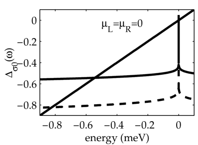
FIG. 1.: The graphical solution of the renormalization Eq. (5) for the spin $\uparrow$ (solid) and spin $\downarrow$ (dashed) level in the interacting region. The bare transition energy $\Delta^{0}_{\sigma 0}=-0.1$ relative to the chemical potential $\mu_{\alpha}=0$, the coupling strength $\Gamma_{\sigma}^{\alpha}=2\pi|v_{\sigma}|^{2}\rho_{\sigma}^{\alpha}=0.5$ and the temperature $kT=0.175$. The conduction band density of states $\rho_{\sigma}^{\alpha}=1/2W=1/100$. The spin polarization in the conduction band is given by the lower cut offs $-W_{\uparrow}^{\alpha}=-50,-W_{\downarrow}^{\alpha}=-12.5$ (units: meV).

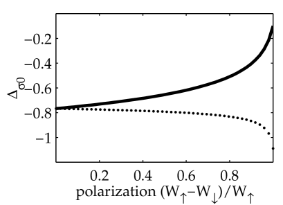
FIG. 2.: The dressed transition energies $\Delta_{\uparrow 0}$ (solid) and $\Delta_{\downarrow 0}$ (dashed) as a function of the spin polarization $(W_{\uparrow}^{\alpha}-W_{\downarrow}^{\alpha})/W_{\uparrow}^{\alpha}$ in the conduction bands. The polarization in the two leads are equal.

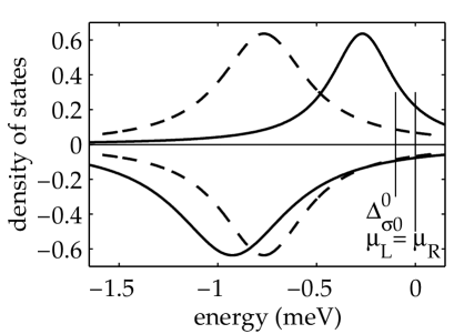
FIG. 3.: The equilibrium DOS of the interacting region for paramagnetically (dashed) and ferromagnetically (solid) ordered leads. In the ferromagnetically ordered case there is an amount of $3.5\%$ of the minority spin in the leads.

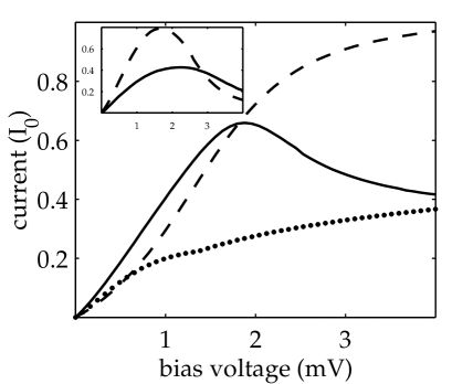
FIG. 4.: The tunneling current through the interacting region for paramagnetically (dashed) and ferromagnetically ordered leads. For the ferromagnetic ordering the minority spin percentage is 3.5 (solid) and 0 (dotted). The inset shows the situation where the conduction band width is $2W=2.8$ meV. $I_{0}=I^{\uparrow}_{0}+I^{\downarrow}_{0},\ I^{\sigma}_{0}=e\Gamma_{\sigma}/\hbar$.

REFERENCES

- [1] M. Johnson, Phys. Rev. B 58, 9635 (1998).
- [2] M. Julliere, Phys. Lett. 54A, 225 (1975).
- [3] J.S. Moodera, L.R. Kinder, T.M. Wong and R. Meservey, Phys. Rev. Lett. 74, 3273 (1995).
- [4] Y. Meir, N.S. Wingreen and P.A. Lee, Phys. Rev. Lett. 66, 3048 (1991); 70, 2601 (1993).
- [5] M. Pustilnik, Y. Avishai and K. Kikoin, Phys. Rev. Lett. 84, 1756 (2000).
- [6] D. Giuliano and A. Tagliacozzo. Phys. Rev. Lett. 84, 4677 (2000)
- [7] W.G. van der Wiel et al., Science, 289, 2105 (2000).
- [8] P. Recher, E.V. Sukhorukov, and D. Loss, Phys. Rev. Lett. 85, 1962 (2000).
- [9] A. Brataas, Y.V. Nazarov, and G.E.W. Bauer, Phys. Rev. Lett. 84, 2481 (2000).
- [10] B. Laikhtman, Phys. Rev. B, 41, 138 (1990); C.W.J. Beenakker, Phys. Rev. B, 44, 1646 (1991); A. Nakano R.K. Kalia, and P. Vashishta, Phys. Rev. B, 44, 8121 (1991); D. Goldhaber-Gordon et al., Nature (391), 156 (1998), Phys. Rev. Lett. 81, 5225 (1998); S.M. Cronenwett et al., Science (281), 540 (1998).
- [11] P.W. Anderson, Phys. Rev. 124, 41 (1961).
- [12] J. Hubbard, Proc. Roy. Soc. A 276, 238 (1963); 277, 237 (1963).
- [13] I. Sandalov and B. Johansson, Physica B 206-207, 712 (1995); I. Sandalov, B. Johansson and O. Eriksson, Physica B 259-261, 229 (1999); cond-mat/0011259.
- [14] J. Fransson, O. Eriksson, and I. Sandalov, in manuscript.
- [15] For example, such results were found for the Anderson model via summation of perturbation series [16] and via variational wave function for the total energy [17]. For the Hubbard model with an infinite Hubbard an expression similar to Eq. (5) was discovered by decoupling in terms of irreducible GF for Hubbard operators, Gutzwiller’s wave function and the three-body Faddeev equation [18, 19], via a Wick-like theorem for Hubbard operators [20] and for the -model [21].
- [16] A.F. Barabanov, K.A. Kikoin and L.A. Maksimov, Teor. Mat. Fiz 20, 364 (1974); 25, 87 (1975); Solid St. Comm. 15, 977 (1974); 18, 1527 (1976).
- [17] C.M. Varma and Y. Yafet, Phys. Rev. B 13, 2950 (1976).
- [18] L.D. Faddeev, Zh. Eksp. Teor. Fiz. 39, 1459 (1960) [Sov. Phys. JETP 12, 1014 (1961)].
- [19] A.E. Ruckenstein and S. Schmitt-Rink, Int. Journ. of Mod. Phys. B, 3, 1809 (1989).
- [20] Y.A. Izyumov, B.M. Letfulov, E.V. Shipitsyn and K.A. Chao, Int. Journ. Mod. Phys. B 6, 3479 (1992).
- [21] Y.A. Izyumov, B.M. Letfulov and E.V. Shipitsyn, J. Phys. Cond. Matter 6, 5137 (1994).
- [22] S. Hershfield, J.H. Davies and J.W. Wilkins, Phys. Rev. Lett. 67, 3720 (1991); Phys. Rev. B 46, 7046 (1992).
- [23] Y. Meir and N.S. Wingreen, Phys. Rev. Lett. 68, 2512 (1992).
- [24] N. Sivan and N.S. Wingreen, Phys. Rev. B, 54, 11622 (1996).
- [25] N. García, M. Muñoz, Y.-W. Zhao, Phys. Rev. Lett. 82, 2923 (1999).