Endogeneous Versus Exogeneous Shocks in Systems with Memory

Abstract

Systems with long-range persistence and memory are shown to exhibit different precursory as well as recovery patterns in response to shocks of exogeneous versus endogeneous origins. By endogeneous, we envision either fluctuations resulting from an underlying chaotic dynamics or from a stochastic forcing origin which may be external or be an effective coarse-grained description of the microscopic fluctuations. In this scenario, endogeneous shocks result from a kind of constructive interference of accumulated fluctuations whose impacts survive longer than the large shocks themselves. As a consequence, the recovery after an endogeneous shock is in general slower at early times and can be at long times either slower or faster than after an exogeneous perturbation. This offers the tantalizing possibility of distinguishing between an endogeneous versus exogeneous cause of a given shock, even when there is no “smoking gun.” This could help in investigating the exogeneous versus self-organized origins in problems such as the causes of major biological extinctions, of change of weather regimes and of the climate, in tracing the source of social upheaval and wars, and so on. Ref. [29] has already shown how this concept can be applied concretely to differentiate the effects on financial markets of the Sept. 11, 2001 attack or of the coup against Gorbachev on Aug., 19, 1991 (exogeneous) from financial crashes such as Oct. 1987 (endogeneous).

1 Introduction

Most complex systems around us exhibit rare and sudden transitions, that occur over time intervals that are short compared to the characteristic time scales of their posterior evolution. Such extreme events express more than anything else the underlying “forces” usually hidden by almost perfect balance and thus provide the potential for a better scientific understanding of complex systems. These crises have fundamental societal impacts and range from large natural catastrophes such as earthquakes, volcanic eruptions, hurricanes and tornadoes, landslides, avalanches, lightning strikes, meteorite/asteroid impacts, catastrophic events of environmental degradation, to the failure of engineering structures, crashes in the stock market, social unrest leading to large-scale strikes and upheaval, economic drawdowns on national and global scales, regional power blackouts, traffic gridlock, diseases and epidemics, and so on. It is essential to realize that the long-term behavior of these complex systems is often controlled in large part by these rare catastrophic events [25]. The outstanding scientific question is how such large-scale patterns of catastrophic nature might evolve from a series of interactions on the smallest and increasingly larger scales [28], or whether their origin should be searched from exogeneous sources.

Starting with Hurst’s study of 690 time series records of 75 geophysical phenomena, in particular river flow statistics, documenting the so-called “Hurst effect” of long term persistence [10], many studies in the last decades have investigated the existence of long memory effects in a large variety of systems, including meteorology (wind velocity, moisture transfer in the atmosphere, precipitation), oceanography (for instance wave-height), plasma turbulence, solar activity, stratosphere chemistry, seismic activity, internet traffic, financial price volatility, cardiac activity, immune response, and so on.

The question addressed here is whether the existence of long memory processes may lead to specific signatures in the precursory and in the relaxation/recovery/adaptation of a system after a large fluctuation of its activity, after a profound shock or even after a catastrophic event, that may allow one to distinguish an internal origin from an exogeneous source. Let us put this question in perspective with regards to the extinction of biological species as documented in the fossil record. During the past 550 million years, there have been purportedly five global mass extinctions, each of which had a profound effect on life on Earth. The last end-Cretaceous mass extinction (with the disappearance of $39-47\%$ of fossilizable genera and perhaps 75% of species) marking the Cretaceous/Tertiary (K/T) boundary about 65 millions ago is often attributed to the impact of a huge meteor in the Yucatan peninsula [15]. Another scenario is that a burst of active volcanism was the real origin of the extinction [4, 5]. It has been suggested that this extinction was actually driven by longer-term climatic changes, as evidence by the fact that certain species in the Late Maastrichtian disappeared a distinctive time before the K/T boundary [18, 19]. A completely endogeneous origin has also been proposed, based on the concepts of nonlinear feedbacks between species [20, 1] illustrated by self-organized criticality and punctuated equilibria [2, 24] (see [14] for a rebuttal). The situation is even murkier for the extinctions going further in the past, for which the smoking guns, if any, are not observable (see however the strong correlation between extinctions and volcanic traps presented in [5]). How can we distinguish between an exogeneous origin (meteorite, volcanism, abrupt climate change) and endogeneous dynamics, here defined as the progressive self-organizing response of the network of interacting species that may generate its own demise by nonlinear intermittent negative feedbacks or in response to the accumulation of slowly varying perturbations in the environment? Is it possible to distinguish two different exogeneous origins, one occurring over a very short time interval (meteorite) and the other extending over a long period of time (volcanism), based on the observations of the recovery and future evolution of diversity?

The aviation industry provides another vivid illustration of the question on the endogeneous versus exogeneous origin of a crisis. Recently, airlines became the prime industry victim of the September 11, 2001 terrorist attacks. The impact of the downturn in air travel has been severe not just on the airlines but also on lessors and aircraft manufacturers. The unprecedented drop in air travel and airline performance prompted the US government to provide $5 billion in compensation and to make available $10 billion in loan guarantees. This seems a clear-cut case for an exogeneous shock. However, the industry was deteriorating before the shock of September 11. In the first eight months of 2001, passenger traffic for US carriers rose by an anemic 0.7 percent, a sharp fall from annual growth of nearly 4 percent over the previous decade [3], illustrated by the record levels of the earned profits of $39 billion and of delivery of more than 4,700 jetliners from 1995 to 2000. The US airlines’ net profits dropped from margins of nearly 4 percent during 1998-2000 to losses of greater than 3 percent during the first half of 2001, despite aggressive price cuts as airlines tried to fill seats and profits vanished.

Many other examples are available. We propose to address this general question of exogeneous versus endogeneous origins of shocks by quantifying how the dynamics of the system may differ in its response to an exogeneous versus endogeneous shock. We start with a simple “mean field” model of the activity $A(t)$ of a system at time $t$, viewed as the effective response to all past perturbations embodied by some noisy function $\eta(\tau)$,

$$A(t)=\int_{-\infty}^{t}d\tau~{}\eta(\tau)~{}K(t-\tau)~{},$$ (1)

where $K(t-\tau)$ can be called the memory kernel, propagator, Green function, or response function of the system at a later time $t$ to a perturbation $\eta(\tau)$ that occurred at an earlier time $\tau$. Notwithstanding the linear structure of (1), we do not restrict our description to linear systems but take (1) as an effective coarse-grained description of possible complex nonlinear dynamics. For instance, it has been shown [30] that the extremal nonlinear dynamics of the Bak and Sneppen model and of the Sneppen model of extremal evolution of species, which exhibit a certain class of self-organized critical behavior [27], can be accurately characterized by the stochastic process called “Linear fractional stable motion,” which has exactly the form (1) for the activity dynamics.

Expression (1) contains for instance the fractional Brownian motion (fBm) model introduced by Mandelbrot and Van Ness [16] as a simple extension of the memoryless random walk to account for the Hurst effect. From an initial value $B_{H}(0)$, we recall that the fBm is defined by

$$B_{H}(t)-B_{H}(0)={1\over\Gamma(H+(1/2))}\int_{-\infty}^{t}d\tau~{}\eta(\tau)~{}K(t-\tau)~{},$$ (2)

where $d\tau~{}\eta(\tau)=dW_{\tau}$ is usually taken as the increment of the standard random walk with white noise spectrum and Gaussian distribution with variance ${\rm E}[dW_{\tau}]=d\tau$ and the memory kernel $K(t-\tau)$ is given by

$$K(t-\tau) = (t-\tau)^{H-{1\over 2}}~{},~{}~{}~{}~{}~{}{\rm for}~{}0\leq\tau\leq t$$ (3)

$$= (t-\tau)^{H-{1\over 2}}-(-\tau)^{H-{1\over 2}}~{},~{}~{}~{}~{}~{}~{}{\rm for}~{}\tau<0~{}.$$ (4)

For $H>1/2$, the fBm $B_{H}(t)$ exhibits long term persistence and memory, since the effect of past innovations of $dW_{\tau}$ is felt in the future with a slowly decaying power law weight $K(t-\tau)$. For our purpose, the fBm is non-stationary and it is more relevant to consider globally statistically stationary processes.

Here, we consider processes which can be described by an integral equation of the form (1) and (2) but with possibly different forms for the noise innovations $\eta$ and for the memory kernel $K$. Simple viscous systems correspond to $K(t-\tau)\propto\exp[-(t-\tau)/T]$, where $T$ is a characteristic relaxation time. Complex fluids, glasses, porous media, semiconductors, and so on, are characterized by a memory kernel $K(t-\tau)\propto e^{-a(t-\tau)^{\beta}}$, with $0<\beta<1$, a law known under the name Kohlrausch–Williams–Watts law [23]. It is also interesting to consider fractional noise motion (fNm) defined as the time derivative of $B_{H}(t)$, which does possess the property of statistical stationarity. A fNm is defined by (1) with

$$K_{\rm fNm}(t-\tau)={1\over(t-\tau)^{{3\over 2}-H}}={1\over(t-\tau)^{1-\theta}}~{},$$ (5)

for $H=1/2+\theta$. Persistence $1/2<H<1$ (respectively antipersistence $0<H<1/2$) corresponds to $0<\theta<1/2$ (respectively $-1/2<\theta<0$). Such a memory kernel describes also the renormalized Omori’s law for earthquake aftershocks [26, 8].

2 Exogeneous versus endogeneous shock

In the following, we consider systems described by a long memory integral (1) with kernel $K(t)$ decaying faster than $1/\sqrt{t}$ at large times, so as to ensure the condition of statistical stationarity. This excludes the fBm which are non-stationary processes but includes the fNm.

2.1 Exogeneous shock

An external shock occurring at $t=0$ can be modeled in this framework by an innovation which takes the form of a jump $A_{0}~{}\delta(\tau)$. The response of the system for $t>0$ is then

$$A(t)=A_{0}~{}K(t)+\int_{-\infty}^{t}d\tau~{}\eta(\tau)~{}K(t-\tau).$$ (6)

The expectation of the response to an exogeneous shock is thus

$${\rm E}_{\rm exo}[A(t)]=A_{0}~{}K(t)+n\langle\eta\rangle~{},$$ (7)

where $\langle\eta\rangle$ is the average noise level and $n=\int_{0}^{+\infty}d\tau~{}K(\tau)$ is the average impact of a perturbation which is usually smaller than $1$ to ensure stationarity (this corresponds to the sub-critical regime of branching processes [7]).

The time evolution of the system after the shock is thus the sum of the process it would have followed in absence of shock and of the kernel $K(t)$. The response $A_{0}~{}K(t)$ to the jump $A_{0}~{}\delta(\tau)$ examplifies that $K(t)$ is the Green function or propagator of the coarse-grained equation of motions of the system. Expression (6) simply expresses that the recovery of the system to an external shock is entirely controled by its relaxation kernel.

2.2 Endogeneous shock

2.2.1 Conditional response function

Let us consider the natural evolution of the system, without any large external shock, which nevertheless exhibits a large burst $A(t=0)=A_{0}$ at $t=0$. From the definition (1), it is clear that a large “endogeneous” shock requires a special set of realization of the innovations $\{\eta(t)\}$. To quantify the response in such case, we recall a standard result of stochastic processes with finite variance and covariance that the expectation of some process $X(t)$ conditioned on some variable $Y$ taking a specific value $Y_{0}$ is given by [11]

$${\rm E}[X(t)|Y=A_{0}]-{\rm E}[X(t)]=\left(A_{0}-{\rm E}[Y]\right)~{}{{\rm Cov}(X(t),Y)\over{\rm E}[Y^{2}]}~{},$$ (8)

where ${\rm E}[Y^{2}]$ denotes the expectation of $Y^{2}$, ${\rm Cov}(X(t),Y)$ is the covariance of $X$ and $Y$, ${\rm E}[X(t)]$ and ${\rm E}[Y]$ are the (unconditional) average of $X(t)$ and of $Y$. Expression (8) recovers the obvious result that ${\rm E}[X(t)|Y=A_{0}]={\rm E}[X(t)]$ if $X$ and $Y$ are uncorrelated. A result generalizing (8) holds when $\eta(\tau)$ has an infinite variance corresponding to a distribution with a power law tail with exponent smaller than $2$ [9].

Let us assume that the process $A(t)$ and the innovations $\eta$’s have been defined with zero mean, which is always possible without loss of generality by a translation. Let us call $X(t>0)=A(t)$ and $Y=A(0)$. Under the assumption that the noise $\eta(\tau)$ has a finite variance, we obtain from (1)

$${\rm Cov}(A(t),A(0))=\int_{-\infty}^{0}d\tau~{}K(t-\tau)~{}K(-\tau)~{},$$ (9)

and

$${\rm E}[A(0)^{2}]=\int_{-\infty}^{0}d\tau~{}[K(-\tau)]^{2}~{}.$$ (10)

For stationary processes such that $K(t)$ decays faster than $1/\sqrt{t}$ so as to make the integral in (10) convergent, ${\rm E}[A(0)^{2}]$ is a constant. We thus obtain the posterior ($t>0$) response (above the stationary average) to an endogenous shock occurring at time $t=0$ under the form of a conditional expectation of $A(t)$, conditioned by the existence of this shock:

$${\rm E}_{\rm endo}[A(t)|A(0)=A_{0}]\propto A_{0}\int_{0}^{+\infty}du~{}K(t+u)~{}K(u)~{},$$ (11)

for large $A_{0}$. This relaxation of the activity after an endogeneous shock is in general significantly different from that given by (7) following an exogeneous shock.

2.2.2 Conditional noise trajectory

What is the source of endogeneous shocks characterized by the response function (11)? To answer, let us consider the process $W(t)\equiv\int_{-\infty}^{t}d\tau~{}{\hat{\eta}}(\tau)$, where ${\hat{\eta}}(t)=\eta(t)-\langle\eta\rangle$ defines the centered innovations forcing the system (1). Using the property (8), we find that for $t<0$

$${\rm E}_{\rm endo}[W(t)|A(0)=A_{0}]=\frac{{\rm Cov}[W(t),A(0)]}{{\rm Var}[A(0)]}\cdot\left(A_{0}-{\rm E}[A]\right)\propto\left(A_{0}-{\rm E}[A]\right)\int_{-\infty}^{t}d\tau~{}K(-\tau)~{},$$ (12)

where ${\rm E}_{\rm endo}[W(t)|A(0)=A_{0}]=0$ for $t>0$ since the conditioning does not act after the shock. Expression (12) predicts that the expected path of the continuous innovation flow prior to the endogeneous shock (i.e., for $t<0$) grows like $\Delta W(t)={\hat{\eta}}(t)\Delta t\sim K(-t)\Delta t$ upon the approach to the time $t=0$ of the large endogeneous shock. In other words, conditioned on the observation of a large endogeneous shock, there is specific set of trajectories of the innovation flow $\eta(t)$ that led to it. These conditional innovation flows have an expectation given by (12).

Inserting the expression (12) for the average conditional noise in the definition (1) of the process, we obtain an expression proportional to (11). This shows that the precursory activity preceding and announcing the endogeneous shock follows the same time dependence as the relaxation (11) following the shock, with the only modification that $t$ (for $t>0$ counting time after the shock at $t=0$) is changed into $-t$ (for $t<0$ counting time before the shock at $t=0$). We can also use (12) into (1) and calculate the activity after the endogeneous shock to recover (11). These are two equivalent ways of arriving at the same result, the one using (12) illuminating the fundamental physical origin of the endogeneous response.

These results allow us to understand the distinctive features of an endogeneous shock compared to an external shock. The later is a single very strong instantaneous perturbation that is sufficient in itself to move the system significantly according to (6). In contrast, an “endogeneous” shock is the result of the cumulative effect of many small perturbations, each one looking relatively benign taken alone but, when taken all together collectively along the full path of innovations, can add up coherently due to the long-range memory of the dynamical process. In summing, the term “endogeneous” is used here to refer to the sum of the contribution of many “small” innovations adding up according to a specific most probable trajectory, as opposed to the effect of a single massive external perturbation.

2.3 Numerical simulation of an epidemic branching process with long-range memory

To illustrate our predictions (7) and (11), we use a simple epidemic branching model defined as follows. The model describes the time evolution of the rate of occurrence of events as a function of all past history. What is called “event” can be the creation of a new species or a new family of organisms as in [6], the occurrence of an earthquake as in [26, 8], the amplitude of the so-called financial volatility as in [29] or of aviation traffic, a change of weather regime, a climate shift and so on. The rate $\lambda(t)$ of events at time $t$ is assumed to be a function of all past events according to

$$\lambda(t)=\sum_{i~{}|~{}t_{i}<t}~{}\phi(t-t_{i})~{},$$ (13)

where the sum is carried over all past events that occurred at times $t_{i}$ prior to the present $t$. The influence of such an event at a previous time $t_{i}$ is felt at time $t$ through the bare propagator $\phi(t-t_{i})$. In our present illustration, we consider a process equivalent to a fNm with Hurst exponent $H=1/2+\theta$, which can be shown to correspond to the choice $\phi(t)=\theta~{}c^{\theta}/(t+c)^{1+\theta}$, where $c$ is an ultra-violet regularization time embodying a delay process at early times in the activity response after an event. Indeed, the Master equation corresponding to the process (13) can be shown [26, 8] to be nothing but (1) with the renormalized or dressed propagator $K(t)\propto 1/(t+c)^{1-\theta}$.

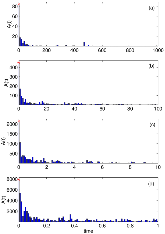
Figure 1: Rate of activity following an exogeneous shock in a numerical simulation of the epidemic branching model (13) generated with a memory kernel decaying as a power law $\phi(t)\sim 1/(t+c)^{1+\theta}$ with parameters $\theta=0.1$ and $c=0.001$ without a constant source term ($\mu=0$). The rate of activity following an exogeneous shock that occurred at $t=0$ is shown at increasing magnification from top to bottom. It is evaluated using a bin size decreasing by factors of $10$ from $\delta t=10$ (a) to $\delta t=0.01$ (d). Averaging over many such realizations would yield the average power law decay $K(t)\sim 1/(t+c)^{1-\theta}$ predicted by (7).

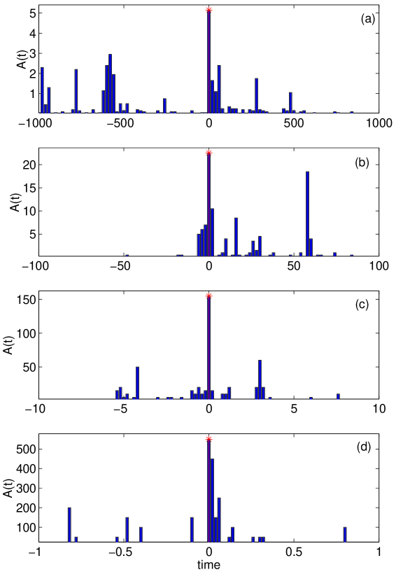
Figure 2: Rate of activity prior to and after an endogeneously generated major burst of activity generated by a numerical simulation of the epidemic branching model (13) with a power law kernel with the same parameters $\theta=0.1$ and $c=0.001$ as in figure 1 with in addition a constant Poisson source term with rate $\mu=0.001$ corresponding, on average, to one event added from an external source per $1000$ time units. Most of the observed activity is thus the result of interactions between events. The rate of activity close to the largest peak of activity is shown at increasing magnifications from top to bottom and is evaluated as in figure 1. Both precursory and relaxational processes can be observed at many time scales.

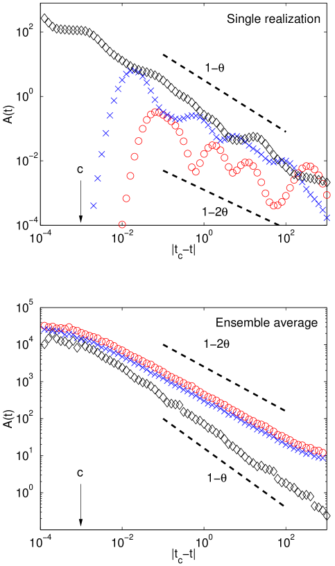
Figure 3: Rate of activity for a single sequence (a) of the epidemic branching model defined by (13) generated with a memory kernel decaying as a power law of time with the parameters $\theta=0.2$ and $c=10^{-3}$ and averaged over many sequences (b). The exogeneous relaxation is shown with diamonds, the endogeneous relaxation is shown as crosses and circles are for the precursory activity in the endogeneous case. Large fluctuations are observed in the precursory activity and in the endogeneous relaxation when looking at a single sequence, due to the small number $\approx 100$ of observed events. Averaging over 50 realizations, we see clearly the faster decay rate $\sim 1/t^{1-\theta}$ for the exogeneous relaxation predicted by (7) compared with the endogenous one predicted by (11). The same decay rate $\sim 1/t^{1-2\theta}$ predicted by (11) is observed for both the endogeneous precursory and post-event relaxation.

Numerical simulations of the epidemic branching process are performed by drawing events in succession according to a non-stationary Poisson process with instantaneous rate (13). Figures 1 and 2 show successive magnifications of time series of the activity rate after an exogeneous shock and around an endogeneous shock, respectively, in order to visualize the precursory and relaxation activities. In figure 2, an external source of activity necessary for seeding has been added as a Poisson process of rate $\mu=10^{-3}$ corresponding on average to one external event over a time interval of $1000$. The most striking visual difference is the existence of the precursory signal occurring at many time scales for the endogeneous shock. Figure 3 quantifies the precursory and relaxation rates associated with activity shocks. The top panel shows the relaxation of the activity (rate of events) following an external shock compared to that after an endogeneous shock, for a single realization. $t_{c}$ is the time of the shock. The horizontal axis is $t-t_{c}$ for the relaxation of the activity after the shock. The precursory activity prior to the shock is also shown for the endogeneous shock as a function of $t_{c}-t$. The bottom panel shows the same three activity functions after averaging over many realizations, translating time in the averaging so that all shocks occur at the same time denoted $t_{c}$. The prediction (7) states that the relaxation of the activity after an exogeneous shock should decay as $K(t)\propto 1/(t-t_{c}+c)^{1-\theta}$ while the decay after an endogeneous shock should be given by (11) which predicts the law $\propto 1/(t-t_{c}+c)^{1-2\theta}$, that is, a significantly smaller exponent for $\theta>0$. Similarly, we predict that the precursory activity prior to an endogeneous shock should increase as $\propto 1/(t_{c}-t+c)^{1-2\theta}$. These predictions are verified with very good accuracy, as seen in figure 3.

These simulations confirm that there is a distinctive difference in the relaxation after an endogeneous shock compared to an exogeneous shock, if the memory kernel is sufficiently long-ranged. For a single realization, there are unavoidable fluctuations that may blur out this difference. However, we see a quite visible precursory signal (foreshock activity) that is symmetric to that relaxation process in the case of an endogeneous shock. This follows from the model used here which obeys the time-reversal symmetry. This may be used as a distinguishing signature of an endogeneous shock.

3 Classification of the distinctive responses for different classes of memory kernels

The family of power law kernels used in the simulations presented in figures 1, 2 and 3 are only one possibility among many. Our formalism allows us to classify the distinctive properties of the relaxation and precursory behaviors that can be expected for an arbitrary memory kernel. We now provide this classification by studying (7) and (11).

3.1 Short-time response

We compare the initial slopes of the relaxations after the occurrence of the shock at $t=0$. Thus, by short-time, we mean the asymptotic decay law just after the shock. For this, we expand (7) to get

$${\rm E}_{\rm exo}[A(t)]=A_{0}~{}K(0)\left[1+{K^{\prime}(0)\over K(0)}~{}~{}t+{\cal O}(t^{2})\right]=A_{0}~{}K(0)\left[1+{d\ln K\over dt}|_{t=0}~{}~{}t+{\cal O}(t^{2})\right]~{},$$ (14)

where $K^{\prime}(t)$ denotes the derivative of $K(t)$ with respect to time.

Similarly, expanding the integral in (11) for short times, we obtain

$${\rm E}_{\rm endo}[A(t)|A(0)=A_{0}]\propto A_{0}F(0)\left[1+{1\over 2}{d\ln F\over dt}|_{t=0}~{}~{}t+{\cal O}(t^{2})\right]~{},$$ (15)

where

$$F(t)\equiv\int_{t}^{+\infty}du[K(u)]^{2}~{}$$ (16)

is a monotonically decreasing function of time.

It is convenient to use the parameterization

$$F(t)=e^{-g(t)}~{},$$ (17)

where $g(t)$ is an monotonously increasing function of time. Inserting (17) in (14) and (15) leads to

$${\rm E}_{\rm exo}[A(t)]=A_{0}~{}K(0)\left[1-\left({1\over 2}g^{\prime}(0)-{1\over 2}{g^{\prime\prime}(0)\over g^{\prime}(0)}\right)~{}t+{\cal O}(t^{2})\right]~{},$$ (18)

and

$${\rm E}_{\rm endo}[A(t)|A(0)=A_{0}]\propto A_{0}F(0)\left[1-{1\over 2}g^{\prime}(0)~{}t+{\cal O}(t^{2})\right]~{}.$$ (19)

1. For $g^{\prime\prime}(0)=0$, that is, $g(t)=2\alpha t$ corresponding to an pure exponential relaxation $K(t)\propto\exp[-\alpha t]$, the velocities of the responses to an exogeneous and to endogeneous shock are identical;

2. for $g^{\prime\prime}(0)>0$ corresponding to a super-exponential relaxation $K(t)\propto\exp[-\alpha t^{c}]$ with $c>1$, the exogeneous relaxation is slower than the endogeneous one;

3. for $g^{\prime\prime}(0)<0$ corresponding to a sub-exponential relaxation such as a stretched exponential $K(t)\propto\exp[-\alpha t^{c}]$ with $c<1$ or to the family of regularly varying functions such as power laws, the exogeneous relaxation is faster than the endogeneous one.

The exponential relaxation thus marks the boundary between two opposite regimes. As is intuitive, a sub-exponential relaxation betraying a long memory process leads to a slower short-time recovery after an endogeneous shock, because it results from a long preparation process (12).

3.2 Asymptotic long-time response

Since $K(t)$ is a monotonously decaying function, $K(t+u)\leq K(t)$ for any $u\geq 0$. This leads to the following inequality

$${\rm E}_{\rm endo}[A(t)|A(0)=A_{0}]\leq A_{0}K(t)\int_{0}^{+\infty}du~{}K(u)~{},$$ (20)

which is valid if the integral $\int_{0}^{+\infty}du~{}K(u)$ exists, that is, if $K(t)$ decays faster than $1/t$ at large times. This shows that, as soon as $K(t)\ll C/t$ for any positive constant $C$, ${\rm E}_{\rm endo}[A(t)|A(0)=A_{0}]<{\rm E}_{\rm exo}[A(t)]$. But the difference may be small and inobservable. For instance, for $K(t)\propto 1/t^{1+\theta}$ with $\theta>0$, a careful examination of the integral in (11) shows that, due to the contribution of the conditional noise close to the shock, we have

$${\rm E}_{\rm endo}[A(t)|A(0)=A_{0}]\propto{A_{0}\over t^{1+\theta}}\sim{\rm E}_{\rm exo}[A(t)]~{}.$$ (21)

Thus, there is no qualitative difference in the relaxation rates of an endogeneous shock and exogeneous shock in this case: the contributions of all the conditional activity prior to the endogeneous shock is equivalent to that of the shock itself. A more elaborate and analysis specific to the problem at hand must be performed to predict the prefactors that will be different in the endogeneous and exogeneous cases.

In constrast, for memory kernels $K(t)\propto 1/t^{1-\theta}$ with $\theta>0$ decaying slower than $1/t$, as for a stationary fNm of the form (5), we obtain

$${\rm E}_{\rm endo}[A(t)|A(0)=A_{0}]\propto{A_{0}\over t^{1-2\theta}}\gg{\rm E}_{\rm exo}[A(t)]\propto{A_{0}\over t^{1-\theta}}~{}.$$ (22)

In this case, the relaxation following an endogeneous shock decays significantly more slowly than for an exogeneous shock. This case is examplified in figure 3. In the long time limit, the decay law $1/t$ thus marks the boundary between two opposite regimes.

3.3 Illustration

An illustration of this critical behavior is provided by the response of the price volatility $\sigma_{{\Delta t}}$ at scale ${\Delta t}$ defined as the amplitude (absolute value) of the return $r_{Dt}(t)\equiv\ln[p(t)/p(t-{\Delta t})]=\epsilon(t)\cdot\sigma_{{\Delta t}}(t)=\epsilon(t)\cdot e^{{\omega}_{{\Delta t}}(t)}$. of a financial asset. $\epsilon(t)$ is a random sign. Indeed, financial price time series have been shown to exhibit a long-range correlation of their log-volatility ${\omega}_{{\Delta t}}$, described by a model [22, 29] in which ${\omega}_{{\Delta t}}(t)$ follows the process (1) with

$$K_{\Delta t}(t)\sim K_{0}\sqrt{\frac{\lambda^{2}T}{t}}~{}~{}~{}~{}{\rm for}~{}~{}{\Delta t}\ll t\ll T~{},$$ (23)

where $T\approx 1$ year is a so-called integral time scale. This form (23) corresponds to the parameterization (5) with $\theta=1/2$. Sornette et al. [29] have shown that there is a clear distinction between the relaxation of stock market volatility after an exogeneous event such at the September 11, 2001 attack or the Aug., 19, 1991 coup against Gorbachev and that after an endogeneous event such as the October 19, 1987 crash. In this model, the long-range memory acting on the logarithm of the volatility induces an additional effect, namely the exponent of the power law relaxation after an endogeneous shock is a linear function of the amplitude of the shock.

3.4 Synthesis of the asymptotic short- and long-time regimes

We have found two special functional forms for the response kernel $K(t)\propto 1/t$ and $K(t)\propto\exp[-\alpha t]$, which are “invariant” or indifferent with respect to the endogeneous versus exogeneous origin of a shock. Thus, for normal exponential relaxation processes as well as for power relaxation $\propto 1/t$, the functional form of the recovery does not allow one to distinguish between an endogeneous and an exogeneous shock.

These two invariants $K(t)\propto\exp[-\alpha t]$ and $K(t)\propto 1/t$ delineate two opposite regimes, the first one for short-time scales and the second one for long-time scales:

1. for $K(t)\propto 1/t^{1-\theta}$ with $\theta>0$, the endogeneous response decays more slowly than the exogeneous response, at all time scales;

2. for $\exp[-\alpha t]\ll K(t)\ll 1/t$ for any positive $\alpha$, the endogeneous response decays more slowly than the exogeneous response at short time scales and has the same dependence as the exogeneous response at long time scales; this regime describes for instance the stretched exponential relaxation of complex fluids alluded to above;

3. for $K(t)\ll\exp[-\alpha t]$ for any positive $\alpha$, the endogeneous response decay faster than the exogeneous response at all time scales.

More complicated behaviors can occur when the memory kernel $K(t)$ exhibits a change of regime, crossing the exponential and/or $1/t$ boundaries at certain time scales. Each situation requires a specific analysis which yields sometimes surprising non-intuitive results [9].

4 Conclusion

We think that the conceptual framework presented here may be applied to a large variety of situations, beyond those alluded to in the introduction. For instance, the result (12) has been shown to explain the so-called inverse Omori’s law for earthquake foreshock activity before a mainshock, in a simple model of earthquake triggering [9]. The same mechanism may explain the premonitory seismicity pattern known as “burst of aftershocks” [13]: a mainshock with an abnormally large number of aftershocks has been found to be a statistically significant precursor to strong earthquakes [21].

Many dynamical systems in Nature, such as geophysical and biological systems (immune network, memory processes in the brain, etc.), or created by man such as social structures and networks (Internet), States and so on, exhibit long-memory effects due to a wealth of possible mechanisms. For instance, Krishan Khurana at UCLA has suggested to us that the concept proposed here could explain that endogeneous civil wars have long-lasting effects with slow reconstruction compared with the fast recovery after exogeneous wars (that is, imposed or coming from the outside). The increasing emphasis on the concepts of emergence and complexity has emphasized an endogeneous origin of the complicated dynamical behavior of complex systems. In reality, most (so-called) complex systems are the result of their internal dynamics/adaptation in response to a flow of external perturbations, but some of these external perturbations are rare extreme shocks. What is the role of these exogeneous shocks in the self-organization of a complex system? Can one distinguish the impact of extreme exogeneous shocks from an endogeneous organization at different time scales? Our present analysis has just scratched the surface of these important and deep questions by suggesting an angle of attack based on the conditional historical process at the basis of strong endogeneous fluctuations. Extensions of the present simplified framework involve the generalization to multidimensional coupled processes such as in [12] and to nonlinear spatio-temporal processes.

We are grateful to A.B. Davis. V. Keilis-Borok and V.F. Pisarenko for useful exchanges. This work was partially supported by the James S. Mc Donnell Foundation 21st century scientist award/studying complex system.

References

- [1] Allen, J.C., W.M. Schaffer and D. Rosko, Chaos reduces species extinction by amplifying local population noise, Nature 364, 229-232, 1993.
- [2] Bak, P., How nature works: the science of self-organized criticality, New York, NY, USA : Copernicus, 1996.
- [3] Costa, P., D.S. Harned and J.T. Lundquist, Rethinking the aviation industry, McKinsey Quarterly 2, Risk and resilience, 2002,
- [4] Courtillot, V.E., A volcanic eruption, Scientific American 263 N4:85-92, 1990.
- [5] Courtillot, V.E., Evolutionary catastrophes: the science of mass extinction, New York: Cambridge University Press, 1999.
- [6] Courtillot, V. and Y. Gaudemer, Effects of mass extinctions on biodiversity, Nature 381, 146-148, 1996.
- [7] Harris, T.E., The theory of branching processes, Springer, Berlin, 1963.
- [8] Helmstetter, A. and D. Sornette, Sub-critical and Super-critical Regimes in Epidemic Models of Earthquake Aftershocks, in press in J. Geophys. Res. (e-print at http://arXiv.org/abs/cond-mat/0109318)
- [9] Helmstetter, A., D. Sornette, J.-R. Grasso, Mainshocks are Aftershocks of Conditional Foreshocks: How do foreshock statistical properties emerge from aftershock laws, submitted to J. Geophys. Res. (http://arXiv.org/abs/cond-mat/0205499)
- [10] Hurst, H.E., Long term storage capacity of reservoirs, Transactions of the American Society of Civil Engineers, 116, 770-808, 1951.
- [11] Jacod, J. and A. N. Shiryaev, Limit Theorems for Stochastic Processes, Springer, Berlin, 1987.
- [12] Jefferies, P., Lamper, D. and Johnson, N.F., Anatomy of extreme events in a complex adaptative system, e-print at cond-mat/0201540
- [13] Keilis-Borok, V.I., I.M. Rotwain and T.V. Sidorenko, Intensified sequence of aftershocks as a precursor of strong earthquake, Dokl. Akad. Nauk. SSSR, 242(3), 567-569, 1978.
- [14] Kirchner, J.W. and Weil, A., No fractals in fossil extinction statistics, Nature 395 N6700, 337-338, 1998.
- [15] Kyte, F.T., A meteorite from the Cretaceous/Tertiary boundary, Nature, 396 N6708:237-239 (1998).
- [16] Mandelbrot, B.B. and J.W. Van Ness, Fractional Brownian motions, fractional noise and applications, Society for Industrial and Applied Mathematics Review, 10, 422-437, 1968.
- [17] Mandelbrot, B.B. and J.R. Wallis, Noah, Joseph and operational hydrology, Water Resources Research, 4, 909-918, 1968.
- [18] Marshall, C.R. Palaeobiology - Mass extinction probed, Nature 392 N6671:17-19 (1998).
- [19] Marshall, C.R. and P.D. Ward, Sudden and gradual extinctions in the lastest Cretaceous of Western European Tethus, Science 274 N5291:1360-1363 (1996).
- [20] Milton, J.G. and J. Belair, Chaos, noise and extinction in models of population growth, Theor. Population Biol. 37, 273-290, 1990.
- [21] Molchan, G.M., O.E. Dmitrieva, I.M. Rotwain and J. Dewey, Statistical analysis of the results of earthquake prediction, based on bursts of aftershocks, Phys. Earth and Planetary Interiors 61, 128-139, 1990.
- [22] Muzy, J.F., J. Delour and E. Bacry, Modelling fluctuations of financial time series: from cascade process to stochastic volatility model, The European physical Journal B 17, 537-548 (2000).
- [23] Phillips, J.C., Stretched exponential relaxation in molecular and electronic glasses, Rep. Prog. Phys. 59, 1133-1208, 1996.
- [24] Sole, R.V., Manrubia, S.C., Benton, M. and Bak, P., Self-similarity of extinction statistics in the fossil record, Nature 388 N6644:764-767 (1997).
- [25] Sornette, D., Complexity, catastrophe and physics, Physics World 12 (N12), 57-57, 1999.
- [26] Sornette, A. and D. Sornette, Renormalization of earthquake aftershocks, Geophys. Res. Lett., 26, 1981-1984, 1999.
- [27] Sornette, D., Critical Phenomena in Natural Sciences, Springer Series in Synergetics, Heidelberg, 2000.
- [28] Sornette, D., Predictability of catastrophic events: material rupture, earthquakes, turbulence, financial crashes and human birth, Proc. Nat. Acad. Sci. USA 99 SUPP1, 2522-2529, 2002.
- [29] Sornette, D., Y. Malevergne and and J.F. Muzy, Volatility fingerprints of large shocks: Endogeneous versus exogeneous, Risk Magazine (2002) (http://arXiv.org/abs/cond-mat/0204626)
- [30] Krishnamurthy, S., Tanguy, A., Abry, P. and Roux, S., A stochastic description of extremal dynamics, Europhysics Lett. 51, 1-7 (2000).