Statistical dynamical mean-field description of strongly correlated disordered electron-phonon systems

Abstract

Combining the self-consistent theory of localization and the dynamical mean-field theory, we present a theoretical approach capable of describing both self-trapping of charge carriers during the process of polaron formation and disorder-induced Anderson localization. By constructing random samples for the local density of states (LDOS) we analyze the distribution function for this quantity and demonstrate that the typical rather than the mean LDOS is a natural measure to distinguish between itinerant and localized states. Significant polaron effects on the mobility edge are found.

71.38.-k, 72.10.Di, 71.35.Aa The question of how the electron-phonon (EP) interaction influences the localization transition caused by disorder [1], i.e. by strong impurity-induced spatial fluctuations in the potential energy, has been addressed by Anderson about thirty years ago [2]. He called attention to the particular importance of EP coupling effects in the vicinity of the so-called ”mobility edge”, separating itinerant (extended) and localized states. Nevertheless, there is as yet not much theoretical work even for the simplest case of a single electron moving in a disordered, deformable medium.

As a first step towards addressing this problem, in Ref. [3] the single-particle Holstein model with site-diagonal, binary-alloy-type disorder was studied within the dynamical mean field approximation (DMFA) [4]. The DMFA, however, cannot (fully) discriminate between itinerant and localized states, mainly because the randomness is treated at the level of the coherent potential approximation. In order to remedy this shortcoming, recently the authors [5] adopted the statistical DMFA (statDMFA) [6] to the Anderson-Holstein Hamiltonian,

$${\cal H}=\sum_{i}\epsilon_{i}n_{i}-J\sum_{\langle ij\rangle}(c_{i}^{\dagger}c_{j}+{\rm H.c.})-\sqrt{E_{p}\Omega}\sum_{i}(b_{i}+b_{i}^{\dagger})n_{i}+\Omega\sum_{i}b_{i}^{\dagger}b_{i}\,,$$ (1)

where $J$ denotes the electron transfer amplitude, $\Omega$ is the frequency of the optical phonon, $E_{p}$ is the polaron shift, and the on-site energies $\{\epsilon_{i}\}$ are assumed to be independent random variables with probability density $p(\epsilon_{i})=(1/\gamma)\theta(\gamma/2-|\epsilon_{i}|)$. The statDMFA is essentially a probabilistic method (in the sense of the self-consistent theory of localization [7]), based on the construction of random samples for the physical quantities of interest.

As a natural measure of the itinerancy of a polaron state, we consider the tunneling rate from a given site, defined - on a Bethe lattice with connectivity $K$ ($\tilde{J}=J\sqrt{K}$) - as the imaginary part of the hybridization function

$$\Gamma_{i}(\omega)=(\pi\tilde{J}^{2}/K)\sum_{l=1}^{K}N_{l}(\omega),\quad\mbox{where}\quad N_{l}(\omega)=-(1/\pi){\rm Im}{\cal G}_{l}(\omega)$$ (2)

is the local density of states (LDOS). The LDOS, directly connected to the local amplitude of the electron wave function, undergoes a qualitative change upon localization implying a vanishing tunneling rate $\Gamma_{i}(\omega)$ for a localized state at energy $\omega$. The local single-particle Green function and the related hybridization function are given by ($z=\omega+i\eta$)

$${\cal G}_{i}(z)={1\over z-\epsilon_{i}-H_{i}(z)-{\Sigma}_{i}(z)}\quad\mbox{and}\quad H_{i}={{\tilde{J}^{2}}\over K}\sum_{l=1}^{K+1}{1\over{z-\epsilon_{l}-\bar{H}_{l}^{i}-\bar{\Sigma}_{l}^{i}}},$$ (3)

respectively. We now ignore that the functions on the rhs of $H_{i}$ should be calculated for the Bethe lattice with the site $i$ removed, i.e. we make the replacement $\{\bar{\cal G}_{l}^{i},\;\bar{H}_{l}^{i},\;\bar{\Sigma}_{l}^{i}\}\;\leadsto\;\{{\cal G}_{l},\;H_{l},\;\Sigma_{l}\}$, and furthermore take $K$ as the typical number of terms even for the central site. Finally, the EP self-energy contribution is determined in the limit $K\to\infty$. The self-energy is then local and, in terms of a continuous fraction expansion, takes the form

$$\Sigma_{l}(z)=\frac{E_{p}1\Omega}{[F_{l}^{(1)}(z)]^{-1}-\frac{E_{p}2\Omega}{[F_{l}^{(2)}(z)]^{-1}-...}},$$ (4)

with $[F_{l}^{(p)}(z)]^{-1}=z-p\Omega-\epsilon_{i}-H_{l}^{(p)}(z)$ and $H_{l}^{(p)}(z)=H_{l}(z-p\Omega$). Here the energy shift keeps track of the number of virtual phonons ($0\!<\!p\!<\!M$). Regardless of the local EP self-energy, the statDMFA takes spatial fluctuations of, e.g., the LDOS into account and provides an adequate description of disorder effects. Due to the randomness in the on-site energies, the tunneling rate and consequently the LDOS is a random variable, and the question of whether it vanishes or not depends on the probability density exhibiting different features for itinerant and localized states [1, 7]. In particular, the difference between the mean and typical LDOS,

$${N}^{\rm mean}(\omega)=\frac{1}{N}\sum_{i}^{N}N_{i}(\omega)\quad\mbox{and}\quad N^{\rm typ}(\omega)=\exp\left[\frac{1}{N}\sum_{i}^{N}\log N_{i}(\omega)\right]$$ (5)

obtained by the arithmetic and geometric mean of the LDOS, respectively, is a useful measure to discriminate between extended and localized states. ${N}^{\rm mean}(\omega)>0$ but $N^{\rm typ}(\omega)=0$ indicates a localized state at energy $\omega$.

In the numerical work, we calculated the LDOS by solving a recursion scheme for $H_{l}^{(p)}$ which depends on $K\varepsilon_{j}^{\;\prime}\mbox{s}$, $KH_{j}^{(p)\;\prime}\mbox{s}$, $\ldots$, and $KH_{j}^{(p_{max})\;\prime}\mbox{s}$. Starting from an initial random configuration for the independent variables  $H_{l}^{(p)}$, which is successively updated with a sampling technique similar to the one described in Ref. [7], we constructed self-consistent random samples for $H_{l}^{(p)}$, using $K=2$, $N=100\,000$, $M=35$, and $\eta=10^{-8}$.

Without disorder, the physical properties of the Holstein model are determined by two interaction parameters, $\tilde{\lambda}=E_{p}/2\tilde{J}$ and $g^{2}=E_{p}/\Omega$, and the adiabaticity ratio $\tilde{\alpha}=\Omega/\tilde{J}$. Polaron formation sets in provided that $\tilde{\lambda}\gtrsim 1/\sqrt{K}$ and $g^{2}\gtrsim 1$. Of course, the internal structure of the polaron depends on $\tilde{\alpha}$.

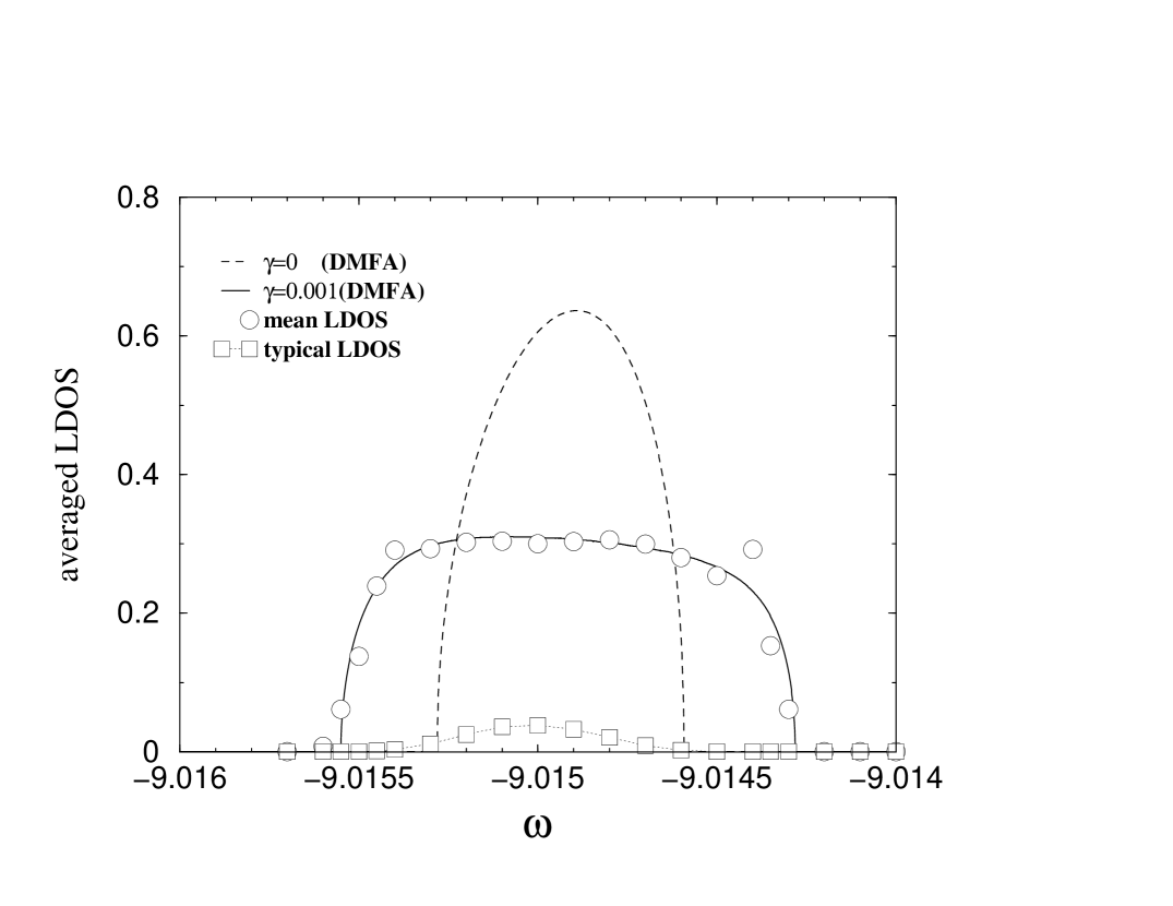
Figure 1: Mean and typical LDOS for the lowest polaron subband in the non-adiabatic strong EP coupling region ($\tilde{\lambda}=9.0$, $\tilde{\alpha}=2.25$, and $J=0.5$). The pronounced disorder-induced broadening of the LDOS occurs because the variation of the on-site energies $\gamma=0.001$ is on the order of the strongly renormalized band width $\tilde{W}$.

Disorder affects polaron states quite differently in the adiabatic ($\tilde{\alpha}\ll 1$), non-adiabatic ($\tilde{\alpha}\sim 1$), and antiadiabatic ($\tilde{\alpha}\gg 1$) cases. Without EP coupling, i.e. in the pure Anderson model, the critical disorder strength needed to localize all states is $(\gamma_{c}/\tilde{W}_{0})_{\rm complete}\approx 2.25$, where $\tilde{W}_{0}=4\tilde{J}$. In the weak EP coupling regime, it has been shown that the quantum interference needed for localization is significantly suppressed by inelastic polaron-phonon scattering processes [5]: States above the optical phonon emission threshold are more difficult to localize than the corresponding bare electron states. In the very strong EP coupling regime, extremely weak disorder turns itinerant into localized polaron states. Surprisingly, the ratio $(\gamma_{c}/\tilde{W})_{\rm complete}$, where $\tilde{W}$ is the band width of the lowest polaron subband, is almost the same as for a bare electron. In fact, in the non-adiabatic strong EP coupling regime, where the band collapse changes only the overall energy scale, disorder affects a polaron in a similar way as a bare electron. For example, the LDOS and mobility edges are symmetric (cf. Fig. 1).

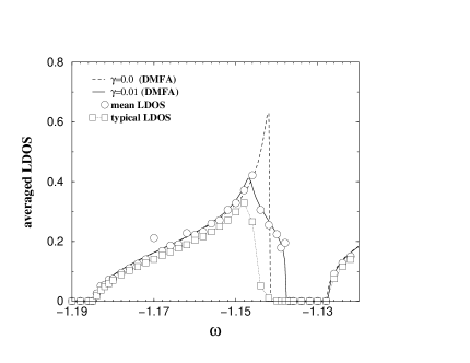
Figure 2: Left panel: Mean and typical LDOS in the adiabatic intermediate-to-strong EP coupling region ($\tilde{\lambda}=1.0$, $\tilde{\alpha}=0.25$, $J=0.5$). Note that $N^{\rm mean}(\omega)$ is almost perfectly approximated by the DMFA. At about $\omega=-1.13$ the second polaronic subband starts. Right panel: Probability density of the LDOS for four representative energies $\omega$. The inset shows the probability distribution, i.e., the cumulant of the probability density.

In the adiabatic intermediate-to-strong EP coupling regime the physics is much more involved. Here the band dispersion of the lowest subband significantly deviates from a rescaled bare band [8], leading to a strong asymmetric LDOS. Specifically, the states at the bottom of the subband are mostly electronic and rather mobile due to long-range tunneling induced by EP coupling, whereas the states at the top of the subband are rather phononic and immobile [8]. As a direct consequence, the states at the zone boundary are very susceptible to disorder, i.e. the critical disorder strength needed to localize these states is much smaller than for states at the bottom, and, from the results for the typical LDOS, we find asymmetric mobility edges (see Fig. 2). Moreover, $(\gamma_{c}/\tilde{W})_{\rm complete}\approx 2.8$, which is larger than the corresponding ratio for a bare electron. Thus, contrary to naive expectations, at intermediate EP couplings, an adiabatic polaron is even more difficult to localize than a bare electron.

It is very instructive to discuss the behaviour of the probability density of the LDOS and the corresponding probability distribution. Note that both quantities have to be calculated self-consistently within our sampling procedure. The right panel of Fig. 2 shows the dramatic change of the probability density of $N_{l}(\omega)$ when the system undergoes the localization transition by crossing the mobility edge. In the region of localized states, the probability density for the LDOS is broad and very asymmetric and, as a consequence, the mean LDOS is not representative.

In conclusion, in terms of the Anderson Holstein model, we have demonstrated that the statDMFA, which according to the spirit of Anderson’s early work [1] focuses on distribution functions and associates typical rather than mean values to physical quantities, yields a proper description of disordered electron-phonon systems.

References

- [1] P. W. Anderson, Phys. Rev. 109, 1498 (1958).
- [2] P. W. Anderson, Nature Phys. Science 235, 163 (1972)
- [3] F.X. Bronold, A. Saxena, and A. R. Bishop, Phys. Rev. B 63, 235109 (2001).
- [4] A. Georges et al., Rev. Mod. Phys. 68, 13 (1996).
- [5] F.X. Bronold and H. Fehske, Phys. Rev. B, accepted for publication (2002).
- [6] V. Dobrosavljević and G. Kotliar, Phys. Rev. Lett. 78, 3943 (1997).
- [7] R. Abou-Chacra, P. W. Anderson, and D. Thouless, J. Phys. C 6, 1734 (1973).
- [8] H. Fehske, J. Loos, and G. Wellein, Z. Phys. B 104, 616 (1997).