Ground state of a double-exchange system containing impurities: bounds of ferromagnetism

Abstract

We study the boundary between ferromagnetic and non-ferromagnetic ground state of a double-exchange system with quenched disorder for arbitrary relation between Hund exchange coupling and electron band width. The boundary is found both from the solution of the Dynamical Mean Field Approximation equations and from the comparison of the energies of the saturated ferromagnetic and paramagnetic states. Both methods give very similar results. To explain the disappearance of ferromagnetism in part of the parameter space we derive from the double-exchange Hamiltonian with classical localized spins in the limit of large but finite Hund exchange coupling the $t-J$ model (with classical localized spins).

I Introduction

The problem of ferromagnetism in the double-exchange (DE) model [1, 2, 3], which appears due to the Hund exchange coupling between the core spins and the mobile carriers, has a long history (see Ref. [4] and references therein). Frequently the modeling deals with the case of infinite Hund exchange. In this approximation the ground state of the system is always ferromagnetic (FM). To describe possible non-FM ground states of such a system one has to introduce direct antiferromagnetic exchange between the core spins. However, the finite Hund exchange by itself generates effective antiferromagnetic exchange, thus destroying ferromagnetism in a part of the system parameter space.

In our previous publication [5] on the basis of DMFA we obtained the closed formula for the ferromagnet-paramagnet (FM-PM) transition temperature $T_{c}$ for the double-exchange system for arbitrary relation between Hund exchange coupling and electron band width. In this paper we present a detailed study of of the boundary between FM and non-FM ground state of the system found from that formula, and, independently, from comparison of energies of the saturated FM and PM states. In addition, from the double-exchange Hamiltonian with classical localized spins in the limit of large but finite Hund exchange coupling we obtain the classical version of the $t-J$ model.

II Hamiltonian and DMFA equations

Consider the DE model with random on-site energies. The Hamiltonian of the model is

$$H=\sum_{nn^{\prime}\alpha}t_{n-n^{\prime}}c_{n\alpha}^{\dagger}c_{n\alpha}+\sum_{n\alpha}V_{n}c_{n\alpha}^{\dagger}c_{n\alpha}$$ (1)

$$-J\sum_{n\alpha\beta}{\bf m}_{n}\cdot{\bf\sigma}_{\alpha\beta}c_{n\alpha}^{\dagger}c_{n\beta},$$ (2)

where $t_{n-n^{\prime}}$ is the electron hopping, $J$ is the effective exchange coupling between a core spin and a conduction electron, $\hat{\bf\sigma}$ is the vector of the Pauli matrices, and $\alpha,\beta$ are spin indices. We express the localized (classical) spin by ${\bf m}_{n}=(m_{n}{}^{x},m_{n}{}^{y},m_{n}{}^{z})$ with the normalization $|{\bf m}|^{2}=1$. To take into account the chemical disorder introduced by doping impurities, which is generic for the manganites and many other DE systems, we consider the case random on-site energy $V_{n}$.

In a single electron representation the Hamiltonian can be presented as

$$H_{nn^{\prime}}=H^{0}_{n-n^{\prime}}+\left(V_{n}-J{\bf m}_{n}\cdot{\bf\sigma}\right)\delta_{nn^{\prime}};$$ (3)

the first is translationaly invariant, the second describes quenched disorder, and the third - annealed disorder.

The DMFA, as applied to the problem under consideration, is based on two assumptions. The first assumption is that the averaged, with respect to random orientation of localized spins and random on-site energy $V$, locator

$$\hat{G}_{\rm loc}(z)=\left\langle\hat{G}_{nn}(z)\right\rangle_{{\bf m},V},$$ (4)

where

$$\hat{G}(z)=(z-H)^{-1},$$ (5)

can be expressed through the the local self-energy $\hat{\Sigma}$ by the equation

$$\hat{G}_{\rm loc}(z)=g_{0}\left(z-\hat{\Sigma}(z)\right),$$ (6)

where

$$g_{0}(z)=\frac{1}{N}\sum_{\bf k}\left(z-H^{0}_{\bf k}\right)^{-1}$$ (7)

is the bare (in the absence of the disorder and exchange interaction) locator. Thus introduced self-energy satisfies equation

$$\hat{G}_{\rm loc}(z)=\left\langle\frac{1}{\hat{G}_{\rm loc}^{-1}(z)+\hat{\Sigma}(z)-V_{n}+J{\bf m}\cdot\hat{\bf\sigma}}\right\rangle_{{\bf m},V}.$$ (8)

The system of equations (6) and (8) is very much similar to the well known CPA equations (see [6] and references therein), as generalized to the case when the quantities $\hat{G},\hat{\Sigma}$ and $\hat{g}$ are $2\times 2$ matrices in spin space [7]. The system of equations however, is not yet closed. The averaging with respect to annealed disorder is principally different from the averaging with respect to quenched disorder.

The second assumption of the DMFA is the prescription for the determining, in our case, the probability of a spin configuration self-consistently with the solutions of the Eqs. (6) and (8). To formulate the DMFA equation for this probability, taking into account both kinds of the disorder, let us start from the general formula for the partition function

$${\cal Z}_{V_{n}}=\int\exp\left(-{\rm Tr}\sum_{s}\log\hat{G}(z_{s})\right)\prod_{n}d{\bf m}_{n},$$ (9)

where $z_{s}=i\omega_{s}+\mu$; $\omega_{s}$ is the Matsubara frequency and $\mu$ is the chemical potential. The averaging over $\left\{{\bf m}_{n}\right\}$ is given by

$$\left\langle\Phi\right\rangle_{\bf m}=\frac{1}{{\cal Z}_{V}}\int\exp\left(-{\rm Tr}\sum_{s}\log\hat{G}(z_{s})\right)\Phi({\bf m})\prod_{n}d{\bf m}_{n}.$$ (10)

All observables, in particular thermodynamic potential $\Omega$, should additionally be averaged over the realizations of the quenched disorder; in particular

$$\Omega=-\frac{1}{\beta}\left\langle\log{\cal Z}_{V}\right\rangle_{{\bf m},V}.$$ (11)

The DMFA approximates the multi-spin probability ${\cal Z}_{V}^{-1}\exp\left(-{\rm Tr}\log\hat{G}\right)$ as a product of one-site probabilities in such a way, that

$$\frac{\delta\Omega}{\delta\hat{G}_{\rm loc}}=0.$$ (12)

The result for the one-site probability reads (for details of the calculation see Ref. [8]):

$$P_{V_{n}}({\bf m})\propto\exp\left[-\beta\Delta\Omega_{{\bf m},V_{n}}\right],$$ (13)

where

$$\Delta\Omega_{{\bf m},V_{n}}=-\frac{1}{\beta}\sum_{s}{\rm Tr}\log\left[1+\hat{G}_{\rm loc}(z_{s})\right.$$ (14)

$$\left.\left(J{\bf m}\cdot\hat{\bf\sigma}-V_{n}+\hat{\Sigma}(z_{s})\right)\right]e^{i\omega_{s}0_{+}}.$$ (15)

is the change of the thermodynamic potential of the electron gas described by the Green’s function $\hat{G}_{\rm loc}$ due to interaction with a single impurity [9, 10].

The right hand side of Eq. (13), is a complicated non-linear functional of $P_{V}({\bf m})$. However, if we are interested only in the transition temperature $T_{c}$, the problem can be reduced to a traditional mean field (MF) equation. In linear with respect to magnetization $M$ approximation Eq. (13) takes the form

$$P_{V_{n}}({\bf m})\propto\exp\left(-\beta I_{V_{n}}{\bf M}\cdot{\bf m}\right).$$ (16)

Non-trivial solution of the MF equation

$${\bf M}=\int\left\langle P_{V_{n}}({\bf m})\right\rangle_{V}{\bf m}d{\bf m}.$$ (17)

can exist only for $T<T_{\rm c}$, where $T_{c}=\frac{1}{3}\left\langle I_{V_{n}}\right\rangle_{V}$.

III $T_{\rm c}$ for the semi-circular DOS

For simplicity consider the semi-circular (SC) bare density of states (DOS) $N_{0}(\varepsilon)$, the bandwidth being $2W$. Then

$$g_{0}(z)=\int\frac{N_{0}(\varepsilon)d\varepsilon}{z-\varepsilon}=\frac{2}{W}\left[\frac{z}{W}-\sqrt{\left(\frac{z}{W}\right)^{2}-1}\right].$$ (18)

For this case

$$\hat{\Sigma}=z-2w\hat{G}_{\rm loc}-\hat{G}_{\rm loc}^{-1},$$ (19)

where $w=W^{2}/8$. Thus from Eqs. (6) and (8) we obtain a single equation for $\hat{G}_{\rm loc}$

$$\hat{G}_{\rm loc}(z)=\left\langle\frac{1}{z-2w\hat{G}_{\rm loc}(z)-V_{n}+J{\bf m}\cdot\hat{\bf\sigma}}\right\rangle_{{\bf m},V},$$ (20)

and Eq. (14) can be presented as

$$\Delta\Omega_{{\bf m},V_{n}}=\frac{1}{\beta}\sum_{s}\log\det\left[z_{s}-2w\hat{G}_{\rm loc}(z_{s})\right.$$ (21)

$$\left.-V_{n}+J{\bf m}\cdot\hat{\bf\sigma}\right]e^{i\omega_{s}0_{+}}.$$ (22)

In linear with respect to $M$ approximation

$$\hat{G}_{\rm loc}=g\hat{I}-hJ{\bf M\cdot\hat{\sigma}},$$ (23)

where $g$ is locator in paramagnetic phase, given by the equation

$$g=\frac{1}{2}\left[\left\langle\frac{1}{z-2wg-V_{n}-J}\right\rangle_{V}\right.$$ (24)

$$\left.+\left\langle\frac{1}{z-2wg-V_{n}+J}\right\rangle_{V}\right],$$ (25)

and the quantity $h$ is given by the formula

$$h=\frac{\left\langle\Delta_{V_{n}}\right\rangle_{V}}{1-\frac{4J^{2}w}{3}\left\langle\Delta_{V_{n}}^{2}\right\rangle_{V}-2w\left\langle\Delta_{V_{n}}\right\rangle_{V}},$$ (26)

where

$$\Delta_{V_{n}}(z_{s})=\frac{1}{\left[z_{s}-2wg(z_{s})-V_{n}\right]^{2}-J^{2}}.$$ (27)

Expanding Eq. (21) we obtain the effective exchange integral is

$$I_{V_{n}}=\frac{4J^{2}w}{\beta}\sum_{s}h(z_{s})\Delta_{V_{n}}(z_{s}).$$ (28)

If we transform the sum over the imaginary Matsubara frequencies in the right-hand side of Eq. (28) to integral over real energies $E$, we obtain for the $T_{\rm c}$

$$T_{\rm c}=\frac{4J^{2}w}{3\pi}\int_{-\infty}^{\infty}f(E)\mbox{Im}\left[h(E_{+})\left\langle\Delta_{V_{n}}(E_{+})\right\rangle_{V}\right]dE,$$ (29)

where $f(E)$ is the Fermi function, and $E_{+}=E+i0$. To the best of our knowledge this closed formula which takes into account both finite value of Hund exchange and quenched disorder was obtained and studied by us for the first time [5]. According to this formula the boundary between the FM and non-FM ground states is found from equating $T_{c}$ to zero, which reads

$$\int_{-\infty}^{E_{F}^{(p)}}\mbox{Im}\left[h(E_{+})\left\langle\Delta_{V_{n}}(E_{+})\right\rangle_{V}\right]dE=0;$$ (30)

the Fermi energy $E_{F}^{(p)}$ is found from the equation

$$n=-\frac{2}{\pi}\int_{-\infty}^{E_{F}^{(p)}}{\rm Im}\;g(E_{+})\;dE,$$ (31)

where $n$ is the number of electrons per site.

Thus found $T_{c}$ is the temperature at which the paramagnetic state became unstable with respect to small spontaneous magnetic moment. This becomes especially obvious, if we obtain the equation for the $T_{c}$ by constructing Landau functional [8]. Independently, one may consider another approach to the same problem based on the comparison of the energies of the saturated FM state and PM state. The energy of the PM state is found from the equation

$$E_{p}=-\frac{2}{\pi}\int_{-\infty}^{E_{F}^{(p)}}E\;{\rm Im}\;g(E_{+})\;dE;$$ (32)

the energy of the saturated FM state and the appropriate Fermi energy are found from the equations:

$$E_{f}=-\frac{1}{\pi}\int_{-\infty}^{E_{F}^{(f)}}E\;[{\rm Im}\;g_{\uparrow}(E_{+})+{\rm Im}\;g_{\downarrow}(E_{+})]\;dE$$ (33)

$$n=-\frac{1}{\pi}\int_{-\infty}^{E_{F}^{(f)}}{\rm Im}\;[{\rm Im}\;g_{\uparrow}(E_{+})+{\rm Im}\;g_{\downarrow}(E_{+})]dE,$$ (34)

where the FM locator $g_{\uparrow\downarrow}$ is given by the equation.

$$g_{\uparrow\downarrow}=\left\langle\frac{1}{z-2wg-V_{n}\mp J}\right\rangle_{V}.$$ (35)

The boundary of the ferromagnetic region at the phase diagram can be found from the equality between the two energies: $E_{p}=E_{f}$. We thus use an alternative to the second assumption of the DMFA.

IV FM – non-FM boundary

The boundary of the FM ground state of the system in case of no quenched disorder is presented on Fig. 1.

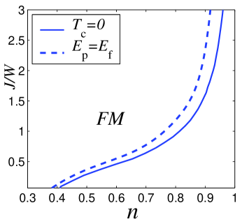
FIG. 1.: The FM – non-FM boundary for the case of no quenched disorder in the coordinates of relative strength of the Hund exchange $J/W$ and electron concentration $n$.

The diagram agrees with those obtained on the basis of numerical calculations [11] and from qualitative reasoning [10].

To consider the influence of chemical disorder we consider the model in which $V_{n}=V$ with the probability $x$, and $V_{n}=0$ with the probability $1-x$, thus $x$ being the concentration of impurities. In this model we consider the number of electrons $n$ and the concentration of impurities $x$ as two independent parameters. Solving equation for the locator we obtain the boundaries which are presented on Figs. 2-4. It is interesting that ferromagnetism is now precluded in much larger region of the $J/W-n$ plane.

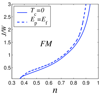
FIG. 2.: The FM – non-FM boundary for $V/W=.5$ and $x=.3$ in the coordinates of relative strength of the Hund exchange $J/W$ and electron concentration $n$.

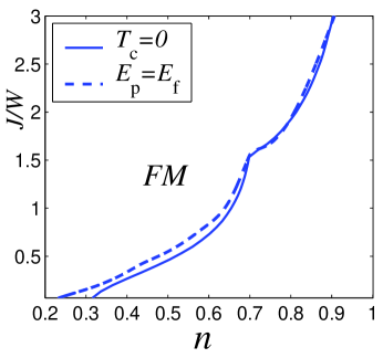
FIG. 3.: The FM – non-FM boundary for $V/W=1$ and $x=.3$ in the coordinates of relative strength of the Hund exchange $J/W$ and electron concentration $n$.

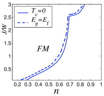
FIG. 4.: The FM – non-FM boundary for $V/W=2$ and $x=.3$ in the coordinates of relative strength of the Hund exchange $J/W$ and electron concentration $n$.

The boundaries between the phases make sharp bends for static disorder strong enough to create a gap between conduction and impurity bands both in ferromagnetic and paramagnetic phases [12]. In this case the number of states in the impurity band is equal to the concentration of impurities, and for $n=1-x$ the Fermi energy is in the gap. To emphasize this fact we plot the density of states both for FM and PM phases at the values of parameters $V/W$, $x$ and $J/W$ which correspond to the sharp bends on Figs. 3 and 4.

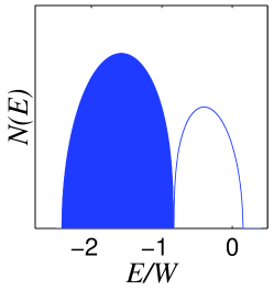
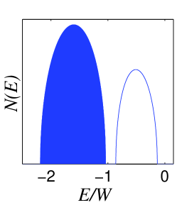
FIG. 5.: Density of states for $V/W=1$, $x=.3$, $J/W=1.53$ for saturated FM phase (left) and PM phase (right); occupied states for $n=0.7$ are filed.

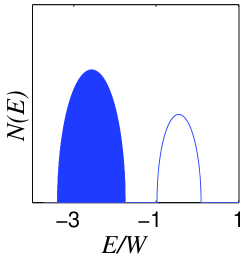
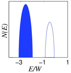
FIG. 6.: Density of states for $V/W=2$, $x=.3$, $J/W=2.53$ for saturated FM phase (left) and PM phase (right); occupied states for $n=0.7$ are filed.

A From the double-exchange Hamiltonian to the $t-J$ model: Classical spins

The Hamiltonian of the DE model [1, 2, 3] is

$$H=-J_{H}\sum_{n\alpha\beta}{\bf m}_{n}\cdot{\bf\sigma}_{\alpha\beta}c_{n\alpha}^{\dagger}c_{n\beta}-\sum_{nn^{\prime}\alpha}t_{nn^{\prime}}c_{n\alpha}^{\dagger}c_{n^{\prime}\alpha},$$ (A1)

where $t_{n-n^{\prime}}$ is the electron hopping, $J_{H}$ is the effective Hund exchange coupling between a core spin and a conduction electron, $\hat{\bf\sigma}$ is the vector of the Pauli matrices, and $\alpha,\beta$ are spin indices. We express the localized (classical) spin by a unit vector whose orientation is determined by polar angle $\theta$ and azimuthal angle $\phi$. In a single electron representation the Hamiltonian can be presented as

$$H_{nn^{\prime}}=H^{ex}+H^{kin}=-J_{H}{\bf m}_{n}\cdot{\bf\sigma}\delta_{nn^{\prime}}-t_{nn^{\prime}}.$$ (A2)

We consider the case of strong exchange: $J_{H}\gg W$ where $W$ is the electron band width. In this case we should first diagonalize the exchange part of the Hamiltonian. This is done by choosing local spin quantization axis on each site in the direction of ${\bf m}$. In this representation the Hamiltonian is [13]

$$H_{nn^{\prime}}=-J_{H}\sigma^{z}\delta_{nn^{\prime}}-t_{nn^{\prime}}\left(\begin{array}[]{cc}a_{nn^{\prime}}&b_{nn^{\prime}}\\ b_{n^{\prime}n}^{*}&a_{n^{\prime}n}\end{array}\right),$$ (A5)

where

$$a_{nn^{\prime}}=\cos\frac{\theta_{n}}{2}\cos\frac{\theta_{n^{\prime}}}{2}+\sin\frac{\theta_{n}}{2}\sin\frac{\theta_{n^{\prime}}}{2}e^{i(\phi_{n^{\prime}}-\phi_{n})}$$ (A6)

$$b_{nn^{\prime}}=\sin\frac{\theta_{n}}{2}\cos\frac{\theta_{n^{\prime}}}{2}e^{-i\phi_{n}}-\cos\frac{\theta_{n}}{2}\sin\frac{\theta_{n^{\prime}}}{2}e^{-i\phi_{n^{\prime}}}.$$ (A7)

The transformation to local spin quantization axis including an additional Euler rotation angle, which leads to a more involved effective Hamiltonian than A5, was introduced by Nagaev [14].

The next step, like it is done in the derivation of the $t-J$ model from the Hubbard model [15], is to apply a canonical transformation

$$H\rightarrow\tilde{H}=e^{S}He^{-S}=H+[S,H]+\frac{1}{2}[S[S,H]]+\dots$$ (A8)

which excludes all band-to-band transitions. This can be achieved if we chose the operator $S$ in the form

$$S_{nn^{\prime}}=\frac{t_{nn^{\prime}}}{2J_{H}}\left(\begin{array}[]{cc}a_{nn^{\prime}}&b_{nn^{\prime}}\\ -b_{n^{\prime}n}^{*}&a_{n^{\prime}n}\end{array}\right).$$ (A11)

We have

$$[S,H^{ex}]_{nn^{\prime}}=t_{nn^{\prime}}\left(\begin{array}[]{cc}0&b_{nn^{\prime}}\\ b_{n^{\prime}n}^{*}&0\end{array}\right)$$ (A14)

$$\left[S,[S,H^{ex}]\right]_{nn}=2\sum_{n^{\prime\prime}}J_{nn^{\prime\prime}}\left(\begin{array}[]{cc}-|b_{nn^{\prime\prime}}|^{2}&0\\ 0&|b_{nn^{\prime\prime}}|^{2}\end{array}\right),$$ (A17)

where $J_{nn^{\prime\prime}}=|t_{nn^{\prime\prime}}|^{2}/(2J_{H})$. Keeping terms up to the second order with respect to $t$ (and only site-diagonal part of the second order terms) we obtain

$$\tilde{H}_{nn^{\prime}}=-J_{H}\sigma^{z}\delta_{nn^{\prime}}-t_{nn^{\prime}}\left(\begin{array}[]{cc}a_{nn^{\prime}}&0\\ 0&a_{n^{\prime}n}\end{array}\right)$$ (A20)

$$+\sum_{n^{\prime\prime}}J_{nn^{\prime\prime}}({\bf m}_{n}\cdot{\bf m}_{n^{\prime\prime}}-1)\sigma^{z}\delta_{nn^{\prime}},$$ (A21)

In the second quantization form the Hamiltonian (A20) has the form (ignoring the constant term)

$$\tilde{H}=-\sum_{nn^{\prime}}t_{nn^{\prime}}a_{n^{\prime}n}d_{n}^{\dagger}d_{n^{\prime}}$$ (A22)

$$+\sum_{nn^{\prime}}J_{nn^{\prime}}{\bf m}_{n}\cdot{\bf m}_{n^{\prime}}(1-d_{n}^{\dagger}d_{n}),$$ (A23)

where for the case of hole doping $d^{\dagger}(d)$ is the operator of creation (annihilation) of the hole, and for the case of electron doping it is the operator of creation (annihilation) of the electron.

Looking at the Hamiltonian obtained, we see that large but finite Hund exchange dynamically generates antiferromagnetic exchange (the second term in Eq. (A22). This term, however, is not independent upon the electron (hole) subsystem. In this regard this Heisenberg like term resembles the first non-Heisenbergian term (kinetic exchange).

This research was supported by the Israeli Science Foundation administered by the Israel Academy of Sciences and Humanities and BSF.

REFERENCES

- [1] C. Zener, Phys. Rev. 82, 403 (1951).
- [2] P. W. Anderson and H. Hasegawa, Phys. Rev. 100, 675 (1955).
- [3] P. G. De Gennes, Phys. Rev. 118, 141 (1960).
- [4] N. Furukawa: in Physics of Manganites, ed. T. Kaplan and S. Mahanti (Plenum Publishing, New York, 1999).
- [5] M. Auslender and E. Kogan, EuroPhys. Lett. (2002).
- [6] J. M. Ziman, Models of Disorder (Cambridge University Press, Cambridge, 1979).
- [7] A. Rangette, A. Yanase, and J. Kubler, Solid State Comm. 12, 171 (1973); K. Kubo, J. Phys. Soc. Japan 36, 32 (1974).
- [8] M. Auslender and E. Kogan, Phys. Rev. B65, 012408 (2002); Physica A 302, 345 (2001).
- [9] S. Doniach and E. H. Sondheimer, Green’s functions for solid state physicists (Imperial College Press, London, 1998).
- [10] A. Chattopadhyay, A. J. Millis, S. Das Sarma, Phys. Rev. B61, 10738 (2000).
- [11] E. Dagotto, S. Yunoki, A. L. Malvezzi, A. Moreo, J. Hu, S. Capponi, D. Poilblanc, and N. Furukawa, Phys. Rev. B58, 6414 (1998).
- [12] M. Auslender and E. Kogan, Eur. Phys. J. B, 19, 525 (2001).
- [13] E. M. Kogan and M. I. Auslender, phys. stat. sol. (b) 147, 613 (1988).
- [14] E.L. Nagaev, Physics of magnetic semiconductors, p. 116 (Mir Publishers, Moscow, 1983);
- [15] Yu. A. Izyumov, Physics-Uspekhi, 40, 445 (1997). .