Binary tree summation Monte Carlo simulation for Potts models

Abstract

In this talk, we briefly comment on Sweeny and Gliozzi methods, cluster Monte Carlo method, and recent transition matrix Monte Carlo for Potts models. We mostly concentrate on a new algorithm known as ‘binary tree summation’. Some of the most interesting features of this method will be highlighted – such as simulating fractional number of Potts states, as well as offering the partition function and thermodynamic quantities as functions of temperature in a single run.

1 Introduction

The Potts model [1] is not only fascinating in relation to phase transitions but also an excellent model for constructing new algorithms for Monte Carlo simulation. Before the advent of cluster algorithms, Sweeny [2] in 1983 already had an algorithm that has much reduced critical slowing down. Sweeny algorithm is a heat-bath algorithm in the Fortuin-Kasteleyn representation [3] of the Potts model as a percolation problem for any positive real value of the number of Potts state $q$. Any thermodynamic averages in the Potts model representation can be translated into a percolation bond representation [4]. Sweeny algorithm can be efficiently implemented only in two dimensions. In three and higher dimensions, it becomes too expensive to simulate, because each move requires a step to identify if two sites belong to the same or different clusters. Nevertheless, it is perhaps the only algorithm that works for any real values of $q$.

Very recently, Gliozzi [5] introduced a set of different transition probabilities than that of Sweeny’s. In Gliozzi’s rate, those links that are occupied by bonds or pair of unoccupied sites that connect the same cluster are resampled with probability $p$ for occupation, and $1-p$ for empty. For unoccupied sites that belong to two different clusters, the probability for occupation by a bond is $p/q$ and empty $1-p/q$. The resampling of a large fraction of the links appears to decorrelate the configuration efficiently. Gliozzi claims [5] that his algorithm does not suffer from critical slowing down. We have shown by explicit calculation of the correlation times that this is not true [6]. In two dimensions, we have good logarithmic divergence of the correlation time with system linear sizes for the Ising model. For two-dimensional three-state Potts model, we found dynamical critical exponent $z\approx 0.5$, and for the three-dimensional Ising model, the exponent is about 0.4.

The Swendsen-Wang [7] and Wolff [8] algorithms work only for integer values of $q$. They can be implemented very efficiently. For the Swendsen-Wang algorithm, each sweep takes CPU time of $O(N)$, and for Wolff algorithm, it is proportional to the size of the cluster that is being flipped. They reduce but not completely eliminate critical slowing down at the critical temperature.

The traditional methods mentioned above simulate at one fixed temperature $T$, thus the results are in terms of discrete points. A curve is obtained by connecting these points. The transition matrix Monte Carlo [9] and other related algorithms [10, 11, 12, 13] generate continuous function of temperature or other variable from a single simulation, thus greatly enhanced efficiency. The multi-histogram sampling of Weigel et al [14] in the context of $q$-state Potts model should be mentioned here. The multicanonical simulation method of Berg [11, 15] also has the additional advantage of much reduced correlation times for first-order phase transitions.

It is very attractive to have algorithms that do not have correlation at all. In fact, there are such algorithms, such as that of random percolation. Since the samples are drawn at random for each configuration, each configuration is independent of the previous configurations. The simple sampling method of Hu [16] has this property. Newman and Ziff [17] gave an efficient implement that work by exact weighting of the probability $p$ so that after the simulation, the whole curve $Q$ of some physical observable versus $p$ can be computed. In this paper, we present some attempts [18] that generalize Newman-Ziff method to general Potts model of $q$ states. These algorithms all have the common feature that bonds are added to the system one by one. Once there are on the lattice, they do not move. It is a nonequilibrium process in the sense that there is no (Monte Carlo) time translation invariance for the process. The rest of the paper is organized as follows: in the next section, we briefly review the Newman-Ziff method, followed by generalization of the partition function to Potts model. We then discuss a number of algorithms, and show their efficiencies and also point out their shortcomings. We conclude in the last section.

2 Newman-Ziff-type methods

Consider the simple bond percolation problem. We generate configurations by putting bonds at every nearest neighbor link of a $d$-dimensional hypercubic lattice with probability $p$, and absence of bond with probability $1-p$. Any average of physical quantity $Q(\Gamma)$ of configuration $\Gamma$ can be computed exactly from

$$\langle Q\rangle=\sum_{\Gamma}Q(\Gamma)p^{b}(1-p)^{M-b},$$ (1)

where the summation is over all the $2^{M}$ configurations; $b$ is number of bonds present, and $M=Nd$ is maximum possible number of bonds.

In a standard simulation, one fixes a value of $p$, and generates configurations by visiting each link and putting a bond with probability $p$. Estimates of $\langle Q\rangle$ are obtained by taking sample means of quantity $Q(\Gamma)$. Newman and Ziff [17] instead considered a computation of $Q_{b}$ for each value of $b$, and then reconstructed from $Q_{b}$ the function $\langle Q\rangle$ of $p$. From Eq. (1), we have

$$\langle Q\rangle=\sum_{b=0}^{M}\sum_{\Gamma_{b}}Q(\Gamma_{b})p^{b}(1-p)^{M-b}=\sum_{b=0}^{M}p^{b}(1-p)^{M-b}{M!\over b!(M-b)!}Q_{b},$$ (2)

where $Q_{b}$ is defined as average over all the $M!/(b!(M-b)!)$ configurations $\Gamma_{b}$ of exactly $b$ number of bonds,

$$Q_{b}={b!(M-b)!\over M!}\sum_{\Gamma_{b}}Q(\Gamma_{b}).$$ (3)

Newman and Ziff proposed the following algorithm to evaluate $Q_{b}$. Each sweep of the lattice starts with empty lattice, putting bonds one by one at random over these that is empty. This will generate $M+1$ configurations with 0, 1, $\cdots$, $b$, $\cdots$, $M$ number of bonds. From them, we calculate $Q_{b}$ for each $b$. With the help of Hoshen-Kopelman algorithm [19], the whole calculation of one sweep can be done in CPU time of $O(N)$. Although configurations within a sweep are highly correlated, each sweep is an independent one. Very accurate percolation threshold was obtained this way.

To generalize this procedure to Potts model, we note that the analogous equation to Eq. (2) is

$$\langle Q\rangle=\sum_{b=0}^{M}\sum_{\Gamma_{b}}Q(\Gamma_{b})p^{b}(1-p)^{M-b}q^{N_{c}(\Gamma_{b})}=\sum_{b=0}^{M}p^{b}(1-p)^{M-b}c_{b}\,Q_{b},$$ (4)

where $N_{c}(\Gamma)$ is the number of clusters of the configuration $\Gamma$, and

$$c_{b}=\sum_{\Gamma_{b}}q^{N_{c}(\Gamma_{b})},\qquad Q_{b}={1\over c_{b}}\sum_{\Gamma_{b}}Q(\Gamma_{b})\,q^{N_{c}(\Gamma_{b})}.$$ (5)

The probability $p$ is related to temperature $T$ by $p=1-\exp\bigl{(}-J/(kT)\bigr{)}$. When $q\neq 1$, $c_{b}$ is no longer known exactly, we must compute by Monte Carlo simulation; the quantity $Q_{b}$ is now an average over the configurations of a given number of bonds $b$ distributed not uniformly but according to $q^{N_{c}(\Gamma_{b})}$. This makes the simulation much harder.

3 Algorithms for computing $c_{b}$ and $Q_{b}$

3.1 simple surviving and dying process

The following algorithm, although very inefficient, generates correct probability distribution for the samples, and introduces the way $c_{b}$ and in general any $Q_{b}$ can be computed.

Starting with an empty lattice, one sweep consists of repeated application of the following steps until the process dies:

1. Pick an unoccupied neighbor pair at random for the next bond.

2. If inserting a bond

   1. does not change the cluster number ($\Delta N_{c}=0$), accept the configuration;

   2. merge two clusters, so that the cluster number decreases by 1, ($\Delta N_{c}=-1$), accept the configuration with probability $1/q$, or reject the configuration and terminate the process (and begin the next sweep from an empty lattice).

3. Take statistics of the survival configurations (with equal weights).

The probability distribution of the process at $b$ number of bonds is proportional to $q^{N_{c}(\Gamma)}$. The configurations that have equal number of clusters from $b$ to $b+1$ bonds have the same probability, but these that merge clusters appear with a probability smaller by a factor $1/q$. The cumulative effect gives the desired probability distribution. Unfortunately, since the number of samples is exponentially small for large $b$, the algorithm is of only conceptual use.

The number $c_{b}$ can be related to sample average of the conditional survival probability. Let $n_{0}$ be the number of empty links that connect same cluster, and $n_{1}$ be the number of empty links that are on different clusters. Then the conditional survival probability is [18]

$$\lambda_{b}=\left\langle{n_{0}+n_{1}/q\over n_{0}+n_{1}}\right\rangle={(b+1)\,c_{b+1}\over(M-b)\,c_{b}}.$$ (6)

3.2 N-fold way

To speed up the simulation, we prevent the process from dying, but the price we have to pay is that we need to give weight to samples. Specifically, we follow the method of $N$-fold way: we choose a type-0 class with probability $n_{0}/(n_{0}+n_{1}/q)$ or type-1 class with probability $n_{1}/q/(n_{0}+n_{1}/q)$. Once we have decided the class, we pick an empty link from among $n_{0}$ bonds (for type-0 class) or among $n_{1}$ bonds (for type-1 class) at random. The probability distribution of such a process is not exactly what we wanted, but rather it is

$$P_{{\rm path}}(\Gamma_{b})={1\over\prod_{b^{\prime}=0}^{b-1}A(\Gamma_{b^{\prime}})}q^{N_{c}(\Gamma_{b})-N_{c}(\Gamma_{0})},$$ (7)

where $A(\Gamma)=n_{0}(\Gamma)+n_{1}(\Gamma)/q$, and $N_{c}(\Gamma_{0})=N$ is the number of clusters of the empty lattice. To compute the desired average we must weight with $A_{b}^{{\rm tot}}=\prod_{b^{\prime}=0}^{b-1}A(\Gamma_{b^{\prime}})$,

$$Q_{b}={\displaystyle\sum_{\Gamma_{b}}q^{N_{c}(\Gamma_{b})}Q(\Gamma_{b})\over\displaystyle\sum_{\Gamma_{b}}q^{N_{c}(\Gamma_{b})}}\approx{\displaystyle\sum_{{\rm MC\ samples}}A_{b}^{{\rm tot}}Q(\Gamma_{b})\over\displaystyle\sum_{{\rm MC\ samples}}A_{b}^{{\rm tot}}}.$$ (8)

Due to fluctuations in the weights, inefficiencies are unavoidable. In fact, the above method can give realizable results only for small sizes of order 10.

3.3 binary tree summation

To overcome the above problem, we propose the following method [18] named binary tree summation Monte Carlo. For each sweep, the algorithm consists of two parts: the simulation part and summation part. In the simulation part, we always pick a type-1 link (unoccupied link that bridges two clusters) at random, thus always merge clusters in each step. The probability distribution of the configuration sequence generated is

$$P(\Gamma_{0}\to\Gamma_{1}\to\cdots\to\Gamma_{i})={1\over n_{1}(\Gamma_{0})}{1\over n_{1}(\Gamma_{1})}\cdots{1\over n_{1}(\Gamma_{i-1})}.$$ (9)

In the summation part, we consider all possible ways of inserting type-0 bonds in between each merge step of simulated configurations. The configurations are weighted in such a way to realize the desired probability distribution, $P(\Gamma)\propto q^{N_{c}(\Gamma)}$. Specifically, the weight of a configuration which is specified by number of bonds $b$ and sequence number in the simulation $i$, is the product of factor $n_{1}/q$ (for each merge step) and $n_{0}$ (for each insertion of type-0 bond that does not merge clusters). This weight $w(b,i)$ can be computed recursively for all $b$ and $i$ with computer time of $O(N^{2})$, by

$$w(b+1,i)=w(b,i)n_{0}(b,i)+w(b,i-1)n_{1}(b,i-1)/q,$$ (10)

where $n_{1}(b,i)=n_{1}(i)$, $n_{0}(b,i)=n_{0}(i)-b+i$, with the starting condition $w(0,i)=\delta_{i,0}$ and the constraint $n_{0}(b,i)\geq 0$. The value $w(b,i)$ is nonzero only for $b\geq i$. The computation of the weights $w(b,i)$ is similar to a recursive computation of the binomial coefficients. The final statistics of a quantity $Q$ can be computed as

$$Q_{b}=\langle W_{b}\rangle^{-1}\Bigl{\langle}\sum_{i=0}^{N-1}w(b,i)Q(i)\Bigr{\rangle},$$ (11)

where $W_{b}=\sum_{i=0}^{N-1}w(b,i)$, $Q(i)$ is the quantity at the $i$-th cluster merge step. The ratio $(b+1)c_{b+1}/((M-b)c_{b})$ can be computed from the expectation value of $(n_{0}+n_{1}/q)/(M-b)$.

Note that the number of states $q$ enters into the simulate only through the weights and is not used in sampling, we can use any real or complex value for $q$. Moreover, if we collect appropriate histogram (of $O(N^{2})$ entries), we can reconstruct the equilibrium average for any $p$ and $q$ through a single simulation. The details of the algorithm and some applications will be discussed elsewhere [20].

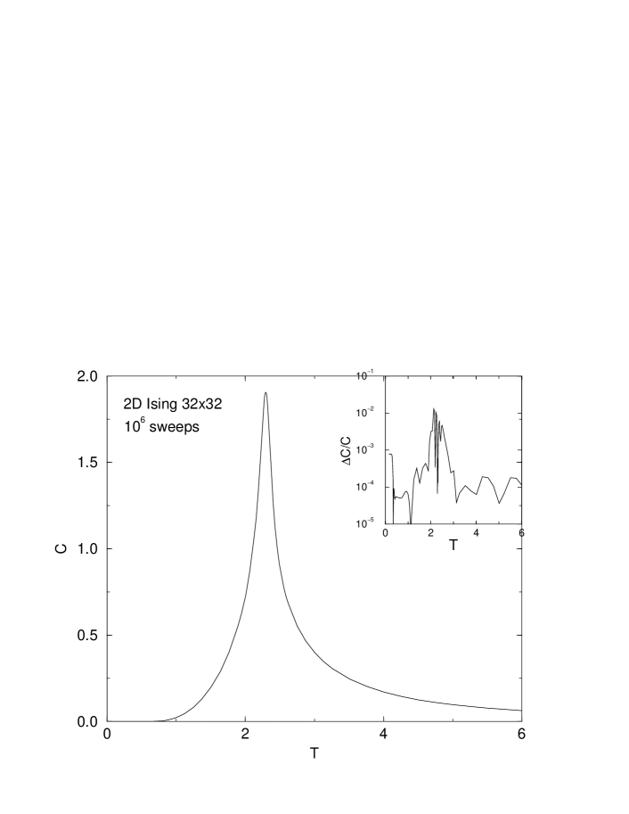
Figure 1: Specific heat for the two-dimensional Ising model computed by binary tree summation method. The insert gives the relative error with respect to exact result. The system size is $32\times 32$ with $10^{6}$ Monte Carlo sweeps.

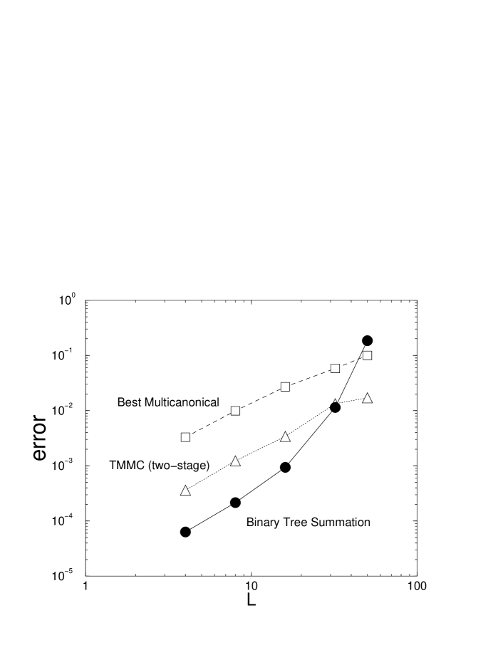
Figure 2: Average relative errors in $c_{b}$ after $10^{6}$ sweeps for the two-dimensional Ising model computed by binary tree summation method (circles), and errors in density of state $n(E)$ from multicanonical method (squares) and a two-stage transition matrix Monte Carlo method (triangles). The data are from ref. [18] and [9].

In Fig. 1, we present a plot of specific heat of the Ising model on a $32\times 32$ lattice. Errors in comparison with exact results [21] are indicated in the insert. For this lattice size, the errors are quite small for all values of $T$. In Fig. 2, we plot the average relative errors in $c_{b}$, defined by

$$\epsilon={1\over M}\sum_{b=0}^{M}\left|{c_{b}\over c_{b}^{\rm{exact}}}-1\right|.$$ (12)

The quantity $c_{b}$ plays the role of density of states as considered in refs. [22] and [23]. For the binary tree summation data, we have rescaled the error by a factor $\sqrt{t_{\rm cpu}/1.9}$ so that the comparison of errors is on an equal footing of given amount of CPU time. As we can see from the plot, the errors for small lattices are much smaller than that of both the multi-canonical simulation and transition matrix Monte Carlo method [9]. However, as the system size becomes larger than $32\times 32$, the error becomes comparable and less favorable to the other methods.

The decreased performance of binary tree summation method for large systems is partly due to the $O(N^{2})$ nature of the algorithm, and perhaps more importantly, it is not an importance sampling method. The fluctuation of the total weights $W_{b}$ in binary tree summation method is much smaller comparing to the $N$-fold way. Nevertheless, the weights introduce extra errors and become important for large systems. The $q=1$ percolation problem do not have such problem as in that case the total weight for each $b$ is a constant. A “fudge factor” may be introduced in the probability of choosing a type-1 bond with the aim to reduce the total weight fluctuation. We are still investigating on such possibilities.

4 Conclusion

We first compared the Sweeny and Gliozzi rates for the simulation of Potts models. The Sweeny and Gliozzi rates give the same dynamics and also do not completely eliminate critical slowing down. We then introduced Newman and Ziff method for simulating percolation problem. Our central goal is to simulate Potts models in the Fortuin-Kasteleyn representation in the spirit of Newman and Ziff. Binary tree summation method is our best attempt in this direction. Although the samples are generated without correlation between sweeps, we lost the property of importance sampling. In this sense, we have not completely solved the problem, thus the methods are not efficient for large systems. We hope the present work will stimulate research for algorithms that have zero correlation, yet realize importance sampling.

References

- [1] F. Y. Wu, Rev. Mod. Phys. 54, 235 (1982).
- [2] M. Sweeny, Phys. Rev. B 27, 4445 (1983).
- [3] P. W. Kasteleyn and C. M. Fortuin, J. Phys. Soc. Jpn Suppl. 26, 11 (1969); C. M. Fortuin and P. W. Kasteleyn, Physica 57, 536 (1972).
- [4] C.-K. Hu, Phys. Rev. B 29, 5103, 5109 (1984).
- [5] F. Gliozzi, cond-mat/0201285.
- [6] J.-S. Wang, O. Kozan, and R. H. Swendsen, in preparation.
- [7] R. H. Swendsen and J.-S. Wang, Phys. Rev. Lett. 58, 86 (1987).
- [8] U. Wolff, Phys. Rev. Lett. 62, 361 (1989); Nucl. Phys. B322, 759 (1989).
- [9] J.-S. Wang and R. H. Swendsen, J. Stat. Phys. 106, 245 (2002).
- [10] A. M. Ferrenberg, and R. H. Swendsen, Phys. Rev. Lett. 61, 2635 (1988); Phys. Rev. Lett. 63, 1195 and 1658 (1989).
- [11] B. A. Berg and T. Neuhaus, Phys. Rev. Lett. 68, 9 (1992).
- [12] P. M. C. de Oliveira, T. J. P. Penna, H. J. Herrmann, Braz. J. Phys. 26 (1996) 677; P. M. C. Oliveira, cond-mat/0204332.
- [13] F. Wang and D. P. Landau, Phys. Rev. Lett. 86, 2050 (2001).
- [14] M. Weigel, W. Janke, and C.-K. Hu, cond-mat/0107201.
- [15] B. A. Berg, Fields Inst. Commun. 26, 1 (2000).
- [16] C.-K. Hu, Phys. Rev. Lett. 69, 2739 (1992).
- [17] M. E. J. Newman and R. M. Ziff, Phys. Rev. Lett. 85, 4104 (2000); Phys. Rev. E 64, 016706 (2001).
- [18] J.-S. Wang, O. Kozan, and R. H. Swendsen, to appear in ‘Computer Simulation Studies in Condensed Matter Physics XV’, Eds. D. P. Landau, S. P. Lewis, and H. B. Schuettler (Springer Verlag, Berlin, 2002).
- [19] J. Hoshen and R. Kopelman, Phys. Rev. B 14, 3438 (1976).
- [20] J.-S. Wang, O. Kozan, and R. H. Swendsen, in preparation.
- [21] P. D. Beale, Phys. Rev. Lett. 76, 78 (1996).
- [22] C. Yamaguchi and N. Kawashima, cond-mat/0201527.
- [23] C. Yamaguchi, N. Kawashima, and Y. Okabe, cond-mat/0205578.