Decay Rate Distributions of Disordered Slabs and Application to Random Lasers

Abstract

We compute the distribution of the decay rates (also referred to as residues) of the eigenstates of a disordered slab from a numerical model. From the results of the numerical simulations, we are able to find simple analytical formulae that describe those results well. This is possible for samples both in the diffusive and in the localised regime. As example of a possible application, we investigate the lasing threshold of random lasers.

I Introduction

A very successful approach to describe disordered materials is supplied by random-matrix theory, see Refs. Beenakker, 1997; Guhr et al., 1998 for reviews. While one can put the beginning of random-matrix theory at Wigner’s surmise for describing the scattering spectra of heavy atomic nuclei,Wigner (1956) its theoretical foundations were laid only much later.Bohigas et al. (1984) It was very successfully applied to electronic transport in disordered wires and mesoscopic quantum dots, and recently these methods have been adopted to model (quantum) transport of optical radiation in media with spatially fluctuating dielectric constant.Beenakker (1998, 1999); Patra and Beenakker (1999a, b)

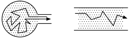
Figure 1: Two frequent geometries in the theory of disordered media are the chaotic cavity (left) and the disordered slab (right). The motion in the chaotic cavity is completely ergodic while in the disordered slab it is ergodic only in the transversal direction.

In the theoretical treatment of disordered materials, two particular geometries are of special importance, namely the disordered slab and the chaotic cavity (see Fig. 1). The principal difference between the geometries is easily explained: A chaotic cavity is an object in which the dynamics is chaotic due to the shape of the cavity or due to scatterers placed at random positions. The size of the opening is small compared to the total surface area of the cavity. Particles (electrons, photons) are then “trapped” inside the structure for a time that is long enough to ergodically explore the entire cavity. In a disordered slab, particles cannot be trapped that efficiently. They can no longer explore the entire volume ergodically but they still stay long enough to explore the entire cross-section of the sample, thus still making a random-matrix description possible. In order to call this geometry a “wire” or a “waveguide” its length should be much larger than its width. To be able to apply the theory only the much weaker criterion that the length is sufficiently larger than the mean-free path of the medium has to be fulfilled.

Two different aspects are of special important in the theory of disordered media, namely transport properties and resonances. The transport properties (moments of the eigenvalues of the transmission and reflection matrices) are known for the disordered slab in the limit that it is wide,Brouwer (1998) for the chaotic cavity with an opening that is so small that only one or two modes can propagate through it,Brouwer and Beenakker (1995, 1997) or a chaotic cavity with a wide opening.Beenakker (1999)

Less is known about the poles of such systems. (The eigenvalues of the Hamiltonian correspond to poles of the scattering matrix, and these show up as resonances in a scattering experiment. Hence the somewhat inconsistent nomenclature.) The beginning of random-matrix theory can be put at the moment when Wigner surmised the eigenvalue distribution for a closed chaotic cavity.Wigner (1956); Mehta (1990); Beenakker (1997) Here we are interested in open systems, where the eigenvalues acquire an imaginary part. (The imaginary part is referred to as residue.) It determines the decay rate of the (quasi-)eigenstate of the system. For chaotic cavities with broken time-reversal symmetry, the decay rate distribution is known analytically for an opening of arbitrary size.Fyodorov and Sommers (1997) The distribution for the more important case of preserved time-reversal symmetry is not known but can be approximated by a cavity with broken symmetry and an opening of half the real size.

Information on the residues of a disordered slab is very limited, and only the scaling behaviour of the large residue-tail in the localised regime was determined recently.Titov and Fyodorov (2000); Terraneo and Guarneri (2000a) This deficiency is felt especially strong in the random-laser community since the location of the residues gives the lasing threshold of an optical system, and most experimental setups resemble a disordered slab much more than they resemble a cavity. This paper fills this gap by presenting the results of numerical simulations. The quality of the numerical decay rate distributions is good enough that it allows us to arrive at analytical formulae for the distribution function, including its dependence on the parameters of the system. The idea to use high-quality simulations to arrive at formulae is not completely new as the distribution of the scattering strengths of chaotic cavities was found in the same way.Beenakker (1999)

This paper is organised as follows: First, we introduce the Anderson Hamiltonian used the describe the disordered slab. In Sec. III we show how the eigenvalues of that Hamiltonian can be computed in a efficient numerical way. Depending on the length of the slab, it can be in either the diffusive or in the localised regime. We will analyse the decay rate distributions for both regimes separately, first in Sec. V for the diffusive and then in Sec. VI for the localised regime. Until that point all results are completely general and can be applied to electronic and photonic systems. In Sec. VII we specialise on the lasing threshold in amplifying disordered media. We distinguish between the diffusive and the localised regimes (Secs. VII.1 and VII.2). We conclude in Sec. VIII.

II Anderson Hamiltonian for a disordered slab

We consider a two-dimensional slab of length $L$ and width $N$. The slab is described by an Anderson-type lattice Hamiltonian with spacing $1$. In the Anderson model, transport is modelled by nearest-neighbour hopping between lattice sites. Without loss of generality we can set the hopping rate to $1$. With a spatially varying potential $P(x,y)$ the Hamiltonian becomes

$$\mathcal{H}_{(x,y),(x,y)} =P(x,y) (y\neq 1,L)$$ (1a)

$$\mathcal{H}_{(x,y),(x,y)} =P(x,y)-i\kappa (y=1,L)$$ (1b)

$$\mathcal{H}_{(x,y),(x+1,y)} =1 (x<W)$$ (1c)

$$\mathcal{H}_{(x,y),(x-1,y)} =1 (x>1)$$ (1d)

$$\mathcal{H}_{(x,y),(x,y+1)} =1 (y<L)$$ (1e)

$$\mathcal{H}_{(x,y),(x,y-1)} =1 (y>1)$$ (1f)

All other elements are zero. $x$ runs from $1$ to $N$, and $y$ from $1$ to $L$.

The real part $E$ of the eigenvalues of $\mathcal{H}$ in the limit of large $N$ and $L$ is confined to the interval $[-4;4]$. (If the average of $P(x,y)$ is nonzero, the interval is simply shifted by that average. If $P(x,y)$ is fluctuating as a function of $x$ and $y$ — like it does for a disordered medium — the interval becomes a bit wider.) For electronic systems, $E$ gives the energy of the eigenstate, and Eq. (1) hence describes a slab with a conduction band of width $8$. For photonic systems, the real part of the eigenvalue gives the eigenfrequency. For both systems, the imaginary part $\gamma$ of the eigenvalue gives the decay rate of the eigenstate. (Actually not $\gamma$ but rather $\gamma/2$ is the decay rate but for the ease of notation we will continue to refer to $\gamma$ simply as the decay rate.)

$\kappa$ in Eq. (1b) quantifies the strength of the coupling between the slab and the outside.Fyodorov and Sommers (1997) Using the units introduced above, $\kappa$ has the value $\sin^{2}k$ where $k$ is the wavevector at the energy at which particles are injected respectively emitted. This quantity is proportional to the velocity of the particle perpendicular to the interface. In the centre of the band $\sin k=1$ whereas at the edges $\sin k=0$.

If $\kappa$ is chosen to be constant (i. e. not to depend on energy) ideal outcoupling can be described only for one specific value of the energy. We will do this since otherwise solving the Hamiltonian no longer is a standard eigenvalue problem, and set $\kappa\equiv 1$, hence modelling ideal coupling at the centre of the band. Working at the centre of the conduction bands offers the advantage that the width $N$ of the sample is identical to the number $N$ of propagating modes, and thus allows the describe the largest number of propagating modes for given size of the Hamiltonian (i. e. given numerical work). It is possible to include energy dependent coupling termsTerraneo and Guarneri (2000b) but it should be stressed that a constant $\kappa$ is more efficient and gives completely correct results as long as only eigenvalues near the respective energy are considered. We set $\kappa=1$, meaning ideal coupling at the centre of the conduction band.

It should be stressed that – even though we are modelling a two-dimensional system — the results are valid for three-dimensional systems as long as $L\gtrsim N$. A particle that is injected into the slab ergodically explores the entire cross-section of the sample before being emitted again, and hence loose its memory of which sites are “connected” by hopping terms. The sites can then be re-arranged, e. g. in a three-dimensional structure. Only for very short samples, $L\lesssim N$, this is not possible but for such samples already applying the Anderson model (i.e. only allowing nearest-neighbour hopping) is very questionable. The only “real” restriction that can limit the application of our results to certain photonic three-dimensional systems is that particles can leave the sample only at the front and at the back — and not through the “sides”.

In the formulation of Eq. (1) the matrix $\mathcal{H}$ has double indices but these are easily removed by considering $\mathcal{H}_{nn^{\prime}}$ with $n=x+(y-1)N$. (It would not make sense to set $n=y+(x-1)L$ since usually $L\gg N$, and we want to work with a band matrix that is as small as possible.) This results is a matrix of the form as depicted in Fig. 2. It is a banded $LN\times LN$ matrix with band width $2N+1$. Also within the band most elements are zero (since usually $N\gg 1$). The matrix is symmetric but non-Hermitian as there are complex numbers on the diagonal.

Figure 2: The Hamiltonian $\mathcal{H}$ has a band structure. The thin lines contain matrix elements that are mostly $1$, the diagonal is filled with complex numbers, and all other elements are zero. The entire matrix is symmetric but non-Hermitian (since there are complex elements on the diagonal).

The model (1) has been widely used since an efficient way to compute the transmission through such a slab is known.Baranger et al. (1991) The method of recursive Greens functions allows to compute the entire scattering matrix, hence all linear transport properties, in a time of order $\mathcal{O}(LN^{3})$ and with only minimal storage requirements $\mathcal{O}(N^{2})$. No explicit reference to the Hamiltonian $\mathcal{H}$ is made, so that eigenvalues cannot be computed by this method.

III Computing eigenvalues of symmetric complex non-Hermitian banded matrices

Since the Hamiltonian $\mathcal{H}$ from Eq. (1) is both banded and sparse one might be tempted to use an eigensolver for sparse matrices to compute the eigenvalues of Eq. (1). A sparse eigenvalue routine needs to be able to solve the equation

$$(\mathcal{H}-\mu\mathbbm{1})\vec{x}=\vec{y}$$ (2)

for the unknown vector $\vec{x}$ for arbitrary $\mu$ and $\vec{y}$. In particular, the eigensolver needs to set $\mu$ close to an eigenvalue of $\mathcal{H}$ so that the matrix $\mathcal{H}-\mu\mathbbm{1}$ is ill-conditioned. A numerical solution of Eq. (2) is then difficult and very expensive. Furthermore, only one eigenvalue is found at a time, and control of which eigenvalue the algorithm will converge to is difficult. (Algorithms for sparse matrices always use inverse iteration so that the corresponding eigenvector will be returned without additional effort but the eigenvector is of no use for us.) Using an algorithm for banded matrices is thus the better alternative.

There exist a number of algorithms for real symmetric or complex Hermitian band matrices. Both problems are characterised by real eigenvalues, so that they are conceptually identical. Only one algorithm for computing an eigenvalue (plus the corresponding eigenvector) of a general complex band matrix has been published.Schrauf (1991) It uses inverse iteration, so it is of limited use here.

We thus had to implement our own eigenvalue solver. The eigenrepresentation of $\mathcal{H}$ in terms of the diagonal matrix $\Lambda=\mathrm{diag}(\lambda_{1},\ldots,\lambda_{N})$ of the eigenvalues $\lambda_{i}$ of A and the matrix $U$ of eigenvectors is

$$\mathcal{H}=U\Lambda U^{-1}\;.$$ (3)

We now observe that for symmetric, that includes complex symmetric, $\mathcal{H}$ it is always possible to chose eigenvectors such that $UU^{T}=\mathbbm{1}$. If $U$ would be a real matrix, one would call $U$ orthogonal but since it is complex there is no special name for the property $UU^{T}=\mathbbm{1}$.

Algorithms for diagonalising a real symmetric matrix $A$ implicitly decompose $A$ as

$$A=QDQ^{T}\;,\qquad QQ^{T}=\mathbbm{1}$$ (4)

with the matrix $D$ of eigenvalues of $A$. It is therefore possible to adapt such an algorithm for our needs. Most algorithms for banded matrices first reduce $A$ to tridiagonal form $A^{\prime}$ by transformations of the form $A^{\prime}=Q^{\prime}AQ^{\prime T}$, and we will adopt this strategy. (A matrix is called tridiagonal if only the diagonal and its neighbouring elements are nonzero. If $A$ would be real, the transformation $A\to A^{\prime}$ would be called a similarity transformation.) For a band matrix this is possible in an efficient way since it is not necessary to compute (and thus store) the full matrices $Q^{\prime}$, and by annihilating the elements of the matrix $A$ in a clever order, the band structure is kept intact in all steps.Kaufman (1984, 2000)

The reduction of the complex matrix $\mathcal{H}$ to tridiagonal shape is done by straight-forward adaptation of this algorithm from real to complex numbers, where care needs to be taken that the dot product $\vec{x}\cdot\vec{y}=\sum_{i}x_{i}y_{i}$ is used and not the dot product $\vec{x}\cdot\vec{y}=\sum_{i}\overline{x}_{i}y_{i}$ normally used for complex vectors. (The overbar marks the complex conjugate.)

To compute the eigenvalues of the tridiagonal matrix for the real symmetric or complex Hermitian case, methods that isolate eigenvalues in disjunct intervals are used (“divide and conquer” and similar methodsGolub and van Loan (1989)). Such methods work for both of these cases as all eigenvalues are real and can thus be ordered. This no longer is possible here as the eigenvalues are complex. We therefore use the QR respectively QL method.Anderson et al. (1999)

For an $K\times K$ banded matrix with band width $W$ the time needed to compute the eigenvalues increases as $\mathcal{O}(K^{2}W)$ whereas the storage requirements increase as $\mathcal{O}(KW)$. In terms of the dimensions $L$ and $N$ of the disordered slab, this means that the time increases as $\mathcal{O}(L^{2}N^{3})$ and the storage space as $\mathcal{O}(LN^{2})$. For given computational resources, both scalings impose an upper limit on the system size that can feasible be treated. For typical values of the ratio $L$ and $N$, and for “realistic” computer equipment, the time limit is reached somewhat earlier than the memory limit.

With respect to a similar algorithm for full matrices one wins a factor $L$ (usually of order several hundred) for both time and memory by using the banded algorithm, thus allowing to treat system that could not be treated otherwise. Still, the work presented in this paper is a big numerical challenge. To arrive at the results, of the order of 100000 hours of cpu time on fast PC’s were needed.

IV Numerical simulations

Disorder is modelled by assigning random values to $P(x,y)$. It is assumed that those random numbers are uniformly distributed in the interval $[-w;w]$ so that $w$ measures the amount of disorder.

We only consider eigenvalues near the centre of the conduction band as the assumption of ideal coupling is only valid there. For numerical reasons it is essential that the centre of the conduction band is at $E=0$, i.e. one is not allowed to add an offset to $P(x,y)$.

Figure 3: Probability distribution of the decay rates for given system parameters as a function of the window size around the centre in which eigenvalues are included in computing the probability distribution. The different dots mark the distributions with $d=0.01$, $0.1$, $0.5$ and $1.0$.

We hence chose a window $[-d;d]$ and only include eigenvalues in the further analyses when their real part is inside that window. If the window is too large, systematic errors are introduced while too small a window leads to bad statistics. As can be seen from Fig. 3, for of $d=0.1$ the distribution function already agrees with the distribution function for $d=0.01$ but has much better statistics. $d=0.5$ and $d=1.0$ gives significant systematic deviations. For this reason, all results presented in this paper assume a window with $d=0.1$.

Figure 4: Mean free path $l$ as a function of disorder strength $w$ from a numerical simulation (crosses) and from Eq. (6).

The formulation of the model in Sec. II is in terms of generic units. Contact with a microscopic model or an experiment is best made in terms of the mean free path. It can be computed from the length-dependence of the transmission probability $T$ through the sample. In the diffusive regime, $l\lesssim L\ll Nl$, it is given by Beenakker (1997)

$$\frac{1}{T}=1+\frac{L}{l}\;.$$ (5)

The mean free path can be computed by fitting $T(L)$ to this functional form.

The transmission probability has been computed using the method of recursive Green’s functionsBaranger et al. (1991) for variable disorder strength $w$. As Fig. 4 shows, the numerically computed mean free path $l$ is for the range of $w$ in question in very good approximation given by

$$l=\frac{6}{w^{3/2}}\;.$$ (6)

(Computed for each value of $w$ from $50$ samples with $L=2,4,\ldots,98,100$ and $N=50$.) In the following, we will no longer make explicit reference to $w$ but rather give the more intuitive mean-free path $l$.

V Diffusive regime

For a sample length $L$ with $l\lesssim L\ll Nl$ the sample is said to be in the diffusive regime. It is immediately obvious that the diffusive regime can only be observed in sufficiently wide samples, $N\gg 1$.

For chaotic cavities with broken time-reversal symmetry an analytical result for the decay rate distribution has been given by Fyodorov and Sommers.Fyodorov and Sommers (1997) We start from their result and rescale it,

$$\mathcal{P}(y)=\frac{1}{y^{2}M!}\int_{0}^{My}x^{M}e^{-x}dx=\frac{1}{y^{2}}\left[1-e^{-My}\sum_{k=0}^{M}\frac{M^{k}}{k!}y^{k}\right]\;.$$ (7)

$\mathcal{P}(y)$ is normalised to one and in our scaling is for all $M>1$ peaked near a value of $y$ of order $1$. In the original formulation for a chaotic cavity, $M$ is the number of modes propagating through the opening of the cavity.

In the following we will argue that the decay rate distribution $P(g)$ can be written in the form (7) as

$$P(\gamma)=\frac{1}{\gamma_{0}}\mathcal{P}\bigl{(}\frac{\gamma}{\gamma_{0}}\bigr{)}$$ (8)

with some scaling factor $\gamma_{0}$ and some effective number of modes $M\neq N$. In Fig. 5 a comparison between the analytical suggestion and a simulation is given, and the agreement is striking. The horizontal axis has been plotted logarithmically since this results in both the differences between the $P(y)$ for different $N$ becoming easier to recognise and in giving a more prominent place to the small-$\gamma$ tail of $P(\gamma)$. In most applications, including the random laser discussed later in this paper, one is much more interested in small $\gamma$ than in large $\gamma$.

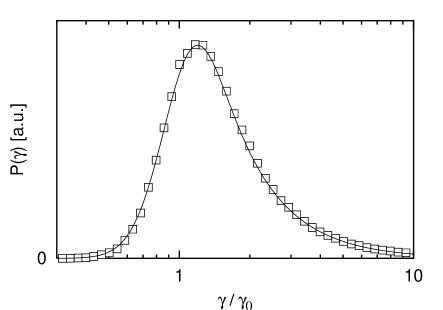
Figure 5: The numerically computed probability distribution $P(g)$ for $L=175$, $N=50$, $l=12.9$ and comparison with Eq. (7) with $M=16$.

The results of the simulations are fitted “by eye” against the functional form (7), resulting in one pair of values for $\gamma_{0}$ and $M$ for each set of parameters. Especially at very small $\gamma$, there are sometimes numerical errors that introduce artifacts into the numerical histogram so that using an automatic fitting algorithm is not feasible. (Usually we computed 500–1500 realisations for each parameter set.) From our simulations, we find that the scaling factor $\gamma_{0}$ only depends on the length $L$ of the sample and its mean free path $l$ but not on its width $N$, and seems to be given by

$$\gamma_{0}=\frac{2l}{L^{2}}\;.$$ (9)

As Fig. 6 shows, the agreement between the result of the numerical simulations and Eq. (9) is good, and all major deviations are for small $L$ where universal scaling is expected to be worse than for larger $L$. The model equations set the speed of propagation to $1$ but it is obvious that for some other choice for the propagation speed $c$ one has to change Eq. (9) to $\gamma_{0}=2cl/L^{2}$.

Figure 6: Scaling factor $\gamma_{0}$ as a function of $l$ and $L$ for $l=24$ and $N=10,20,50,100$ (open symbols) and $l=12.9$ and $N=50$ (solid circles). The line marks the prediction from Eq. 9.

Figure 7: Effective number $M$ of degrees of freedom as a function of the length $L$ of the sample for a sample with $N=30$, $N=50$ respectively $N=70$ propagating modes. The line marks the prediction from Eq. 10, the points are from numerical simulations. The size of the “errorbars” does not indicate some estimated error interval but simply marks the computed value $\pm 1$.

While the determination of $\gamma_{0}$ is very precise, there is a somewhat larger error involved in determining $M$ by fitting the analytical form to the results of numerical simulations. First, we only fitted against integer $M$, though in principle a generalisation of Eq. (7) to noninteger $M$ is possible, see Eq. (25). Secondly, if $M\gtrsim 25$, the difference between $P(y)$ for $M$ and for $M+1$ becomes too small to tell with certainty which of these two values describes the numerical result better. Thirdly and finally, even with 500-1500 samples for each set of parameter values, there are still some fluctuations in the numerically computed histogram for the decay rate distribution that in some cases make the decision on the right $M$ a bit difficult. Considering all of this, one should allow for an error of $1$ for $M$, and even of $2$ for $M\gtrsim 25$.

We have computed $M$ for a series of samples with increasing length for three different widths $N$. As Fig. 7 shows, the effective number $M$ of modes is well approximated by

$$M=\frac{N}{1+L/(6l)}\;.$$ (10)

The agreement between this suggested analytical form and the numerical simulation becomes better as the width $N$ of the sample is increased. From the simulations it is obvious that the functional form Eq. (10) is correct but there still is the (small) possibility that the factor $6$ might need to be replaced by a slightly smaller value. To answer this question with certainty, we would need to increase both $L$ and $N$ significantly. Unfortunately, such simulations are outside the present time and memory constraints.

Equations (7–10) give a good description of the decay rate distribution of a disordered slab in the diffusive regime, provided the slab is sufficiently wide. Since the transversal length scales are set by microscopic quantities (wave length of the light for optical systems, Fermi wave length for electronic systems), all macroscopic objects are “wide”.

Figure 8: Numerically computed distribution of the decay rate $\gamma$ for a sample in the localised regime ($L=71.55~{}l$, $N=15$) and comparison with the log-normal distribution (13).

Figure 9: Left: Transmission through the sample and position $\gamma_{0}$ of the maximum of the log-normal distribution as a function of the length of the sample (for $N=15$). There is a small but finite difference between the length scales for both quantities. Centre: Position $\gamma_{0}$ of the maximum of the log-normal distribution as a function of length for samples of different width $N$. Right: Prefactor in front of the exponential for $L=71.55~{}l$ for different $N$ [cf. Eqs. (14) and (15)]. The dashed line marks the curve $1.12/N^{2}$.

VI Localised regime

If the length $L$ of a disorder medium is increased, the phenomenon of localisation sets in once $L\gtrsim Nl$ (see Ref. Beenakker, 1997 for a review). In the localised regime the probability of transmission $T$ through the sample is reduced significantly and decays exponentially with the length $L$ of the sample. The length scale $\xi$ is called the localisation length, and can be computed from an ensemble of disordered slabs by computing the average of the logarithm of the transmission as a function of the length of the samples, hence

$$-L/\xi=\langle\ln T(L)\rangle\;.$$ (11)

One should note that this is not identical to fitting the transmission to $\langle T(L)\rangle\propto\exp(-L/\xi)$ since the large sample-to-sample fluctuations of $T(L)$ in the localised regime would give a value for $\xi$ that is off by a factor $4$. The localisation length can also be computed analytically from the mean-free path using the DPMK equation, with the resultEfetov and Larkin (1983a, b); Dorokhov (1982a, b, 1983a, 1983b)

$$\xi=\frac{N+1}{2}l\;,$$ (12)

and agrees well with our numerical results.

It is generally accepted that the distribution of the decay rates $\gamma$ (at least for small $\gamma$) in the localised regime is log-normal, i. e., $\ln\gamma$ is distributed according to a Gaussian distribution. Recent interest has rather been in the large-$\gamma$ tail which was shown to follow a power-law.Titov and Fyodorov (2000); Terraneo and Guarneri (2000a) In a log-normal distribution, most of the weight lies in the right tail, so those papers give a sufficient description for most of the eigenmodes. In the context of applications to random lasers we are, however, interested in the small decay rate tail, hence in the log-normal distribution.

To our knowledge, there is only a single paper by Titov and Fyodorov that gives explicit expressions for the parameters of that log-normal distribution.Titov and Fyodorov (2000) However, their analytical results are for a somewhat different system so it is difficult to tell whether they agree or disagree with our findings. We will return to this aspect at the end of this section. First, we want to present the results of our numerical simulations.

Using the log-normal ansatz, the distribution of the decay rates $\gamma$ is

$$P(\gamma)=b\exp\left(-\frac{(\log\gamma-\log\gamma_{0})^{2}}{\sigma^{2}}\right)\;.$$ (13)

The numerically computed histograms indeed follow this form, see Fig. 8, except for the large-$\gamma$ tail — as already mentioned above but this deviation is only seen in a log-log plot.

Fig. (9) shows in the left the numerically computed $\gamma_{0}$ as a function of $L$ for $N=15$. Also displayed is the localisation length $\xi$ computed numerically from the transmission, being in good agreement with the analytical prediction (12). The quality of the data is good enough to say with confidence that $\gamma_{0}$ decays exponentially with a length scale that is somewhat larger than $\xi$. Fig. (9) shows in the right the value of $\gamma_{0}$ also for two other values of $N$, and all three cases are well-described by introducing a numerical fitting factor $a$,

$$\gamma_{0}\propto\exp\left(-\frac{L}{a\xi}\right)\quad\mathrm{with}\quad a=1.12\;.$$ (14)

It is known that working at the centre of the conduction band when in the localised regime can introduce certain artefacts, especially in analytical approaches. Among other, the localisation length at the band centre can differ by approximately $10\,\%$ from the value outside the centre.Kappus and Wegner (1981) We have defined $\xi$ based on the transmission through the sample (at an energy corresponding to the band centre), and in transmission resonances at all energies can contribute. A numerical prefactor $a$ that differs by about $10\,\%$ from $1$ thus does not come as a complete surprise.

We still need to compute the proportionality factor appearing in Eq. (14). For this purpose we need to plot the ratio of the numerically computed $\gamma_{0}$ and the right-hand side of Eq. (14) for different values of $N$. We did this for $L=71.55~{}l$. Since this is a very expensive operation, we have computed a large number of samples only for $N=10,15,20$ so that their statistics is better than for the other values of $N$. An estimate of the error for these “better” data points has been included in the figure. This allows us to conclude that

$$\gamma_{0}=\frac{a}{N^{2}}\exp\left(-\frac{L}{a\xi}\right)\quad\mathrm{with}\quad a=1.12\;.$$ (15)

It should be noted that this equation contains two numerical coefficients, and there is no obvious reason why they should be identical. Still, we find that they both are approximately $a=1.12$.

Re-introducing “physical units” into Eq. (15) is a bit more difficult than it was for Eq. (9) where it was obvious that one simply has to multiply by the velocity of propagation $c$. Here one has to multiply by $c/\Delta$ where $\Delta$ is the perpendicular grid spacing. Due to the assumption of one propagating mode per (lateral) grid point made in Sec. II, $\Delta$ is not arbitrary but has a well-defined physical meaning. For the electronic case, $\Delta=\pi/k_{\mathrm{F}}$ with $k_{\mathrm{F}}$ the wave vector at the Fermi level, and for the photonic case $\Delta=2\lambda/\pi$ with $\lambda$ the wave length of the light (hence $c/\Delta=1/(4\nu)$).

Figure 10: Top: Comparison of the numerically computed $\sigma$ with the prediction from Eq. (16). Bottom: Comparison of the numerically computed prefactor [from dividing the numerical $\sigma$ by $(L/a\xi)^{2/3}$, cf. Eq. (16)] with the prediction $2/3$ for samples of $L=71.55~{}l$. For some values of $N$ a higher number of samples has been computed, so that the data quality is high enough to also compute an error estimate. This has been indicated in the figure.

Determining the width $\sigma$ of the distribution is more difficult since we can only use the left wing of the distribution — the right wing eventually turns into a power-law tail and thus no longer follows a log-normal distribution. Once again, we have accumulated more data for $N=10,15,20$ so that some indication of the error is possible for those three data points.

From our data, we propose the formula

$$\sigma=\frac{2}{3}\left(\frac{L}{a\xi}\right)^{2/3}\;,$$ (16)

where $a=1.12$ has the same value as in Eq. (15). As Fig. 10 shows, there clearly is no disagreement between the numerical data and Eq. (16). However, please remember that the $\frac{2}{3}$ should be thought of as a fitting factor that might not be exactly $2/3$ but perhaps rather $0.67$ or some other numerical factor.

Since the distribution is log-normal only for not too large $\gamma$ (remember the power-law tail for large $\gamma$) the normalisation is nontrivial [$P(\gamma)$ is not normalised to $1$ any longer!] and cannot be computed from $\gamma_{0}$ and $\sigma$. The constant $a$ in Eq. (13) is directly equal to the height of the peak of the numerically computed $P(\gamma)$. Since the total area underneath the numerically computed $P(y)$ (and hence its normalisation) is dominated by the large-$\gamma$ tail, $a$ has a relatively large error. Taking all the available data, the most likely value is

$$b=\frac{1}{N^{2}}\exp\left(\frac{L}{a\xi}\right)\;.$$ (17)

This value has been determined from a large number of simulations that for space reasons cannot be presented here. Unfortunately the quality of the data is not good enough to decide whether an additional prefactor $a=1.12$ should appear.

At the present it is not possible to tell whether our results agree with the ones put forward by Titov and Fyodorov.Titov and Fyodorov (2000) In particular, they arrive at

$$\gamma_{0}\propto\exp\left(-\frac{3L^{\prime}}{\xi}\right)\;,$$ (18)

whereas our finding (15) was $\gamma_{0}\propto\exp(-L/1.12\xi)$. There are two obvious differences between the model used by them and the model employed by us. First, for numerical reasons we work at the centre of the conduction band while they work near (but sufficiently far away from) the band edges. This might explain the factor $a=1.12$ that we have to introduce. Secondly and probably more importantly, they consider a system of length $L^{\prime}$ that is closed at one end whereas our systems have length $L$ and are open at both ends. It is obvious that a half-closed system of length $L^{\prime}$ corresponds to an open system of length $L>L^{\prime}$. Eq. (18) suggests that those two systems could be mapped into each other by setting $L\approx 3L^{\prime}$ but there is no further evidence to support this claim.

VII Lasing threshold of a random laser

A random laser is a laser where the necessary feedback is not due to mirrors at the ends of the laser but due to random scattering inside the medium.Wiersma et al. (1995); Wiersma and Lagendijk (1997); Beenakker (1999) We model the random laser as a disordered slab containing a dye that is able to amplify the radiation in a certain frequency interval with rate $1/\tau_{\mathrm{a}}$. The lasing threshold is the amplification rate at which the intensity of the emitted radiation diverges in a linear model. If saturation effects are included, the emitted intensity increases abruptly but finitely at crossing the lasing threshold.

The lasing threshold is given by the value of the smallest decay rate of all eigenmodes in the amplification window.Misirpashaev and Beenakker (1998) (Remember that $\gamma$ actually is twice the decay rate. On the other hand, also $1/\tau_{\mathrm{a}}$ enters the relevant formulae only with a prefactor $1/2$. $\gamma$ thus indeed gives the necessary amplification rate $1/\tau_{\mathrm{a}}$.) This is easily understood since this simply means that in the mode with the smallest decay rate the photons are created faster by amplification than they can leave the sample (=decay). It, however, also follows from a complete quantum mechanical analysis.Schomerus et al. (2000); Patra and Beenakker (1999b)

The distribution of the decay rate has been computed in this paper. A certain number $K$ of modes will be in the frequency window where amplification is possible. The lasing threshold is given by the smallest $\gamma$ of these $K$ modes. In a simple picture that is valid once $K\gg 1$ we can assume that the $K$ different $\gamma$’s are distributed independently according to $P(\gamma)$.Misirpashaev and Beenakker (1998) The distribution $\tilde{P}(\gamma)$ of the smallest mode and hence of the lasing threshold then becomes

$$\tilde{P}(\gamma)=KP(\gamma)\left[1-\int_{0}^{\gamma}P(\gamma^{\prime})d\gamma^{\prime}\right]^{K-1}\;.$$ (19)

For $K\neq 1$, the distribution $\tilde{P}(\gamma)$ of the lasing threshold is not longer identical to the distribution $P(\gamma)$ of the decay rate of each individual mode. In particular, not only the precise form of these two distribution will be different, but also the “typical” value of the lasing threshold can be different from the “typical” decay rate $\gamma_{0}$. Interestingly, for chaotic cavities in the diffusive regime it was found that the latter two quantities differ only insignificantlyFrahm et al. (2000); Schomerus et al. (2000) which might seem counter-intuitive. A slab geometry is more “complicated” in that the scaling $K\propto N$ “tries” to lower the lasing threshold with increasing $N$.

For $K\gg 1$ the distribution $\tilde{P}(\gamma)$ is sharply peaked around its maximum. The position $\gamma_{\mathrm{m}}$ of the maximum is given by the solution of the equation $d\tilde{P}(y_{\mathrm{m}})/d\gamma_{\mathrm{m}}=0$, hence

$$0=\frac{dP(\gamma_{\mathrm{m}})}{d\gamma_{\mathrm{m}}}\left[1-\int_{0}^{\gamma_{\mathrm{m}}}P(\gamma^{\prime})d\gamma^{\prime}\right]-(K-1)[P(\gamma_{\mathrm{m}})]^{2}\;.$$ (20)

While Eq. (19) is difficult to compute numerically due to the large exponent $K-1\gg 1$, in Eq. (20) this exponent no longer appears.

Eq. (20) depends on $P(\gamma)$ which in turn depends on the dimensions $L$ and $N$ of the system. In assuming that the number of propagating modes is equal to the width $N$ of the sample we already have made the assumption that the width (and hence also the length) is measured in units of $\lambda/2$. (The “$2$” accounts for polarisation.) The total number of modes in the sample thus is $LN$. We assume that a fraction $f$ of them is inside the amplification window of the dye, hence $K=fNL$. For simplicity we neglect complications as the shape of the mode profile. (It is easily incorporated into the numerics and we refrain from doing this just to prevent having to introduce even more parameters.) $f$ depends only on the chemical properties of the dye and not on the dimensions of the sample.

In the following we will show how to compute the most likely lasing threshold for samples in both the diffusive and in the localised regime.

VII.1 Lasing threshold in the diffusive regime

The change of the lasing threshold with increasing system size is influenced by a subtle interplay between $L$ and $N$ in determining the distribution $P(\gamma)$ and in determining the number $K=fNL$ of total modes.

If $K\gg 1$ the lasing mode has a decay rate in the low-$\gamma$ tail of $P(\gamma)$ (i.e. $\gamma<\gamma_{0}$ or $y<1$). The weight of this tail is

$$\int_{0}^{1}P(y)dy=\frac{M^{M-1}}{(M-1)!}e^{-M}\;,$$ (21)

and goes to zero as $M$ becomes larger. For $M\to\infty$ the tail disappears completely, as is already obvious from the asymptotic form of the distribution,

$$P_{M\to\infty}(y)=\left\{\begin{aligned} &0&(y<1)\\ &1/y^{2}&(y\geq 1)\end{aligned}\right.$$ (22)

With increasing $N$ and hence increasing $M$, the probability that a given mode has a small $y$ thus decreases rapidly. On the other hand, we are interested in the smallest decay rate out of $K$ modes, and $K$ increases linearly with $N$. This are two counter-acting effects, and it is not obvious which of these two is stronger.

The effect of an increase of the system size $L$, on the contrary, is obvious. First, the average decay rate $\gamma_{0}$ decreases according to Eq. (9). Secondly, $M$ decreases from Eq. (10), leading to even smaller values for $\gamma$ of the lasing mode.

There have been some analytical attempts to compute the lasing threshold for a chaotic cavity Frahm et al. (2000); Schomerus et al. (2000). For large $M$, the small-$y$ tail of Eq. (7) was approximated by

$$P(y)\approx\frac{1}{2M}\left[1+\mathrm{erf}\bigl{(}\sqrt{M/2}[y-1]\bigr{)}\right]\;.$$ (23)

This allows to arrive at scaling laws of the lasing threshold for variable $M$ at fixed $K$. Unfortunately, the difference between two counter-acting effects of an increase in $N$ are so small that Eq. (23) is a bit too crude for our needs.

We thus have to revert to a numerical procedure. Eq. (7) can be rewritten using the incomplete Gamma function

$$\Gamma(a,x)=\int_{x}^{\infty}t^{n-1}e^{-t}dt\;.$$ (24)

$\Gamma(a,0)$ reduces to the well-known Gamma function $\Gamma(a)$. For numerical reasons it is advisable to introduce the regularised Gamma function $Q(a,x)=\Gamma(a,x)/\Gamma(a)$. Fast numerical algorithms to compute $Q(a,x)$ exist. [Please note that in the literature the definitions of the regularised Gamma function sometimes disagree in that our $Q(a,x)$ is denoted as $1-Q(a,x)$.] Now we can express Eq. (7) and its derivative and integral as

$$P(y) =\frac{1}{y^{2}}\bigl{[}1-Q(M+1,My)\bigr{]}\;,$$ (25a)

$$\frac{dP(y)}{dy} =\frac{(My)^{M}}{y^{2}\Gamma(M)}e^{-My}-\frac{2}{y^{3}}\bigl{[}1-Q(M+1,My)\bigr{]}\;,$$ (25b)

$$\int_{0}^{y}P(y^{\prime})dy^{\prime} =\frac{1}{y}\bigl{[}Q(M+1,My)-1\bigr{]}+1-Q(M,My)\;,$$ (25c)

so that Eq. (20) can be evaluated efficiently.

VII.2 Lasing threshold in the localised regime

From Eq. (13) we directly arrive at

$$\frac{dP(\gamma)}{d\gamma} =-2b\frac{\ln\gamma-\ln\gamma_{0}}{\gamma\sigma^{2}}\exp\left[-\frac{(\ln\gamma-\ln\gamma 0)^{2}}{\sigma^{2}}\right]\;,$$ (26a)

$$\int_{0}^{\gamma}P(\gamma^{\prime})d\gamma^{\prime} =\frac{b\sqrt{\pi}\sigma\gamma_{0}}{2}e^{\sigma^{2}/4}\left[1+\mathrm{erf}\left(\frac{2\ln(\gamma/\gamma_{0})-\sigma^{2}}{2\sigma}\right)\right]\;.$$ (26b)

A further simplification is not possible, and we did not manage to find suitable approximations. Also for the localised regime we thus are restricted to a numerical evaluation.

VII.3 Numerical results

Figure 11: Most likely lasing threshold as a function of the length $L/l$ and the width $N$ of the sample. For $L/l\gtrsim N$ (the lower right part of the diagram) the sample is localised, for $L/l\lesssim N$ (the upper left part) the sample is diffusive. The diagonal line marks the division, and the results close to that line should thus be viewed with caution. The left diagram depicts the results for $f=0.1$, the central diagram for $f=0.001$. The right diagram again depicts the results for the localised regime with $f=0.1$ but the horizontal axis has been rescaled to $L/\xi$ instead of $L/l$. The numbers $x$ at the contour lines mean $10^{x}c/l$ in the diffusive regime, and $10^{x}c/\Delta$ in the localised regime.

The lasing threshold is computed numerically from Eq. (20), using the formulae from Secs. VII.1 and VII.2. Into the formulae presented there, we have to insert the correct dependence of the $\gamma_{0}$, $M$, $\sigma$, etc. on $L$ and $N$ that was presented earlier in this paper. Despite this complication the numerical calculation is straight forward as Eq. (20) possesses a single root only. Since this root has a change of sign, it is easily found numerically.

Fig. 11 shows the results for both the diffusive and the localised regimes, for both $f=0.1~{}l$ and $f=0.001~{}l$. (The mean-free path appears as a factor since the figure is in units $L/l$ and not $L$.) The formulae found in this paper are valid deep in the diffusive regime respectively deep in the localised regime. Near the cross over, hence near the line $L\approx Nl$, this condition is not fulfilled. The numerical values near the diagonal line in Fig. 11 should thus be viewed with caution.

As can be seen from the figure, in the diffusive regime with $N\gg L/l$ the lasing threshold becomes almost independent of the width $N$ of the sample (for sufficiently large $N$), and the most likely value of the lasing threshold is about

$$\gamma_{\mathrm{m}}\approx\frac{2cl}{L^{2}}\;,$$ (27)

hence the value given by Eq. (9). This means that even though $K\gg 1$, $P(y)$ for $y<1$ is already so small that it dominates over the large value of $K$. Differences between this simple approximation and the precise numerical result appear for finite $N$, with the size of this difference depending on $f$. However, for designing experiments it is obvious from the results presented here that the only feasible way to lower the lasing threshold of a random laser in the diffusive regime is increasing its length, not modifying its width.

As Fig. 11 shows, also in the localised regime there is only a small dependence on $f$. This means that in a log-normal distribution the weight of the left tail is so small that unless $K$ is exponentially large $\gamma_{\mathrm{m}}$ cannot become much smaller than the position $\gamma_{0}$ of the peak of the distribution. The difference to the diffusive regime is that the lasing threshold can be lowered efficiently not only by increasing the length but also decreasing the width $N$ and hence driving the system farther into localisation.

It is no surprise that samples in the localised regime generally have a lower lasing threshold than samples in the diffusive regime. We have shown that also the diffusive samples can have an “acceptably small” lasing threshold as it is trivial to make them very long (since there is no need to care much about their width). For both the diffusive and the localised regime, the typical decay rates of a single mode are comparable to the lasing threshold.

VIII Conclusions

We have numerically computed the distributions of the residues (or decay rates) of a disordered slab. The slab has length $L$, mean free path $l$, width respectively cross-sectional area $N$ ($N$ is given as number of propagating channels) and velocity of propagation $c$. We were able to “guess” simple analytical formulae that are able to describe the numerical results well.

For a sample in the diffusive regime ($L\lesssim Nl$) we found in Eqs. (7–10)

$$P(\gamma) =\frac{L^{2}}{2lc}\mathcal{\mathcal{P}}\bigl{(}\frac{\gamma L^{2}}{2lc}\bigr{)}\;,$$ (28a)

$$\mathcal{P}(y) =\frac{1}{y^{2}}\Bigl{[}1-\frac{\Gamma(1+\frac{N}{1+L/6l},\frac{Ny}{1+L/6l})}{\Gamma(1+\frac{N}{1+L/6l})}\Bigr{]}\;,$$ (28b)

where $\Gamma(a,x)$ is the incomplete Gamma function. The agreement between the numerical results and the proposed formulae is good, and there is the possibility that Eq. (28) might become exact in the limit $L/l\gg N\gg 1$. However, there is only numerical and no analytical evidence to back this claim.

For a sample in the localised regime ($L\gtrsim Nl$) with localisation length $\xi=(N+1)l/2$ we found in Sec. VI

$$P(\gamma)=\frac{1}{N^{2}}\exp\left(\frac{L}{a\xi}-\frac{(\log\gamma-\log\gamma_{0})^{2}}{\sigma^{2}}\right)\;,\quad a=1.12\;,$$

$$\gamma_{0}=\frac{a}{N^{2}}\exp\left(-\frac{L}{a\xi}\right)\;,\quad\sigma=\frac{2}{3}\left(\frac{L}{a\xi}\right)^{2/3}\;.$$ (29)

The quality of the simulations results in the localised regime is somewhat less than in the diffusive regime. For this reason, Eq. (29) should be understood as an approximate fit only, and it very probably differs from the exact relation, especially outside the band centre.

These results can be applied to both electronic and photonic systems. For photonic systems we have shown that under realistic assumptions the lasing threshold of a random laser is close to $\gamma_{0}$ both in the diffusive and in the localised regime. Eqs. (28) and (29) thus not only give the distribution of the decay rate of each individual mode but also a good estimate of the lasing threshold, i. e. the smallest decay rate of a large number of modes.