Randomly evolving trees I

Abstract

The random process of the tree evolution with continuous time parameter has been investigated. By introducing the notions of living and dead nodes a new model of random tree evolution has been constructed. It is assumed that at $t=0$ the tree is consisting of a single living node (root) from which the evolution may begin. This initial state is denoted by ${\mathcal{S}}_{0}$. At a certain time instant $\tau\geq 0$ the root produces $\nu\geq 0$ living nodes connected by lines to the root which becomes dead at the moment of the offspring production. $\tau$ and $\nu$ are random variables with known distribution functions. In the evolution process each of the new living nodes independently of the others evolves further like a root. The state $\mathcal{S}_{t}$ of the tree at time instant $t>0$ is defined by the actual numbers of living and dead nodes. It has been shown that the generating function of the probability to find a tree in a given state ${\mathcal{S}}_{t}$ at $t\geq 0$, assuming that at $t=0$ it was in the state ${\mathcal{S}}_{0}$, satisfies a non-linear integral equation. Analyzing the time dependence of the expectation value of the number of living nodes it has been recognized that three completely different types of evolution exist depending on the average number $q_{1}$ of nodes produced by one living node. If $q_{1}<1$, then the evolution is subcritical, if $q_{1}=1$, then it is critical, while in the case of $q_{1}>1$ is supercritical. It has been proved that in the case of subcritical evolution there is a time point at which the variance of the number of living nodes is maximal. By using the the generating function of the probability to find at time moment $t\geq 0$ a given number of nodes in the tree, the time dependence of the expectation value and the variance of tree size has been calculated. The joint distribution function of the numbers of living and dead nodes has been also derived, and the correlation between these node numbers has been determined as a function of time parameter. It has been proved that the correlation function converges to $\sqrt{3}/2$ independently of the distributions of $\nu$ and $\tau$ when $q_{1}\rightarrow 1$ and $t\rightarrow\infty$.

PACS: 02.50.-r, 02.50.Ey, 05.40.-a

1 Introduction

There is a growing interest in randomly evolving graphs since a large number of practically important problems can be analyzed in this way. In the last few years so many papers have been published in this field that any list of references would be far from complete by any standards. It is very fortunate that recently two outstanding review papers [1], [2] have been published and thus the author of the present paper does not feel obliged to cite the large amount of important references.

There are many different models for the random graphs and it would be difficult to give a precise classification of them. Probably the oldest model has been proposed by Erdős and Rényi [3], [4], [5]. In this model the initial state of the graph consists of fixed number $n$ of nodes that will be randomly connected during the evolution. The time is discrete and counted by the number of successively appearing lines. At time $t=1$ one of the ${n\choose 2}$ possible lines defined by the nodes is chosen out assuming that each of these lines has the same probability to be chosen. At time $t=2$ the second line is chosen out from the ${n\choose 2}-1$ possible lines all these being equiprobable. Continuing this process at time $t=N$ a random graph is formed which is consisting of $n$ fixed nodes and $N$ lines selected randomly. If $n$ is a large positive integer converging to infinity and $N$ is increasing from $1$ to ${n\choose 2}$ then the evolution of the graph passes through several (say five) clearly distinguishable phases.

One has to mention that random networks with fixed number of nodes usually show the so-called small-world effect, i.e. the average shortest path is small. This type of graphs can be created by randomly rewriting some of the lines of a regular ring graph. Watts and Strogatz [6] noticed many interesting properties of these graphs called small-world networks and a large number of papers [7], [8] was published recently on this subject.

There is another - more realistic - model [9] for the random evolution of graphs. In this model the number of nodes is not fixed, but to the contrary of the Erdős and Rényi model it is increasing in each discrete, equidistant time moment by addition of a new node connected randomly to one or several of the nodes already existing in the graph. The probability of a given connection between the new and one of the old nodes may depend on the number of links due to the node existing already. Many variants [10], [11] of this scale-free model have been recently investigated by using different inventive approximations. The one of the most intensively studied problem is the chracter of the degree distribution of nodes in graphs evolving randomly with various preferential linking. The number of exactly solvable (or solved) problems, however, is not very much, therefore, it seems to be worthwhile to study models which can be treated exactly.

It is known for long time that the random evolution of a tree  corresponds to a Galton-Watson process [12] which describes the formation of a population which starts at $t=0$ with one individual and in which at discrete time moments $t=1,2,\ldots$ each individual independently of the others produces a random number of offspring with the same distribution. There are many interesting papers [13] on this subject but it is hardly to find articles about the random processes of tree evolution with continuous time parameter. The purpose of is this paper is the study of these special random trees with the hope that it brings about new insight into the nature of branching processes.

This paper is organized as follows. In Section 2 the exact description of the random process is given, while in Section 3 the derivations of the basic equations for the generating functions can be found. The properties of average characteristics (expectation values, variances and correlation functions) are discussed in Section 4, and, finally, the conclusions are summarized in Section 5.

2 Description of the random process

We will study the random evolution of such trees which are consisting of living and dead nodes as well as lines connecting the nodes. The living node is unstable, and after a certain time $\tau$ may become dead. The lifetime $\tau$ is random variable, and denote by ${\mathcal{P}}\{\tau\in(t,t+dt)\}=dT(t)$ the probability of finding $\tau$ in the time interval $(t,t+dt)$. The dead node is inactive, cannot change its state, and is unable to interact with the other nodes.

The evolution process can be described as follows. Let us suppose that at time instance $t=0$ the tree consists of a single living node called root and denote by ${\mathcal{S}}_{0}$ this state of the tree. At the end of its life the root creates $\nu=0,1,2,\ldots$ new living nodes and after that it becomes immediately dead. The number of the offspring $\nu$ is random variable, and the probabilities ${\mathcal{P}}\{\nu=k\}=f_{k},\;\;k=0,1,2,\ldots$ are supposed to be known. The new living nodes are promptly connected to the dead one and independently of the others each of them can evolve further like a root. It means that the tree from its initial state ${\mathcal{S}}_{0}$ may evolve further by two mutually exclusive ways:

• the root does not die, and thus the tree remains in its initial state during the whole time interval $(0,t)$, or

• the root does die in an infinitesimally small subinterval $\;(t^{\prime},t^{\prime}+dt^{\prime})\in(0,t)\;$ and produces $j\geq 0$ new living nodes. Each of these nodes will evolve further in the remained time interval $(t^{\prime},t)$ independently of the others like the root.

Figure 1: First step of the tree evolution. The new state arises from the initial state which consists of a single root. Four of the possible new states are illustrated in Fig. The living nodes are denoted by white and the dead ones by black circles. $f_{0},f_{1},f_{2},f_{3},\ldots$ are the probabilities of producing $0,1,2,3,\ldots$ nodes by the dying root.

Fig. 1 shows the initial state of a tree consisting of a single root and illustrates four of the possible states which may be produced by the dying root. The probabilities of producing $0,1,2,3,\ldots$ living nodes are denoted by $f_{0},f_{1},f_{2},f_{3},\ldots$.

Figure 2: One of the realizations of a random tree at the time moment $t>0$. The nodes denoted by white circle are capable for the further evolution, while those denoted by black could not further evolve. The horizontal dashed lines indicate the time instances at which nodes were produced.

Fig. 2 illustrates one of the realizations of a random tree at the moment $t>0)$. One can see in Fig. 2 three white circles denoting the living nodes which are capable for the further evolution and a large number of the black circles denoting the dead nodes which are unable to produce new living nodes. It is to mention that each of the offspring is connected by a line to the dead precursor. If a dead node has $k$ outgoing lines then it will be called node of $k$th out-degree. It is obvious that a living tree must have living nodes, while a dead tree consists of dead nodes only.

In order to simplify our consideration we will assume that the distribution function of the lifetime $\tau$ of living nodes is exponential, i.e.

$$dT(t)=e^{-Qt}\;Q\;dt,$$ (1)

where $1/Q=t_{0}$ is the expectation value of the lifetime. In this case the evolution becomes a Markov process. It is assumed that the probabilities

$${\mathcal{P}}\{\nu=k\}=f_{k},\;\;\;\;\;\;k=0,1,2,\ldots$$ (2)

are the same for all living nodes. By introducing the generating function

$$q(z)=\sum_{k=0}^{\infty}f_{k}\;z^{k}$$ (3)

we can define the factorial moments of $\nu$ in the following way:

$$q_{r}=\left[\frac{d^{r}q(z)}{dz^{r}}\right]_{z=1}\;\;\;\;\;\;r=1,2,\ldots\;\;.$$

For the expectation value and the variance of $\nu$ we have

$${\bf E}\{\nu\}=q_{1}\;\;\;\;\;\;\mbox{and}\;\;\;\;\;\;{\bf D}^{2}\{\nu\}=q_{2}+q_{1}-q_{1}^{2}.$$ (4)

For the sake of later use we cite the relation

$${\bf E}\{(\nu-1)^{2}\}={\bf D}^{2}\{\nu\}+(1-q_{1})^{2}.$$ (5)

In order to characterize the random process of tree evolution we introduce the random functions $\mu_{\ell}(t)$ and $\mu_{d}(t)$ which are the actual numbers of the living and dead nodes, respectively, at time instant $t\geq 0$. It seems to be worthwhile to define the random function $\mu(t)=\mu_{\ell}(t)+\mu_{d}(t)$ which gives the total number of nodes, i.e. the actual value of the tree size at $t\geq 0$. Finally, let us denote by $\mu_{e}(t)$ the number of lines in a random tree at time instant $t\geq 0$. It is obvious that the equality $\mu_{e}(t)=\mu(t)-1$ is true with probability $1$ for all $t\geq 0$.

In the next Section we shall derive the basic equations for the generating functions of probabilities of the following random events: $\{\mu_{\ell}(t)=n_{\ell}\},\;\;\{\mu_{d}(t)=n_{d}\},\;\;\{\mu_{\ell}(t)=n_{\ell},\;\mu_{d}(t)=n_{d}\}$ and $\{\mu(t)=n\}$, provided that at $t=0$ the tree was in the state ${\mathcal{S}}_{0}$.

3 Derivation of the basic equations

3.1 Generating function equations

3.1.1 Probability distribution of the number of living nodes

The living nodes capable to produce new nodes at the end of their life are responsible for the evolution of the tree. It seems to be interesting to have an insight into the random process of the formation of living nodes. Let us denote by

$${\mathcal{P}}\{\mu_{\ell}(t)=n|{\mathcal{S}}_{0}\}=p^{(\ell)}(t,n)$$ (6)

the probability that the number of living nodes $\mu_{\ell}(t)$ is equal to $n$ at the time instant $t\geq 0$ provided that at $t=0$ the tree was in the state ${\mathcal{S}}_{0}$. By exploiting the rules of the random evolution described in Section 2 it can be easily shown that

$$p^{(\ell)}(t,n)=e^{-Qt}\;\delta_{n,1}+$$

$$Q\;\int_{0}^{t}e^{-Q(t-t^{\prime})}\left[f_{0}\;\delta_{n,0}+\sum_{k=1}^{\infty}f_{k}\;\sum_{n_{1}+\cdots+n_{k}=n}\;\prod_{j=1}^{k}\;p^{(\ell)}(t^{\prime},n_{j})\right]\;dt^{\prime},$$

and by using the probability generating function

$$g^{(\ell)}(t,z)=\sum_{n=0}^{\infty}p^{(\ell)}(t,n)\;z^{n},$$

we can prove that $g^{(\ell)}(t,z)$ satisfies the integral equation

$$g^{(\ell)}(t,z)=e^{-Qt}\;z+Q\;\int_{0}^{t}e^{-Q(t-t^{\prime})}\;q\left[g^{(\ell)}(t^{\prime},z)\right]\;dt^{\prime}.$$ (7)

It is an elementary task to prove that the integral equation (7) is equivalent to the differential equation

$$\frac{\partial g^{(\ell)}(t,z)}{\partial t}=-Q\;g^{(\ell)}(t,z)+Q\;q\left[g^{(\ell)}(t,z)\right],$$ (8)

with the initial condition

$$\lim_{t\downarrow 0}g^{(\ell)}(t,z)=z.$$

From the equation (7) or (8) the time dependence of the expectation value and the variance of the random function $\mu_{\ell}(t)$ can be easily calculated.

3.1.2 Probability distribution of the number of dead nodes

A living node producing offspring becomes dead, and we are interested in the probability that the number of dead nodes $\mu_{d}(t)$ is equal to $n$ at time instant $t\geq 0$ provided that at $t=0$ the tree was in the state ${\mathcal{S}}_{0}$. By introducing the notation

$${\mathcal{P}}\{\mu_{d}(t)=n|{\mathcal{S}}_{0}\}=p^{(d)}(t,n),$$ (9)

we can easily derive the following equation:

$$p^{(d)}(t,n)=e^{-Qt}\;\delta_{n,0}+$$

$$Q\;\int_{0}^{t}e^{-Q(t-t^{\prime})}\left[f_{0}\;\delta_{n,1}+\sum_{k=1}^{\infty}f_{k}\;\sum_{n_{1}+\cdots+n_{k}=n-1}\;\prod_{j=1}^{k}\;p^{(d)}(t^{\prime},n_{j})\right]\;dt^{\prime},$$

and by using the probability generating function

$$g^{(d)}(t,z)=\sum_{n=0}^{\infty}p^{(d)}(t,n)\;z^{n},$$ (10)

we can prove that $g^{(d)}(t,z)$ satisfies the integral equation

$$g^{(d)}(t,z)=e^{-Qt}+z\;Q\;\int_{0}^{t}e^{-Q(t-t^{\prime})}\;q\left[g^{(d)}(t^{\prime},z)\right]\;dt^{\prime}.$$ (11)

It is obvious that the equation (11) is equivalent to the differential equation

$$\frac{\partial g^{(d)}(t,z)}{\partial t}=-Q\;g^{(d)}(t,z)+z\;Q\;q\left[g^{(d)}(t,z)\right],$$ (12)

with the initial condition

$$\lim_{t\downarrow 0}g^{(d)}(t,z)=1.$$

3.1.3 Probability distribution of the total number of nodes

Denote by $\mu(t)=\mu_{\ell}(t)+\mu_{d}(t)$ the sum of the numbers of living and dead nodes at $t\geq 0$. Let us determine the probability of the random event $\{\mu(t)=n\}$ provided that at $t=0$ the tree was in the state ${\mathcal{S}}_{0}$. Introducing the notation

$${\mathcal{P}}\{\mu(t)=n|{\mathcal{S}}_{0}\}=p(t,n)$$ (13)

and defining the generating function

$$g(t,z)=\sum_{n=0}^{\infty}p(t,n)\;z^{n},$$ (14)

it can be easily shown that $g(t,z)$ satisfies the integral equation

$$g(t,z)=e^{-Qt}\;z+z\;Q\;\int_{0}^{t}e^{-Q(t-t^{\prime})}\;q\left[g(t^{\prime},z)\right]\;dt^{\prime}.$$ (15)

For the sake of completeness we are deriving from Eq. (15) the equivalent differential equation:

$$\frac{\partial g(t,z)}{\partial t}=-Q\;g(t,z)+Qz\;q\left[g(t,z)\right]$$

the initial condition of which is

$$\lim_{t\downarrow 0}g(t,z)=z.$$

3.1.4 Joint distribution of the numbers of living and dead nodes

We shall define now the probability

$${\mathcal{P}}\{\mu_{\ell}(t)=n_{\ell},\mu_{d}(t)=n_{d}|{\mathcal{S}}_{0}\}=p^{(\ell,d)}(t,n_{\ell},n_{d}),$$ (16)

where $n_{\ell}$ and $n_{d}$ are a non-negative integers. It is clear that $p^{(\ell,d)}(t,n_{\ell},n_{d})$ gives the probability that at the time instant $t>0$ the number of living and that of dead nodes in a randomly evolving tree are equal to $n_{\ell}$ and $n_{d}$, respectively, provided that at $t=0$ the tree was in the state ${\mathcal{S}}_{0}$. By exploiting the rules of the random evolution described in Section 2 it can be shown that

$$p^{(\ell,d)}(t,n_{\ell},n_{d})=e^{-Qt}\;\delta_{n_{\ell},1}\;\delta_{n_{d},0}+$$

$$Q\;\int_{0}^{t}e^{-Q(t-t^{\prime})}\left\{f_{0}\;\delta_{n_{\ell},0}\;\delta_{n_{d},1}+\sum_{k=1}^{\infty}f_{k}\;V^{(\ell,d)}(t^{\prime},n_{\ell},n_{d})\right\}\;dt,$$

where

$$V^{(\ell,d)}(t^{\prime},n_{\ell},n_{d})=\sum_{n_{\ell,1}+\cdots+n_{\ell,k}=n_{\ell}}\;\sum_{n_{d,1}+\cdots+n_{d,k}=n_{d}-1}\prod_{j=1}^{k}p^{(\ell,d)}(t^{\prime},n_{\ell,j},n_{d,j}).$$

Introducing the probability generating function

$$g^{(\ell,d)}(t,z_{\ell},z_{d})=\sum_{n_{\ell}=0}^{\infty}\;\sum_{n_{d}=0}^{\infty}p^{(\ell,d)}(t,n_{\ell},n_{d})\;z_{\ell}^{n_{\ell}}\;z_{d}^{n_{d}},$$ (17)

and taking into account the generating function defined by Eq. (3) we obtain the fundamental equation in the form:

$$g^{(\ell,d)}(t,z_{\ell},z_{d})=e^{-Qt}\;z_{\ell}+z_{d}\;Q\;\int_{0}^{t}e^{-Q(t-t^{\prime})}\;q\left[g^{(\ell,d)}(t^{\prime},z_{\ell},z_{d})\right]\;dt^{\prime},$$ (18)

which can be rewritten as a nonlinear differential equation

$$\frac{\partial g^{(\ell,d)}(t,z_{\ell},z_{d})}{\partial t}=-Q\;g^{(\ell,d)}(t,z_{\ell},z_{d})+z_{d}\;Q\;q\left[g^{(\ell,d)}(t,z_{\ell},z_{d})\right]$$ (19)

with initial condition

$$\lim_{t\downarrow 0}g^{(\ell,d)}(t,z_{\ell},z_{d})=z_{\ell}.$$

One has to note that the former equations (7) and (11) can be immediately derived from the integral equation (18).

3.1.5 Joint distribution of the numbers of living nodes and lines

As it has been already mentioned the living nodes are responsible for the evolution of the tree. It seems to be interesting to have a deeper insight into the interplay between the living nodes and lines during the tree evolution. For this purpose let us determine the probability that the number of living nodes $\mu_{\ell}(t)$ born in the time interval $(0,t)$ and the number of lines $\mu_{e}(t)$ produced in the same time interval are equal to $n_{\ell}$ and $n_{e}$, respectively, provided that at the time instant $t=0$ the tree was in the state ${\mathcal{S}}_{0}$. Introducing the notation

$${\mathcal{P}}\{\mu_{\ell}(t)=n_{\ell},\mu_{e}(t)=n_{e}|{\mathcal{S}}_{0}\}=p^{(\ell,e)}(t,n_{\ell},n_{e}),$$ (20)

we can easily derive the backward equation

$$p^{(\ell,e)}(t,n_{\ell},n_{e})=e^{-Qt}\;\delta_{n_{\ell},1}\;\delta_{n_{e},0}+$$

$$Q\;\int_{0}^{t}e^{-Q(t-t^{\prime})}\left[f_{0}\;\delta_{n_{\ell},0}\;\delta_{n_{e},0}+\sum_{k=1}^{\infty}f_{k}\;M_{k}(t^{\prime},n_{\ell},n_{e})\right]\;dt^{\prime},$$

where

$$M_{k}(t^{\prime},n_{\ell},n_{e})=\sum_{n_{\ell,1}+\cdots+n_{\ell,k}=n_{\ell}}\;\sum_{n_{e,1}+\cdots+n_{e,k}=n_{e}-k}\;\prod_{j=1}^{k}\;p^{(\ell,e)}(t^{\prime},n_{\ell,j},n_{e,j}).$$

The probability generating function

$$g^{(\ell,e)}(t,z_{\ell},z_{e})=\sum_{n_{\ell}=0}^{\infty}\;\sum_{n_{e}=0}^{\infty}p^{(\ell,e)}(t,n_{\ell},n_{e})\;z_{\ell}^{n_{\ell}}\;z_{e}^{n_{e}},$$ (21)

we obtain

$$g^{(\ell,e)}(t,z_{\ell},z_{e})=e^{-Qt}\;z_{\ell}+Q\;\int_{0}^{t}e^{-Q(t-t^{\prime})}\;q[z_{e}\;g^{(\ell,e)}(t^{\prime},z_{\ell},z_{e})]\;dt^{\prime}.$$ (22)

This is an important equation from which one can easily derive relations for the time dependence of factorial moments $\mu_{\ell}(t)$, and $\mu_{e}(t)$, and calculate the correlation function between them. The particular variant of the Eq. (22), namely:

$$g^{(\ell,e)}(t,z_{\ell}=z,z_{e}=1)=g^{(\ell)}(t,z)=e^{-Qt}\;z+Q\;\int_{0}^{t}e^{-Q(t-t^{\prime})}\;q\left[g^{(\ell)}(t^{\prime},z)\right]\;dt^{\prime}$$

is equivalent to Eq. (7), and by substitutions $z_{\ell}=1$ and $z_{e}=z$ one can obtain the integral equation

$$g^{(\ell,e)}(t,z_{\ell}=1,z_{e}=z)=g^{(e)}(t,z)=e^{-Qt}+Q\;\int_{0}^{t}e^{-Q(t-t^{\prime})}\;q\left[z\;g^{(e)}(t^{\prime},z)\right]\;dt^{\prime}$$

determining the generating function $g^{(e)}(t,z)={\bf E}\{z^{\mu_{e}}\}$.

The differential equation corresponding to (22) has the form:

$$\frac{\partial g^{(\ell,e)}(t,z_{\ell},z_{e})}{\partial t}=-Q\;g^{(\ell,e)}(t,z_{\ell},z_{e})+Q\;q\left[z_{e}\;g^{(\ell,e)}(t,z_{\ell},z_{e})\right],$$

with the initial condition

$$\lim_{t\downarrow 0}g^{(\ell,e)}(t,z_{\ell},z_{e})=z_{\ell}.$$

3.1.6 Remarks on generating function equations

In this Section we derived integral equations for the following generating functions:

$$g^{(\ell)}(t,z)={\bf E}\left\{z^{\mu_{\ell}(t)}\right\},\;\;\;\;\;\;g^{(d)}(t,z)={\bf E}\left\{z^{\mu_{d}(t)}\right\},\;\;\;\;\;\;g(t,z)={\bf E}\left\{z^{\mu(t)}\right\}$$

and

$$g^{(\ell,d)}(t,z_{\ell},z_{d})={\bf E}\left\{z_{\ell}^{\mu_{\ell}(t)}\;z_{d}^{\mu_{d}(t)}\right\},\;\;\;\;g^{(\ell,e)}(t,z_{\ell},z_{e})={\bf E}\left\{z_{\ell}^{\mu_{\ell}(t)}\;z_{e}^{\mu_{e}(t)}\right\}.$$

For the sake of simplicity let us denote by $\gamma(t,z)$  any of these generating functions. It can be shown [14] that the integral equation for $\gamma(t,z)$ has just one solution satisfying the conditions

$$|\gamma(t,z)|\leq 1,\;\;\;\;\forall\;\;|z|\leq 1\;\;\;\;\mbox{and}\;\;\;\;\lim_{z\uparrow 1}\;\;\gamma(t,z)=1.$$

It is important to mention that if $\lim_{z\uparrow 1}\;\gamma(t,z)<1$, then the number of the tree elements (nodes, lines) increases so rapidly that it reach $\infty$ in a finite time interval. In our further considerations, however, this explosion-like evolution will be excluded.

4 Average characteristics

4.1 Expectation values and variances

One of the simplest way to study the characteristic properties of tree evolution is to analyze the time dependence of factorial moments of the following random functions:

$$\mu_{\ell}(t),\;\;\;\;\mu_{d}(t),\;\;\;\;\mbox{and}\;\;\;\;\mu(t).$$

For the sake of simplicity let us denote by $\chi(t)$ any of these random functions and define the generating function

$$\gamma(t,z)={\bf E}\{z^{\chi(t)}\}.$$ (23)

According to the Abel’s theorem the $j$th factorial moment

$${\bf E}\{\chi(t)\;[\chi(t)-1]\;\cdots\;[\chi(t)-j+1]\}=m_{j}(t)=\left[\frac{\partial^{j}\gamma(t,z)}{\partial z^{j}}\right]_{z=1},$$ (24)

exists if and only if the series

$$\sum_{n=0}^{\infty}{\mathcal{P}}\{\chi(t)=n|{\mathcal{S}}_{0}\}\;n^{j},\;\;\;\;j=1,2,\ldots,$$

converges uniformly at any finite time instant $t>0$. It is well-known that the simple moments

$${\bf E}\{[\chi(t)]^{j}\}=m^{(j)}(t)$$

can be expressed by the factorial moments [15] by using the relation

$$m^{(j)}(t)=\sum_{i=0}^{j}{\mathcal{S}}(j,i)\;m_{i}(t),\;\;\;\;j=1,2,\ldots\;,$$ (25)

where ${\mathcal{S}}(j,i),\;\;i=0,1,\ldots,j$ are the Stirling numbers of the second kind.

In the further considerations we are going to deal with two important average characteristics of the random function $\chi(t)$, namely with the expectation value ${\bf E}\{\chi(t)\}=m_{1}(t)$ and the variance ${\bf D}^{2}\{\chi(t)\}=m_{2}(t)+m_{1}(t)\;[1-m_{1}(t)]$.

In order to calculate these average characteristics we do not have to know the distribution function of $\nu$, it is enough to know the values of the first and second factorial moments of $\nu$ only. In this case the distribution of $\nu$ we call arbitrary (a). However, if we are interested in solving the generating function equations, then we should have the exact form of the distribution of $\nu$. In the sequel, we will use two simple distributions, namely the Poisson (p)

$${\mathcal{P}}\{\nu=k\}=e^{-q1}\;\frac{q_{1}^{k}}{k!},$$

and the geometric (g)

$${\mathcal{P}}\{\nu=k\}=\frac{1}{1+q_{1}}\;\left(\frac{q_{1}}{1+q_{1}}\right)^{k}.$$

distributions. In the case of the Poisson distribution we have

$${\bf E}\{\nu\}=q_{1}\;\;\;\;\;\;\mbox{and}\;\;\;\;\;\;{\bf D}^{2}\{\nu\}=q_{1},$$

while in that of the geometric one

$${\bf E}\{\nu\}=q_{1}\;\;\;\;\;\;\mbox{and}\;\;\;\;\;\;{\bf D}^{2}\{\nu\}=q_{1}(1+q_{1}).$$

4.1.1 Living nodes

Let as investigate the expectation value and the variance of the number of living nodes at the time instant $t>0$. The equation for the expectation value ${\bf E}\{\mu_{\ell}(t)\}=m_{1}^{(\ell)}(t)$ can be immediately derived from the Eq. (8). We obtain

$$m_{1}^{(\ell)}(t)=e^{-Qt}+Q\;q_{1}\;\int_{0}^{t}e^{-Q(t-t^{\prime})}\;m_{1}^{(\ell)}(t^{\prime})\;dt^{\prime},$$

which is a typical renewal equation. After elementary calculations the solution is obtained in the form:

$$m_{1}^{(\ell)}(t)=e^{-(1-q_{1})Qt},$$ (26)

from which we see that the average number of the living nodes has the following asymptotic properties:

$$\lim_{t\rightarrow\infty}=\left\{\begin{array}[]{ll}0,&\mbox{if $q_{1}<1$,}\\ 1,&\mbox{if $q_{1}=1$,}\\ \infty,&\mbox{if $q_{1}>1$. }\end{array}\right.$$ (27)

The evolution of the tree will be called subcritical, if $q_{1}<1$, critical, if $q_{1}=1$, and supercritical, if $q_{1}>1$.

In order to calculate the variance ${\bf D}^{2}\{\mu_{\ell}(t)\}$ we need the second factorial moment $m_{2}^{(\ell)}(t)$ which can obtained by solving the integral equation

$$m_{2}^{(\ell)}(t)=Q\;\int_{0}^{t}e^{-Q(t-t^{\prime})}\left\{q_{1}\;m_{2}^{(\ell)}(t^{\prime})+q_{2}\;\left[m_{1}^{(\ell)}(t^{\prime})\right]^{2}\right\}\;dt^{\prime}.$$

It is easy to show that

$$m_{2}^{(\ell)}(t)=\left\{\begin{array}[]{ll}\frac{q_{2}}{1-q_{1}}\;[1-e^{-(1-q_{1})Qt}]\;e^{-(1-q_{1})t},&\mbox{if $q_{1}\not=1$,}\\ \mbox{ }&\mbox{ }\\ q_{2}\;Qt,&\mbox{if $q_{1}=1$,}\end{array}\right.$$ (28)

and by using the relation

$${\bf D}^{2}\{\mu_{\ell}(t)\}=m_{2}^{(\ell)}(t)+m_{1}^{(\ell)}(t)\;[1-m_{1}^{(\ell)}(t)]$$

we have

$${\bf D}^{2}\{\mu_{\ell}(t)\}=\left\{\begin{array}[]{ll}\frac{{\bf E}\{(\nu-1)^{2}\}}{1-q_{1}}\;[1-e^{-(1-q_{1})Qt}]\;e^{-(1-q_{1})Qt},&\mbox{if $q_{1}\not=1$,}\\ \mbox{ }&\mbox{ }\\ q_{2}\;Qt,&\mbox{if $q_{1}=1$,}\end{array}\right.$$ (29)

where ${\bf E}\{(\nu-1)^{2}\}=(1-q_{1})^{2}+{\bf D}^{2}\{\nu\}$. In the case of subcritical ($q_{1}<1$) evolution the variance has a maximum at

$$x_{max}=Q\;t_{max}=\frac{\log 2}{1-q_{1}},$$

which is independent of the form of the distribution of $\nu$.

Figure 3: The variance of the number of living nodes vs. time parameter $Qt$ in subcritical ($q_{1}=0.95$) evolution. The curves g, p, and a correspond to the geometric, Poisson, and the arbitrary distributions of $\nu$, respectively. In the case of the arbitrary distribution the value ${\bf D}^{2}\{\nu\}=0.9$ has been chosen.

The variance vs. $Qt$ is shown in Fig. 3. The curves g, p, and a correspond to the geometric, Poisson, and arbitrary distributions of $\nu$, respectively. In the case of the arbitrary distribution the value ${\bf D}^{2}\{\nu\}=0.9$ has been chosen. The sites of maxima of curves ${\bf g,p}$ and ${\bf a}$ are the same, but the heights of the maxima depend, however, on the character of the distribution of $\nu$.

The relative variance of the number of living nodes at the time instant $t$ can be written in the form:

$$\frac{{\bf D}^{2}\{\mu_{\ell}(t)\}}{\left[{\bf E}\{\mu_{\ell}(t)\}\right]^{2}}=\left\{\begin{array}[]{ll}\frac{{\bf E}\{(\nu-1)^{2}\}}{1-q_{1}}\;[e^{(1-q_{1})Qt}-1],&\mbox{if $q_{1}\not=1$,}\\ \mbox{ }&\mbox{ }\\ q_{2}\;Qt,&\mbox{if $q_{1}=1$,}\end{array}\right.$$ (30)

from which it is evident that the relative variance is increasing with $t$ to $\infty$ in the subcritical and critical evolutions ($q_{1}\leq 1$), and converging to the saturation value

$$\frac{{\bf E}\{(\nu-1)^{2}\}}{q_{1}-1},$$

if the evolution is supercritical ($q_{1}>1$). It is trivial but interesting to note that the standardized expectation value of $\mu_{\ell}(t)$ has the form:

$$\frac{{\bf E}\{\mu_{\ell}(t)\}}{{\bf D}\{\mu_{\ell}(t)\}}=\left\{\begin{array}[]{ll}\left(\frac{1-q_{1}}{{\bf E}\{(\nu-1)^{2}\}}\right)^{1/2}\;\left[e^{(1-q_{1})Qt}-1\right]^{-1/2},&\mbox{if $q_{1}\neq 1$,}\\ \mbox{ }&\mbox{ }\\ \frac{1}{\sqrt{q_{2}}}\;(Qt)^{-1/2},&\mbox{if $q_{1}=1$.}\end{array}\right.$$ (31)

If the evolution is critical, then the standardized expectation value of the number of living nodes converges to zero as $(Qt)^{-1/2}$ when $t\Rightarrow\infty$.

4.1.2 Dead nodes

It is obvious that the number of dead nodes $\mu_{d}(t)$ in an evolving tree is a non-decreasing random function of time. From Eq. (11) we obtain for the expectation value ${\bf E}\{\mu_{d}(t)\}=m_{1}^{(d)}(t)$ the following equation:

$$m_{1}^{(d)}(t)=1-e^{-Qt}+q_{1}\;Q\;\int_{0}^{t}e^{-Q(t-t^{\prime})}\;m_{1}^{(d)}(t^{\prime})\;dt^{\prime},$$ (32)

the solution of that can be written in the form:

$$m_{1}^{(d)}(t)=\left\{\begin{array}[]{ll}\frac{1}{1-q_{1}}\;\left[1-e^{-(1-q_{1})Qt}\right],&\mbox{if $q_{1}\neq 1$,}\\ \mbox{ }&\mbox{ }\\ Qt,&\mbox{if $q_{1}=1$.}\end{array}\right.$$ (33)

We see that the expectation value of dead nodes converges to $(1-q_{1})^{-1}$ in subcritical and becomes infinite in critical and supercritical evolution when $t\Rightarrow\infty$. It is remarkable that the increase of $m_{1}^{(d)}(t)$ with time $t$ is linear in critical state.

In order to calculate the variance ${\bf D}^{2}\{\mu_{d}(t)\}$ of the number of dead nodes at the time instant $t\geq 0$ we have to solve the integral equation

$$m_{2}^{(d)}(t)=q_{1}\;Q\;\int_{0}^{t}e^{-Q(t-t^{\prime})}\;m_{2}^{(d)}(t^{\prime})\;dt^{\prime}+$$

$$Q\;\int_{0}^{t}e^{-Q(t-t^{\prime})}\;\left\{2q_{1}\;m_{1}^{(d)}(t^{\prime})+q_{2}\;\left[m_{1}^{(d)}(t^{\prime})\right]^{2}\right\}\;dt^{\prime},$$ (34)

which can be derived from Eq. (11) by using the formula

$$m_{2}^{(d)}(t)=\left[\frac{\partial^{2}g^{(d)}(t,z)}{\partial z^{2}}\right]_{z=1}.$$ (35)

After elementary calculations we obtain the solution in the form:

$$m_{2}^{(d)}(t)=a_{1}^{(d)}\;[1-e^{-(1-q_{1})Qt}]+$$

$$a_{2}^{(d)}\;Qt\;e^{-(1-q_{1})Qt}+a_{3}^{(d)}\;e^{-(1-q_{1})Qt}\;[1-e^{-(1-q_{1})Qt}],\;\;\;\mbox{if}\;\;\;q_{1}\neq 1,$$ (36)

where

$$a_{1}^{(d)}=\frac{1}{(1-q_{1})^{2}}\left(2\;q_{1}+\frac{q_{2}}{1-q_{1}}\right),\;\;\;\;a_{2}^{(d)}=-\frac{2}{1-q_{1}}\left(q_{1}+\frac{q_{2}}{1-q_{1}}\right),$$

and

$$a_{3}^{(d)}=\frac{q_{2}}{(1-q_{1})^{3}}.$$

If $q_{1}=1$, then we have

$$m_{2}^{(d)}(t)=(Qt)^{2}+\frac{1}{3}\;q_{2}\;(Qt)^{3}.$$ (37)

By using the expression

$${\bf D}^{2}\{\mu_{d}(t)\}=m_{2}^{(d)}(t)+m_{1}^{(d)}(t)\;[1-m_{1}^{(d)}(t)]$$

if $q_{1}\neq 1$, then we find

$${\bf D}^{2}\{\mu_{d}(t)\}=v_{1}^{(d)}\;[1-e^{-(1-q_{1})Qt}]+$$

$$v_{2}^{(d)}\;Qt\;e^{-(1-q_{1})Qt}+v_{3}^{(d)}\;e^{-(1-q_{1})Qt}\;[1-e^{-(1-q_{1})Qt}],$$ (38)

where

$$v_{1}^{(d)}=\frac{{\bf D}^{2}\{\nu\}}{(1-q_{1})^{3}},\;\;\;\;v_{2}^{(d)}=-2\;\frac{{\bf D}^{2}\{\nu\}}{(1-q_{1})^{2}},\;\;\;\;v_{3}^{(d)}=\frac{{\bf E}\{(\nu-1)^{2}\}}{(1-q_{1})^{3}},$$

and if $q_{1}=1$, i.e. the evolution is critical, then

$${\bf D}^{2}\{\mu_{d}(t)\}=Qt+\frac{1}{3}\;q_{2}\;(Qt)^{3}.$$ (39)

One can see that the limit values of the variance of the number of dead nodes are given by the formula

$$\lim_{t\rightarrow\infty}{\bf D}^{2}\{\mu_{d}(t)\}=\left\{\begin{array}[]{ll}\frac{{\bf D}^{2}\{\nu\}}{(1-q_{1})^{3}},&\mbox{if $q_{1}<1$,}\\ \mbox{}&\mbox{}\\ \infty,&\mbox{if $q_{1}\geq 1$.}\end{array}\right.$$

4.1.3 Total number of nodes

For many purposes, it may be important to know how the expectation value and the variance of the random function

$$\mu(t)=\mu_{\ell}(t)+\mu_{d}(t)$$ (40)

depend on the time. By using Eq. (15) one can derive integral equations the factorial moments

$$m_{1}(t)={\bf E}\{\mu(t)\} = \left[\frac{\partial g(t,z)}{\partial z}\right]_{z=1},$$ (41)

$$m_{2}(t)={\bf E}\{\mu(t)[\mu(t)-1]\} = \left[\frac{\partial^{2}g(t,z)}{\partial z^{2}}\right]_{z=1}.$$ (42)

After a brief calculation we obtain that

$$m_{1}(t)=1+q_{1}\;Q\;\int_{0}^{t}e^{-Q(t-t^{\prime})}\;m_{1}(t^{\prime})\;dt^{\prime},$$ (43)

and

$$m_{2}(t)=q_{1}\;Q\;\int_{0}^{t}e^{-Q(t-t^{\prime})}\;m_{2}(t^{\prime})\;dt^{\prime}+$$

$$Q\;\int_{0}^{t}e^{-Q(t-t^{\prime})}\;\left\{2q_{1}\;m_{1}(t^{\prime})+q_{2}\;\left[m_{1}(t^{\prime})\right]^{2}\right\}\;dt^{\prime}.$$ (44)

The solution of Eq. (43) has the form:

$$m_{1}(t)=\left\{\begin{array}[]{ll}(1-q_{1})^{-1}\;\left[1-q_{1}\;e^{-(1-q_{1})Qt}\right],&\mbox{if $q_{1}\neq 1$,}\\ \mbox{ }&\mbox{ }\\ 1+Qt&\mbox{if $q_{1}=1$,}\end{array}\right.$$ (45)

and looking at Eqs. (26) and (33) we can see the trivial identity

$$m_{1}(t)=m_{1}^{(\ell)}(t)+m_{1}^{(d)}(t)$$

to be valid. For the purpose of the calculation of the variance

$${\bf D}^{2}\{\mu(t)\}=m_{2}(t)+m_{1}(t)[1-m_{1}(t)]$$

we have to obtain the solution of Eq. (44). By having this solution we can immediately write:

$${\bf D}^{2}\{\mu(t)\}=$$

$$\frac{{\bf D}^{2}\{\nu\}}{(1-q_{1})^{3}}\;\left[1-e^{-(1-q_{1})Qt}\right]-2q_{1}\;\frac{{\bf D}^{2}\{\nu\}}{(1-q_{1})^{2}}\;Qt\;e^{-(1-q_{1})Qt}+$$

$$q_{1}^{2}\;\frac{{\bf E}\{(\nu-1)^{2}\}}{(1-q_{1})^{3}}\;e^{-(1-q_{1})Qt}\;\left[1-e^{-(1-q_{1})Qt}\right],\;\;\;\mbox{if}\;\;\;q_{1}\neq 1,$$ (46)

and in the case of critical evolution, i.e. if $q_{1}=1$, than we have a simple formula:

$${\bf D}^{2}\{\mu(t)\}=(1+q_{2})\;Qt+q_{2}\;(Qt)^{2}+\frac{1}{3}\;q_{2}\;(Qt)^{3}.$$ (47)

The average tree size at a given time instant $t>0$ can be characterized by the expectation value of the total number of nodes $\mu(t)$, but it is to mention that the actual sizes of randomly evolving trees may fluctuate significantly around the expectation value ${\bf E}\{\mu(t)\}$. This fluctuation can be measured by the relative variance

$$\frac{{\bf D}^{2}\{\mu(t)\}}{\left[{\bf E}\{\mu(t)\}\right]^{2}}={\bf VR}\{\mu(t)\}$$

the time dependence of which shows interesting features. We see from Eq. (45)    that the average tree size converges to infinity with $\;t\Rightarrow\infty\;$, if $q_{1}\geq 1$, and to $(1-q_{1})^{-1}$, if $q_{1}<1$.

Figure 4: Fig. A shows the relative variance of the total number of nodes vs. time parameter $Qt$. In Fig. B it can be seen at $Qt=\infty$ the dependence of relative variances on parameter $q_{1}$. In both Figs. the curves g, p, and a correspond to the geometric, Poisson, and the arbitrary distributions of $\nu$, respectively. In the case of the arbitrary distribution ${\bf D}^{2}\{\nu\}=0.9$ has been chosen for the calculations.

On the contrary, the relative variance remains finite when $t\Rightarrow\infty$ in the case of $q_{1}\neq 1$, and if and only if the evolution is critical, i.e., if $q_{1}=1$, then can be observed the relative variance to become infinite when $t\Rightarrow\infty$.

In the part A of Fig. 4 three curves of the relative variance of $\mu(t)$ versus $Qt$ are plotted when $q_{1}=0.95$. In the part B the dependence of the relative variance at $Qt=\infty$ can be seen on the parameter $q_{1}$. In both parts of Fig. the curves g, p, and a correspond to the geometric, Poisson, and the arbitrary distributions of $\nu$, respectively. At $q_{1}=1$ one can observe singularity in the relative variance, and thus one has to conclude that the average tree size at large $Qt$ cannot characterize the random evolution in critical state.

4.2 Covariances and correlations

The study of how the random functions $\mu_{\ell}(t),\mu_{d}(t)$ and $\mu_{e}(t)$ are related involves the analysis of at least two correlation functions. In the following we will investigate correlations between the living and dead nodes, as well as the lines and living nodes.

4.2.1 Living and dead nodes

In Sub-subsection 3.1.4 we derived an integral equation [see Eq. (18)] for the generating function $g^{(\ell,d)}(t,z_{\ell},z_{d})$ of the joint distribution $p^{(\ell,d)}(t,n_{\ell},n_{d})$ of random functions $\mu_{\ell}(t)$ and $\mu_{d}(t)$. It is clear that $p^{(\ell,d)}(t,n_{\ell},n_{d})$ gives the probability that at time instant $t\geq 0$ the number of living and that of dead nodes in a randomly evolving tree are equal to $n_{\ell}$ and $n_{d}$, respectively, provided that at $t=0$ the tree was in the state ${\mathcal{S}}_{0}$.

Covariance function.    In order to calculate the covariance function

$${\bf Cov}\{\mu_{\ell}(t)\mu_{d}(t)\}={\bf E}\{\mu_{\ell}(t)\mu_{d}(t)\}-{\bf E}\{\mu_{\ell}(t)\}{\bf E}\{\mu_{d}(t)\}$$ (48)

we need the equation determining the moment

$${\bf E}\{\mu_{\ell}(t)\mu_{d}(t)\}=\left[\frac{\partial^{2}g^{(\ell,d)}(t,z_{\ell},z_{d})}{\partial z_{\ell}\partial z_{d}}\right]_{z_{\ell}=z_{d}=1}=m_{1,1}^{(\ell,d)}(t).$$ (49)

The equation can be written in the form:

$$m_{1,1}^{(\ell,d)}(t)=Q\;q_{1}\;\int_{0}^{t}e^{-Q(t-t^{\prime})}\;m_{1,1}^{(\ell,d)}(t^{\prime})\;dt^{\prime}+$$

$$Q\;\int_{0}^{t}e^{-Q(t-t^{\prime})}\left[q_{1}\;m_{1}^{(\ell)}(t^{\prime})+q_{2}\;m_{1}^{(\ell)}(t^{\prime})\;m_{1}^{(d)}(t^{\prime})\right]\;dt^{\prime}.$$ (50)

By using the Eqs. (26) and (33) for $m_{1}^{(\ell)}(t)$ and $m_{1}^{(d)}(t)$, respectively, and introducing the notation $\alpha=(1-q_{1})\;Q$, it can be proved that

$$m_{1,1}^{(\ell,d)}(t)=\frac{{\bf D}^{2}\{\nu\}}{1-q_{1}}\;Qt\;e^{-\alpha t}-q_{2}\;\frac{1}{(1-q_{1})^{2}}\;e^{-\alpha t}\;(1-e^{-\alpha t}),$$

is the unique solution of the integral equation (50) $\forall\;\;q_{1}\neq 1$. After a brief calculation we have

$${\bf Cov}\{\mu_{\ell}(t)\mu_{d}(t)\}=\frac{{\bf D}^{2}\{\nu\}}{1-q_{1}}\;Qt\;e^{-\alpha t}-\left[1+\frac{{\bf D}^{2}\{\nu\}}{(1-q_{1})^{2}}\right]\;e^{-\alpha t}\;(1-e^{-\alpha t}),$$ (51)

$$\mbox{if}\;\;\;\;\;\;q_{1}\neq 1.$$

It is easy to show that in the case of critical evolution, i.e., if $q_{1}=1$, then

$${\bf Cov}\{\mu_{\ell}(t)\mu_{d}(t)\}=\frac{1}{2}\;{\bf D}^{2}\{\nu\}\;(Qt)^{2}.$$ (52)

Remark Now, we would like to show that this result can be derived without solving the integral equation (50). Since $\mu(t)=\mu_{\ell}(t)+\mu_{d}(t)$ we can write that

$${\bf D}^{2}\{\mu(t)\}={\bf D}^{2}\{\mu_{\ell}(t)\}+{\bf D}^{2}\{\mu_{d}(t)\}+2\;{\bf Cov}\{\mu_{\ell}(t)\;\mu_{d}(t)\},$$

where

$${\bf Cov}\{\mu_{\ell}(t)\;\mu_{d}(t)\}={\bf E}\{[\mu_{\ell}(t)-m_{1}^{(\ell)}(t)]\;[\mu_{d}(t)-m_{1}^{(d)}(t)]\},$$

and so we have

$${\bf Cov}\{\mu_{\ell}(t)\;\mu_{d}(t)\}=\frac{1}{2}\left[{\bf D}^{2}\{\mu(t)\}-{\bf D}^{2}\{\mu_{\ell}(t)\}-{\bf D}^{2}\{\mu_{d}(t)\}\right].$$

By using Eqs. (46), (29) and (38) we find

$${\bf Cov}\{\mu_{\ell}(t)\;\mu_{d}(t)\}=\frac{{\bf D}^{2}\{\nu\}}{1-q_{1}}\;Qt\;e^{-(1-q_{1})Qt}-$$

$$\left[1+\frac{{\bf D}^{2}\{\nu\}}{(1-q_{1})^{2}}\right]\;e^{-(1-q_{1})Qt}\left[1-e^{-(1-q_{1})Qt}\right],$$ (53)

$$\mbox{if}\;\;\;\;q_{1}\neq 1.$$

In the case of critical evolution by taking into account the expressions (47), (30), and (39) the covariance can be written in the form:

$${\bf Cov}\{\mu_{\ell}(t)\;\mu_{d}(t)\}=\frac{1}{2}\;q_{2}\;(Qt)^{2}.$$ (54)

These expression (53) is exactly the same as Eq. (51) while (54) coincides with (52).

Figure 5: Contour plot of the covariance function ${\bf Cov}\{\mu_{\ell}(t)\mu_{d}(t)\}={\mathcal{D}}^{(\ell,d)}(Qt,q_{1})$ in the case of subcritical random evolution by assuming that the offspring number $\nu$ is of geometric distribution.

Figure 6: Three curves illustrating the time dependence of the covariance ${\mathcal{D}}^{(\ell,d)}(Qt,q_{1})$ in the case of subcritical random evolution by assuming that the $\nu$ is of geometric distribution. The curves a, b, and c correspond to the values of $q_{1}=0.96,0.97$ and $0.98$, respectively.

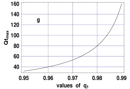
Figure 7: The dependence of $Qt_{m}$ on $q_{1}$ in the case of subcritical evolution assuming that the $\nu$ is of geometric distribution.

Figure 8: Time dependence of the correlation between the numbers living and dead nodes if $\nu$ is of geometric distribution. The curves a, b, and c belong to $q_{1}$ values $0.95,\;1,$ and $1.05$, respectively.

The dependence of the covariance function

$${\bf Cov}\{\mu_{\ell}(t)\mu_{d}(t)\}={\mathcal{D}}^{(\ell,d)}(Qt,\;{\bf E}\{\nu\},\;{\bf D}^{2}\{\nu\})$$

on the time parameter $Qt$ and the expectation value as well as the variance of the $\nu$ has been calculated by assuming the $\nu$ to be of geometric distribution. Since in this case ${\bf E}\{\nu\}=q_{1}$ and ${\bf D}^{2}\{\nu\}=q_{1}(1+q_{1})$, thus one can write

$${\bf Cov}\{\mu_{\ell}(t)\mu_{d}(t)\}={\mathcal{D}}^{(\ell,d)}(Qt,q_{1}).$$

The contour plot of this covariance function has been calculated in the $(Qt,q_{1})$ plain for the subcritical values of $q_{1}$. The results are seen in Fig. 5. In order to show more precisely the form of time dependence of ${\mathcal{D}}^{(\ell,d)}(x,q_{1})$, three curves a, b, and c corresponding to the values $q_{1}=0.96,0.97$, and $0.98$, respectively, are plotted in Fig. 6. One can observe that each of the covariance curves vs. time has a well defined maximum. The time parameter $Qt_{m}$ due to the maximum of the covariance function depends rather sensitively on $q_{1}$. It is interesting to look at the variation of $Qt_{m}$ when $q_{1}\Rightarrow 1$. The curve plotted in Fig. 7 shows this variation, and one can see a steep increase of $Qt_{m}$ when $q_{1}$ is approaching to $1$.

Figure 9: Dependence of the correlation between the numbers of living and dead nodes on $q_{1}$ at time instants $Qt=100$, (a), $Qtx=500$, (b) and $Qt=\infty$, (c).

Correlation function.    It is trivial that the numbers of living and dead nodes are correlated, but the time dependence of the correlation function

$${\mathcal{C}}^{(\ell,d)}(t,q_{1},q_{2})=\frac{{\bf Cov}\{\mu_{\ell}(t)\mu_{d}(t)\}}{{\bf D}\{\mu_{\ell}(t)\}{\bf D}\{\mu_{d}(t)\}},$$ (55)

has some specific features, namely, in the case of subcritical evolution the correlation function — after a sharp increase — is converging to zero when $Qt\Rightarrow\infty$, while in the case of supercritical evolution reaching rapidly the value $1$.

If the random evolution is critical, i.e. $q_{1}=1$, then we have

$${\mathcal{C}}^{(\ell,d)}(t,1,q_{2})=\frac{\sqrt{3}}{2}\;\left[1+\frac{3}{{\bf D}^{2}\{\nu\}\;(Qt)^{2}}\right]^{-1/2},$$ (56)

which shows that the limit value of the correlation

$$\lim_{Qt\rightarrow\infty}\;{\mathcal{C}}^{(\ell,d)}(t,1,q_{2})=\frac{\sqrt{3}}{2}$$ (57)

is independent of distributions of $\nu$ and $\tau$. This very important limit law expresses the fact that the relation between the numbers of living and dead nodes near the critical state, and at time moments sufficiently far from the beginning of the process, becomes almost independent of rules controlling the evolution.

Fig. 8   illustrates the time dependence   of the correlation function $\;\;{\mathcal{C}}^{(\ell,d)}(t,q_{1},q_{2})$ in the case if $\nu$ is of geometric distribution. The curves a, b, and c belong to the $q_{1}$ values $0.95,\;1,$ and $1.05$, respectively. It can be shown that these curves are rather insensitive to the distribution of $\nu$.

It seems to be worthwhile to present some curves reflecting the dependence of ${\mathcal{C}}^{(\ell,d)}(t,q_{1},q_{2})$ on $q_{1}$ at different time instants. In Fig. 9 we can see that the transition of the correlation function from $0$ to $1$ becomes sharper and sharper with increasing $Qt$. The curves a and b are belonging to the time parameters $Qt=100$ and $Qt=500$, respectively, while the curve c shows how the correlation function depends on $q_{1}$ at $Qt=\infty$. One has to note that

$$\lim_{Qt\rightarrow\infty}{\mathcal{C}}^{(\ell,d)}(t,1+\epsilon,q_{2})=\left\{\begin{array}[]{ll}0,&\mbox{if $\epsilon<0$,}\\ \mbox{ }&\mbox{ }\\ \sqrt{3}/2,&\mbox{if $\epsilon=0$,}\\ \\ \mbox{ }&\mbox{ }\\ 1,&\mbox{if $\epsilon>0$.}\end{array}\right.$$

4.2.2 Living nodes and lines

In order to study the time dependence of correlation between the numbers of living nodes and lines in randomly evolving trees we should calculate the expectation value

$${\bf E}\{\mu_{\ell}(t)\;\mu_{e}(t)\}=m_{1,1}^{(\ell,e)}(t),$$

which can be determined from the generating function $g^{(\ell,e)}(t,z_{\ell},z_{e})$ defined by (21). Since

$$m_{1,1}^{(\ell,e)}(t)=\left[\frac{\partial^{2}g^{(\ell,e)}(t,z_{\ell},z_{e})}{\partial z_{\ell}\;\partial z_{e}}\right]_{z_{\ell}=z_{e}=1},$$

one obtains from Eq. (22) the integral equation

$$m_{1,1}^{(\ell,e)}(t)=Q\;q_{1}\;\int_{0}^{t}e^{-Q(t-t^{\prime})}\;m_{1,1}^{(\ell,e)}(t^{\prime})\;dt^{\prime}+$$

$$Q\;\int_{0}^{t}e^{-Q(t-t^{\prime})}\;m_{1}^{(\ell)}(t^{\prime})\left\{q_{1}+q_{2}\left[1+m_{1}^{(e)}(t^{\prime})\right]\right\}\;dt^{\prime}.$$ (58)

Taking into account Eqs.

$$m_{1}^{(\ell)}(t)=e^{-(1-q_{1})Qt}$$

and

$$m_{1}^{(e)}(t)=\left\{\begin{array}[]{ll}\frac{q_{1}}{1-q_{1}}\;[1-e^{-(1-q_{1})Qt}],&\mbox{if $q_{1}\neq 1$,}\\ \mbox{ }&\mbox{ }\\ Qt,&\mbox{if $q_{1}=1$,}\end{array}\right.$$

it can be shown that the solution of (58) has the following form:

$$m_{1,1}^{(\ell,e)}(t)=\frac{{\bf D}^{2}\{\nu\}}{1-q_{1}}\;Qt\;e^{-\alpha t}-q_{2}\;\frac{q_{1}}{(1-q_{1})^{2}}\;e^{-\alpha t}(1-e^{-\alpha t}),$$ (59)

$$\mbox{if}\;\;\;\;\;\;q_{1}\neq 1,$$

where $\alpha=(1-q_{1})Q$, and

$$m_{1,1}^{(\ell,e)}(t)=(1+q_{2})\;Qt+\frac{1}{2}\;q_{2}\;(Qt)^{2},\;\;\;\;\;\;\mbox{if}\;\;\;\;\;\;q_{1}=1.$$ (60)

By using the relation

$${\bf Cov}\{\mu_{\ell}(t)\;\mu_{e}(t)\}=m_{1,1}^{(\ell,e)}(t)-m_{1}^{(\ell)}(t)\;m_{1}^{(e)}(t)$$

one can obtain that

$${\bf Cov}\{\mu_{\ell}(t)\;\mu_{e}(t)\}=\frac{{\bf D}^{2}\{\nu\}}{1-q_{1}}\;Qt\;e^{-\alpha t}-q_{1}\left[1+\frac{{\bf D}^{2}\{\nu\}}{(1-q_{1})^{2}}\right]\;e^{-\alpha t}(1-e^{-\alpha t}),$$ (61)

$$\mbox{if}\;\;\;\;\;\;q_{1}\neq 1,$$

and

$${\bf Cov}\{\mu_{\ell}(t)\;\mu_{e}(t)\}={\bf D}^{2}\{\nu\}\;Qt\left(1+\frac{1}{2}\;Qt\right),$$ (62)

$$\mbox{if}\;\;\;\;\;\;q_{1}=1.$$

Figure 10: Time dependence of the correlation between the numbers of lines and living nodes in the case when $\nu$ is of geometric distribution. The curves a, b, and c are belonging to the $q_{1}$ values $0.95,\;1,$ and $1.05$, respectively.

Let us investigate the time dependence of the correlation function

$${\mathcal{C}}^{(\ell,e)}(t,q_{1},q_{2})=\frac{{\bf Cov}\{\mu_{\ell}(t)\mu_{e}(t)\}}{{\bf D}\{\mu_{\ell}(t)\}{\bf D}\{\mu_{e}(t)\}}.$$ (63)

It can be proved that

$${\bf D}\{\mu_{e}(t)\}={\bf D}\{\mu(t)\},$$ (64)

and thus, if $q_{1}\neq 1$ then there is an easy task to calculate (63) by using the expressions (61), (29) and (64), while if $q_{1}=1$ then we can write

$${\mathcal{C}}^{(\ell,e)}(t,1,q_{2})=\frac{\sqrt{3}}{2}\;\frac{1+2\;(Qt)^{-1}}{\left[1+3\;(Qt)^{-1}\left(1+\frac{1+{\bf D^{2}}\{\nu\}}{{\bf D}^{2}\{\nu\}}\;(Qt)^{-1}\right)\right]^{1/2}},$$ (65)

from that it follows the limit relation

$$\lim_{Qt\rightarrow\infty}{\mathcal{C}}^{(\ell,e)}(t,1,q_{2})=\frac{\sqrt{3}}{2},$$

which is the same as $\lim_{t\rightarrow\infty}{\mathcal{C}}^{(\ell,d)}(t,1,q_{2})$ and so, we can conclude that the limit value of the correlation between the numbers of lines and living nodes is completely independent of the parameters determining the tree evolution process.

Fig. 10 shows the time dependence of the correlation ${\mathcal{C}}^{(\ell,e)}(t,q_{1},q_{2})$ near the beginning of the process at the values of $q_{1}=0.95,1,1.05$ assuming that $\nu$ has geometric distribution. The curve a corresponding to the subcritical evolution has a well defined maximum, and after that it decreases rapidly to zero when $t\Rightarrow\infty$. In the case of the critical evolution, i.e., when $q_{1}=1$, the correlation function passing its maximum converges to the limit value $\sqrt{3}/2$ as seen on the curve b. Finally, one can see that the curve c due to the value $q_{1}=1.05$ is reaching the level $1$ not monotonously but through a slight maximum. The dependence of the correlation function ${\mathcal{C}}^{(\ell,e)}(t,q_{1},q_{2})$ on $q_{1}$ is similar to that of ${\mathcal{C}}^{(\ell,d)}(t,q_{1},q_{2})$, i.e., the transition from $0$ to $1$ becomes sharper and sharper with increasing $Qt$.

5 Concluding remarks

By introducing the notions of living and dead nodes a new model of random tree evolution with continuous time parameter has been constructed . In order to describe the evolution process two basic random functions $\mu_{\ell}(t)$ and $\mu_{d}(t)$ have been used. The first is the actual number of living nodes, while the second that of the dead nodes at time instant $t\geq 0$.

Having assumed the evolution process to be controlled by the lifetime and the offspring number of living nodes we derived exact equations for generating functions of $\mu_{\ell}(t),\;\;\mu_{d}(t),\;\;\{\mu_{\ell}(t),\mu_{d}(t)\}$ etc., provided that at $t=0$ the tree consisted of a single living node only. It is remarkable that the average lifetime has a role of scaling the time only in these equations.

The time dependence of the average number of nodes has been used for characterization of the evolution which can be either subcritical or critical, or supercritical. It has been proved that the relative variance of the tree size is increasing with time, ie. at large $t$ the average tree size is hardly informative. If the average offspring number converges to $1$, then it has been found that the limit value of the relative variance tends to infinity.

A specific property of the tree evolution has been discovered, namely, it has been proved that the correlation between the numbers of living and dead nodes decreases to zero in subcritical and increases to $1$ in supercritical evolution, if the time parameter $Qt$ tends to infinity, but in the case of exactly critical evolution it converges to a fixed value $\sqrt{3}/2$ which is free of the parameters of the process.

References

• [1] R. Albert and A.-L. Barabรกsi, Statistical Mechanics of Complex Networks, cond-mat/0106096
• [2] S.N. Dorogovtsev and J.F. Mendes, Evolution of Random Networks, cond-mat/0106144
• [3] P. Erdรถs and A. Rรฉnyi, Publicationes Mathematicea 6 (1959) 290
• [4] P. Erdรถs and A. Rรฉnyi, Math. Inst. Hung. Acsad. 5 (1960) 17
• [5] P. Erdรถs and A. Rรฉnyi, Bull. Int. Stat. Inst, 38 (1961) 343
• [6] D.J. Watts and S.H. Strogatz, Nature 393 (1998) 440
• [7] D.J. Watts, The Dynamics of Networks Between Order and Randomness (Princeton University Press, Princeton New-Jersey, 1999)
• [8] M.E. Newman, C. Moore, and D.J. Watts, Phys. Rev. Lett. 84 (2000) 3201
• [9] A. Barabรกsi, R. Albert, and H. Jeong, Phisica A 272 (1999) 173
• [10] P.L. Krapivsky, S. Redner, and L. Leyvraz, Phys. Rev. Lett. 85 (2000) 4629
• [11] S.N. Dorogovtsev, J.F. Mendes and A. Samukhin, cond-mat/0004434
• [12] T.E. Harris, The theory of Branching Processes (Springer-Verlag, Berlin-Gรถttingen-Heidelberg, 1963)
• [13] R. Lyons and Y. Peres, Probability on Trees and Networks, (Cambridge University Press, in preparation, Current version available at http:/www. math. washington.edu/ย ejpecp/)
• [14] B. Sewastjanow, Verzweigungsprozesse (Akademie-Verlag, Berlin, 1974)
• [15] L. Pรกl, The Foundation of the Probability Calculus and Statistics (Akadรฉmiai Kiadรณ, Budapest, 1995)
• [16] L. Pรกl, Properties of Generating Functions (Internal Report, Budapest, 1994)