Chapter 0 The Architecture of Complex Systems

Vito Latora¹ and Massimo Marchiori²
1) Dipartimento di Fisica e Astronomia, Università di Catania, and INFN sezione di Catania, Catania, Italy
2) W3C and Lab. for Computer Science, Massachusetts Institute of Technology, Cambridge, USA

The Architecture of Complex Systems

1 Introduction

At the present time, the most commonly accepted definition of a complex system is that of a system containing many interdependent constituents which interact nonlinearly . Therefore, when we want to model a complex system, the first issue has to do with the connectivity properties of its network, the architecture of the wirings between the constituents. In fact, we have recently learned that the network structure can be as important as the nonlinear interactions between elements, and an accurate description of the coupling architecture and a characterization of the structural properties of the network can be of fundamental importance also to understand the dynamics of the system.

In the last few years the research on networks has taken different directions producing rather unexpected and important results. Researchers have: 1) proposed various global variables to describe and characterize the properties of real-world networks; 2) developed different models to simulate the formation and the growth of networks as the ones found in the real world. The results obtained can be summed up by saying that statistical physics has been able to capture the structure of many diverse systems within a few common frameworks, though these common frameworks are very different from the regular array, or the random connectivity, previously used to model the network of a complex system.

Here we present a list of some of the global quantities introduced to characterize a network: the characteristic path length $L$, the clustering coefficient $C$, the global efficiency $E_{\rm glob}$, the local efficiency $E_{\rm loc}$, the cost $Cost$, and the degree distribution $P(k)$. We also review two classes of networks proposed: small-world and scale-free networks. We conclude with a possible application of the nonextensive thermodynamics formalism to describe scale-free networks.

2 SMALL-WORLD NETWORKS

In ref. [16] Watts and Strogatz have shown that the connection topology of some biological, social and technological networks is neither completely regular nor completely random. These networks, that are somehow in between regular and random networks, have been named small worlds in analogy with the small world phenomenon empirically observed in social systems more than 30 years ago [12, 13]. In the mathematical formalism developed by Watts and Strogatz a generic network is represented as an unweighted graph $\bf G$ with $N$ nodes (vertices) and $K$ edges (links) between nodes. Such a graph is described by the adjacency matrix $\{a_{ij}\}$, whose entry $a_{ij}$ is either $1$ if there is an edge joining vertex $i$ to vertex $j$, and $0$ otherwise. The mathematical characterization of the small-world behavior is based on the evaluation of two quantities, the characteristic path length $L$ and the clustering coefficient $C$.

1 The characteristic path length

The characteristic path length $L$ measures the typical separation between two generic nodes of a graph $\bf G$. $L$ is defined as:

$$L({\bf G})=\frac{1}{N(N-1)}\sum_{i\neq j\in{\bf G}}d_{ij}$$

where $d_{ij}$ is the shortest path length between $i$ and $j$, i.e. the minimum number of edges traversed to get from a vertex $i$ to another vertex $j$. By definition $d_{ij}\geq 1$, and $d_{ij}=1$ if there exists a direct link between $i$ and $j$. Notice that if $\bf G$ is connected, i.e. there exists at least one path connecting any couple of vertices with a finite number of steps, then $d_{ij}$ is finite $\forall i\neq j$ and also $L$ is a finite number. For a non-connected graph, $L$ is an ill-defined quantity, because it can diverge. This problem is avoided by using $E_{\rm glob}$ in place of $L$.

2 The clustering coefficient

The clustering coefficient $C$ is a local quantity of ${\bf G}$ measuring the average cliquishness of a node. For any node $i$, the subgraph of neighbors of $i$, $\bf G_{i}$ is considered. If the degree of $i$, i. e.  the number of edges incident with $i$, is equal to $k_{i}$, then $\bf G_{i}$ is made of $k_{i}$ nodes and at most $k_{i}(k_{i}-1)/2$ edges. $C_{i}$ is the fraction of these edges that actually exist, and $C$ is the average value of $C_{i}$ all over the network (by definition $0\leq C\leq 1$):

$$C({\bf G})=\frac{1}{N}\sum_{i\in{\bf G}}C_{i}~{}~{}~{}~{}~{}~{}~{}~{}C_{i}={\mbox{ \# of edges in $\bf G_{i}$ }\over\mbox{ $k_{i}(k_{i}-1)/2$ }}$$

The mathematical characterization of the small-world behavior proposed by Watts and Strogatz is based on the evaluation of $L$ and $C$: small-world networks have high $C$ like regular lattices, and short $L$ like random graphs. The small-world behavior is ubiquitios in nature and in man-made systems. Neural networks, social systems [7] as the collaboration graph of movie actors [16] or the collaboration network of scientists [14], technological networks as the World Wide Web or the electrical power grid of the Western US, are only few of such examples. To give an idea of the numbers obtained we consider the simplest case of the neural networks investigated, that of the C. elegans: this network, represented by a graph with $N=282$ nodes (neurons) and $K=1974$ edges (connections between neurons), gives $L=2.65$ and $C=0.28$ [16]. It is also important to notice that a network as the electrical power grid of the western US, can be studied by such a formalism only if considered as an unweighted graph, i.e. when no importance whatsoever is given to the physical length of the links.

3 EFFICIENT AND ECONOMIC BEHAVIOR

A more general formalism, valid both for unweighted and weighted graphs (also non-connected), extends the application of the small-world analysis to any real complex network, in particular to those systems where the euclidian distance between vertices is important (as in the case of the electrical power grid of western US), and therefore too poorly described only by the topology of connections [8, 9]. Such systems are better described by two matrices, the adjacency matrix $\{a_{ij}\}$ defined as before, and a second matrix $\{\ell_{ij}\}$ containing the weights associated to each link. The latter is named the matrix of physical distances, because the numbers $\ell_{ij}$ can be imagined as the euclidean distances between $i$ and $j$. The mathematical characterization of the network is based on the evaluation of two quantities, the global and the local efficiency (replacing $L$ and $C$), and a third one quantifying the cost of the network. Small worlds are networks that exchange information very efficiently both on a global and on a local scale [8].

1 The global efficiency

In the case of a weighted network the shortest path length $d_{ij}$ is defined as the smallest sum of the physical distances throughout all the possible paths in the graph from $i$ to $j$ . The efficiency $\epsilon_{ij}$ in the communication between vertex $i$ and $j$ is assumed to be inversely proportional to the shortest path length: $\epsilon_{ij}=1/d_{ij}$. When there is no path in the graph between $i$ and $j$, $d_{ij}=+\infty$ and consistently $\epsilon_{ij}=0$. Suppose now that every vertex sends information along the network, through its edges. The global efficiency of $\bf G$ can be defined as an average of $\epsilon_{ij}$:

$$E_{\rm glob}({\bf G})=\frac{{{\sum_{{i\neq j\in{\bf G}}}}\epsilon_{ij}}}{N(N-1)}=\frac{1}{N(N-1)}{\sum_{{i\neq j\in{\bf G}}}\frac{1}{d_{ij}}}$$

Such a quantity is always a finite number (even when ${\bf G}$ is unconnected) and can be normalized to vary in the range $[0,1]$ if divided by $E_{\rm glob}({\bf G^{ideal}})=\frac{1}{N(N-1)}{\sum_{{i\neq j\in{\bf G}}}\frac{1}{l_{ij}}}$ , the efficiency of the ideal case ${\bf{G^{ideal}}}$ in which the graph has all the $N(N-1)/2$ possible edges. In such a case the information is propagated in the most efficient way since $d_{ij}=\ell_{ij}~{}\forall i,j$.

2 The local efficiency

One of the advantages of the efficiency-based formalism is that a single measure, the efficiency $E$ (instead of the two different measures $L$ and $C$) is sufficient to define the small-world behavior. In fact the efficiency, can be evaluated for any subgraph of $\bf G$, in particular for $\bf{G_{i}}$, the subgraph of the neighbors of $i$ (made by $k_{i}$ nodes and at most ${k_{i}(k_{i}-1)}/2$ edges), and therefore it can be used also to characterize the local properties of the graph. The local efficiency of $\bf G$ is defined as:

$$E_{\rm loc}({\bf G})=\frac{1}{N}\sum_{i\in{\bf G}}~{}{E(\bf{G_{i}})}~{}~{}~{}~{}~{}~{}~{}{E(\bf{G_{i}})}=\frac{1}{k_{i}(k_{i}-1)}{\sum_{{l\neq m\in{{\bf G_{i}}}}}\frac{1}{d^{\prime}_{lm}}}$$

where the quantities $\{d^{\prime}_{lm}\}$ are the shortest distances between nodes $l$ and $m$ calculated on the graph $\bf G_{i}$. Similarly to $E_{\rm glob}$, also $E_{\rm loc}$ can be normalized to vary in the range $[0,1]$ and plays a role similar to that of $C$ [9]. Small worlds are networks with high $E_{\rm glob}$ and high $E_{\rm loc}$.

3 The Cost

An important variable to consider, especially when we deal with weighted networks and when we want to analyze and compare different real systems, is the cost of a network [9]. In fact, we expect both $E_{\rm glob}$ and $E_{\rm loc}$ to be higher ($L$ lower and $C$ higher) as the number of edges in the graph increases. As a counterpart, in any real network there is a price to pay for number and length (weight) of edges. This can be taken into account by defining the cost of the graph $\bf G$ as the total length of the network’s wirings:

$$Cost({\bf G})=\frac{\sum_{{i\neq j\in{\bf G}}}a_{ij}~{}\ell_{ij}}{\sum_{{i\neq j\in{\bf G}}}{\ell_{ij}}}$$ (1)

Since the cost of ${\bf G}^{ideal}$ is already included in the denominator of the formula above, $Cost$ varies in $[0,1]$ and assumes the maximum value $1$ when all the edges are present in the graph. In the case of an unweighted graph, $Cost({\bf G})$ reduces to the normalized number of edges $2K/N(N-1)$.

With the three variables $E_{\rm glob}$, $E_{\rm loc}$ and $Cost$, all defined in $[0,1]$, it is possible to study in an unified way unweighted (topological) and weighted networks. And it is possible to define an economic small world as a network having low $Cost$ and high $E_{\rm loc}$ and $E_{\rm glob}$ (i.e., both economic and small-world). In figure we report an useful illustrative example obtained by means of a simple model to construct a class of weighted graphs. We start by considering a regular network of $N=1000$ nodes placed on a circle ($\ell_{i,j}$ is given by the euclidean distance between $i$ and $j$) and $K=1500$ links. A random rewiring procedure is implemented: it consists in going through each of the links in turn and independently with some probability $p$ rewire it. Rewiring means shifting one end of the edge to a new node chosen randomly with a uniform probability. In this way it is possible to tune $\bf G$ in a continuous manner from a regular lattice ($p=0$) into a random graph ($p=1$), without altering the average number of neighbors equal to $k=2K/N$. For $p\sim 0.02-0.04$ we observe the small-world behavior: $E_{\rm glob}$ has almost reached its maximum value $0.62$ while $E_{\rm loc}$ has not changed much from the maximum value $0.2$ (assumed at $p=0$). Moreover for these values of $p$ the network is also economic, in fact the $Cost$ stays very close to the minimum possible value (assumed of course in the regular case $p=0$).

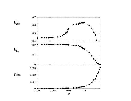
Figure 1: The three quantities $E_{\rm glob}$, $E_{\rm loc}$ and $Cost$ are reported as function of the rewiring probability $p$ for the model discussed in the text. The economic small-world behavior shows up for $p\sim 0.02-0.04$

Some examples of applications to real networks. The neural network of the C. elegans has $E_{\rm glob}=0.35$, $E_{\rm loc}=0.34$, $Cost=0.18$: the C. elegans is an economic small world because it achieves high efficiency both at the global and local level (about $35\%$ of the global and local efficiency of the ideal completely connected case); all of this at a relatively low cost, with only the $18\%$ of the wirings of the ideal graph. As a second example we consider a technological network, the MBTA, the Boston underground transportation system. The MBTA is a weighted network consisting of $N=124$ stations and $K=124$ tunnels connecting couples of stations. For such a system we obtain $E_{\rm glob}=0.63$, $E_{\rm loc}=0.03$ and $Cost=0.002$. This means that MBTA achieves the $63\%$ of the efficiency of the ideal subway with a cost of only the $0.2\%$. The price to pay for such low-cost high global efficiency is the lack of local efficiency. In fact, $E_{\rm loc}=0.03$ indicates that, differently from a neural network (or from a social system), the MBTA is not fault tolerant, i.e. a damage in a station will dramatically affect the efficiency in the connection between the previous and the next station. The difference with respect to neural networks comes from different needs and priorities in the construction and evolution mechanism. When a subway system is built, the priority is given to the achievement of global efficiency at a relatively low cost, and not to fault tolerance. In fact a temporary problem in a station can be solved in an economic way by other means: for example, walking, or taking a bus from the previous to the next station. Applications to other real networks can be found in ref.[9].

4 SCALE-FREE NETWORKS

1 Degree Distribution

Other important information on a network can be extracted from its degree distribution $P(k)$. The latter is defined as the probability of finding nodes with $k$ links: $P(k)=\frac{N(k)}{N}$, where $N(k)$ is the number of nodes with $k$ links. Many large networks, as the World Wide Web, the Internet, metabolic and protein networks have been named scale-free networks because their degree distribution follows a power-law for large $k$ [2, 3]. Also a social system of interest for the spreading of sexually transmitted diseases [11], and the connectivity network of atomic clusters’ systems [6] show a similar behavior. The most interesting fact is that neither regular nor random graphs display long tails in P(k), and the presence of nodes with large $k$ strongly affects the properties of the network [15], as for instance its response to external factors [5]. In ref.[2] Barabasi and Albert have proposed a simple model (the BA model) to reproduce the P(k) found in real networks by modelling the dynamical growth of the network. The model is based on two simple mechanisms, growth and preferential attachment, that are also the main ingredients present in the dynamical evolution of the real-world networks. As an example, the World Wide Web grows in time by the addition of new web pages, and a new web page will more likely include hyperlinks to popular documents with already high degree. Starting by an initial network with a few nodes and adding new nodes with new links preferentially connected to the most important existing nodes, the dynamics of the BA model produces (in the stationary regime) scale-free networks with a power-law degree distribution [2]:

$$P(k)\sim k^{-\gamma}~{}~{}~{}\gamma=3$$

The model predicts the emergence of the scale-free behavior observed in real networks, though the exponents in the power law of real networks can be different from 3 (usually it is in the range between 2 and 3).

2 Nonextensive Statistical Mechanics

A more careful analysis of the shape of P(k) of many of the real networks considered evidentiates the presence of a plateau for small k. See for example fig.1a of Ref.[2] and fig.2b of Ref. [11]. We have observed that such a plateau for small $k$ and the different slopes of the power-law for large $k$ can be perfectly reproduced by using the generalized power-law distribution

$$P(k)\sim[1+(q-1)\beta k]^{\frac{1}{1-q}}$$

with two fitting parameters: $q$ related to the slope of the power law for large $k$, and $\beta$ [4]. The generalized probability distribution above can be obtained as a stationary solution of a generalized Fokker-Planck equation with a nonlinear diffusion term [10]. We therefore believe that is possible to rephrase the generalized Fokker-Planck equation in terms of a generalized mechanism of network construction, and to implement a model (more general than the BA model) able to reproduce the plateau and the different slopes of P(k).

ACKNOWLEDGMENTS

We thank E. Borges, P. Crucitti, M.E.J. Newman, A. Rapisarda, C. Tsallis and G. West for their useful comments.

References

- [1] Baranger, M. “Chaos, Complexity, and Entropy: a Physics Talk for Non-Physicists.” http://www.necsi.org/projects/baranger/cce.html
- [2] Barabási, A.-L., and R. Albert. “Emergence of Scaling in Random Networks.” Science 286, (1999):509-512.
- [3] Jeong, H., B. Tombor, R. Albert, Z. N. Oltvai and A.-L. Barabási. “The Large-Scale Organization of Metabolic Networks.” Nature 407, (2000):651-654.
- [4] Borges, E., V. Latora, A. Rapisarda and C. Tsallis. In preparation.
- [5] Crucitti, P., V. Latora, M. Marchiori, and A. Rapisarda. “Efficiency of Scale-Free Networks: Error and Attack Tolerance.” cond-mat/0205601.
- [6] Doye, J.P.K. “The network topology of a potential energy landscape: A static scale-free network.” cond-mat/0201430.
- [7] Girvan, M., and M. E. J. Newman. “Community structure in social and biological networks” cond-mat/0112110.
- [8] Latora, V., and M. Marchiori. “Efficient Behavior of Small-World Networks.” Phys. Rev. Lett. 87, (2001):198701.
- [9] Latora, V., and M. Marchiori. “Economic Small-World Behavior in Weighted Networks.” cond-mat/0204089.
- [10] Plastino, A.R., and A. Plastino. “Nonextensive statistical mechanics and generalized Fokker-Planck equation.” Physica A222, (1995):347-354.
- [11] Liljeros, F. L., C. R. Edling, N. Amaral, H. E. Stanley, and Y. Aberg. “The Web of Human Sexual Contacts.” Nature 411, (2001):907-908
- [12] Milgram, S. “The Small World Problem.” Psychol. Today, 2, (1967):60-67.
- [13] Newman, M. E. J. “Models of the small world.” J. Stat. Phys., 101, (2000):819-841.
- [14] Newman, M. E. J. “Scientific collaboration networks. ” Phys. Rev. E64, (2001) 016131 and Phys. Rev. E64, (2001) 016132.
- [15] Pastor-Satorras R., and A. Vespignani. “Epidemic Spreading in Scale-Free Networks.” Phys. Rev. Lett. 86, (2001):3200-3203.
- [16] Watts, D. J., and S. H. Strogatz. “Collective Dynamics of Small-World Networks.” Nature 393, (1998): 440-442.