Theory of Excitonic States in CaB₆

Abstract

We study the excitonic states in CaB₆ in terms of the Ginzburg-Landau theory. By minimizing the free energy and by comparing with experimental results, we identify two possible ground states with exciton condensation. They both break time-reversal and inversion symmetries. This leads to various magnetic and optical properties. As for magnetic properties, it is expected to be an antiferromagnet, and its spin structure is predicted. It will exhibit the magnetoelectric effect, and observed novel ferromagnetism in doped samples and in thin-film and powder samples can arise from this effect. Interesting optical phenomena such as the nonreciprocal optical effect and the second harmonic generation are predicted. Their measurement for CaB₆ will clarify whether exciton condensation occurs or not and which of the two states is realized.

I Introduction

CaB₆ and its doped system Ca_1-xLa_xB₆ have been the subject of intensive studies since the discovery of “high temperature ferromagnetism” young . The understanding of the parent compound CaB₆, which we focus in this paper, is essential to that of this novel ferromagnetism. This ferromagnetism is peculiar in some respects: (i) the Curie temperature ($\sim 600{\rm K}$) is high in spite of a small moment (0.07$\mu_{\rm B}$/La), (ii) it occurs only in a narrow doping range ($x<0.01$), and (iii) there are no partially filled $d$- or $f$-bands. Soon after this discovery, two scenarios are proposed; one is based on a ferromagnetic phase of a dilute electron gas ceperley , and another is based on an excitonic state zra ; bv where the doped carriers are concluded to be fully spin-polarized vkr . Earlier band structure calculations hy ; mcpm found the small overlap of the conduction and valence bands near the three X-points. In the de Haas-van Alphen measurement, the Fermi surfaces of both electrons and holes are observed hall , which confirms the smallness of the gap. Furthermore, the symmetry of the wave function at the bottom of conduction band (the top of the valence band) forbids a finite dipole matrix elements. Therefore the dielectric constant is not enhanced even when the band gap is reduced hr , and the excitonic instability is not suppressed; CaB₆ can thus be regarded as a promising candidate for the excitonic state. A recent band calculation based on GW approximation tromp , on the other hand, predicts a large band gap of $\sim$ 0.8 eV, which is too large compared with the exciton binding energy of the order of $T_{c}\sim 600{\rm K}$. Measurements on photoemission ARPES and soft X-ray emission Xray observed a band gap of $\sim$ 1 eV, consistent with this GW calculation; yet a surface effect in photoemission should be seriously considered before any conclusion is drawn. Particularly, another GW calculation kino found the small overlap similar to the LDA calculation. Furthermore, there are several experimental evidences showing a symmetry breaking with magnetism below $T_{c}\sim 600$K . X-ray diffraction and Raman scattering experiments udagawa shows an anomaly at $T_{c}\sim 600$K, below which the symmetry is lowered from cubic to tetragonal. A $\mu$SR measurement ohishi detected an internal magnetic field, which suggests an existence of a magnetic moment.

These findings contradict the large band gap because any instabilities are unlikely if that is the case. In addition, sensitivity to impurities and defects suggests a small band gap/overlap. Thus, it seems likely that the exciton condensation occurs in this compound due to a small band gap/overlap. One can then attribute the high Curie temperature in Ca_1-xLa_xB₆ to the excitonic instability in the parent compound, which is determined by the exciton binding energy. Nonetheless, even if we assume the exciton condensation, there remain many mysteries. The peculiarity of ferromagnetism in Ca_1-xLa_xB₆ reveals itself in the strong sample dependence. In Ref. zra, , the doped carriers are assumed to be essential to ferromagnetism, but recent experiments could not find the correlation between the transport properties and magnetism. The smallness of the magnetic moment ($\sim 0.07\mu_{B}/$La) is not fully accounted for, although numerous attempts have been made zra ; bg ; b ; vb ; bbm . Moreover deficiency in Ca sites morikawa or doping of divalent elements such as Ba young or Sr ott also induces ferromagnetism. Another hint is that the ferromagnetic moment is enhanced in the thin-film sample terashima , or near the surface from electron spin resonance (ESR) kunii . This fact suggests that some kind of symmetry lowering is related to the ferromagnetism.

Because of this controversial situation, it is worthwhile to give solid theoretical results which are independent of the details of microscopic models. In this paper we deal with this problem from the viewpoint of symmetry. The only assumption we take as the basis of our analysis is that the parent compound CaB₆ is a triplet excitonic insulator with the order parameters made from the ${\rm X}^{\prime}_{3}$- (conduction band) and X₃- (valence band) wavefunctions at X-points. The analysis based on the Ginzburg-Landau expansion becomes exact by considering the symmetry properties of the order parameters. All possible states are classified according to the irreducible representation of the magnetic point group. We can then predict many nontrivial physical properties for each of the states, which can be tested experimentally. Most important of these are that these states break both the time reversal $(R)$ and space inversion $(I)$ symmetries, while their product $RI$ remains intact. This implies that CaB₆ is an antiferromagnet (AF). This also leads to the magneto-electric (ME) effect; namely the ferromagnetic moment is induced when the electric field is applied or the electric polarization is induced when the magnetic field is applied. This offers a new mechanism of the novel ferromagnetism in Ca_1-xLa_xB₆, i.e. ferromagnetism is induced near impurities or surfaces by the ME effect We note that the present theory of ferromagnetism is different from those in Ref. zra, ; bv, , though all these theories assume exciton condensation. The relation between our theory and the theories in Ref. zra, ; bv, is presented in detail in the last section. We have published a short version msnm of this paper, but this paper contains new results such as a pattern of the magnetic moments, and optical properties, as well as full and detailed description of the discussion. The plan of this paper is as follows. In Section II, the excitonic order parameters are defined and the Ginzburg-Landau expansion is developed in III. Physical properties of each state is described in Section IV, and V is devoted to discussions and conclusions.

Here we remark a role of spin-orbit coupling. In subsequent discussions we take into account the spin-orbit coupling. Its presence is crucial in our analysis by the GL theory. Limit of zero spin-orbit coupling is discussed in Appendix D, and it can be contrasted with the nonzero case. In our numerical estimation for coefficients in GL free energy (Fig. 2), we neglected the spin-orbit coupling, because it greatly simplifies the calculation; in interpreting its results, however, we should keep in mind that we are always treating the case of nonzero spin-orbit coupling.

II Excitonic Order Parameters

Let $b_{\bm{k}\sigma}$ and $a_{\bm{k}\sigma}$ denote annihilation operators of electrons with spin $\sigma$ at the conduction and the valence bands respectively hr . When excitons are formed, excitonic order parameters $\langle b_{\bm{k}\alpha}^{\dagger}a_{\bm{k^{\prime}}\beta}\rangle$ will have nonzero values. Excitonic instability occurs only in the vicinity of the X points hy ; mcpm , i.e. $\bm{Q}_{x}=(\pi,0,0),\ \bm{Q}_{y}=(0,\pi,0),\ \bm{Q}_{z}=(0,0,\pi)$ in the cubic Brillouin zone, where the conduction and the valence bands approach each other with a small overlap/gap. We make the following assumptions;

1. The order parameters are $\bm{k}$-independent near the X points.

2. The order parameters connecting different X points are neglected bv .

Consequently, we keep only the order parameters $\eta(\bm{Q}_{i})_{\alpha\beta}=\langle b_{\bm{Q}_{i}\alpha}^{\dagger}a_{\bm{Q}_{i}\beta}\rangle$ hrremark . Still we have $2\cdot 2\cdot 3=12$ complex order parameters involved and the problem is quite complicated. The GL theory is so powerful that it helps us from this difficulty. The cubic (${\rm O}_{\rm h}$) symmetry of the lattice considerably restricts the form of the GL free energy $\Phi$, as is similar in the GL theory for unconventional superconductors vg ; su . In this section and in the next section, we construct the GL free energy and discuss its mimima. The argument is rather technical, because we will make full use of the point-group symmetry to deal with the twelve complex order parameters. Readers who are not accustomed to detailed point-group discussions can jump to Section IV.

At each X point, the $\bm{k}$-group, i.e. the group which keeps $\bm{k}$ unchanged, is tetragonal (${\rm D}_{\rm 4h}$), and the conduction and the valence band states belong to ${\rm X}^{\prime}_{3}$ and ${\rm X}_{3}$ representations, respectively according to band calculation hy ; mcpm , when we take the origin as the center of a B₆ tetrahedron. In the absence of the spin-orbit coupling, the order parameter $\eta(\bm{Q}_{i})_{\alpha\beta}$ transform as a D${}_{4\text{h}}$ irreducible representation ${\rm X}_{3}\times{\rm X}_{3}^{\prime}={\rm X}^{\prime}_{1}$. From now on we shall take the spin-orbit coupling into account. Then, the representation of $\eta$ will be altered. We restrict our analysis on the triplet channel for the excitons, because the exchange interaction usually favors the triplet state compared with the singlet state zra . Then, the spin-1 representation is multiplied to $\text{X}^{\prime}_{1}$, and the triplet order parameters follow the representations ${\rm X}_{4}^{\prime}+{\rm X}_{5}^{\prime}$ in the ${\rm D}_{{\rm 4h}}$ group. Let us now construct the order parameters explicitly. We take the $\bm{Q}_{z}$ point as an example; the triplet order parameters have three components, following the spin-1 representation. By recalling that a spherical harmonics with $l=1$ is represented by $x\pm{\rm i}y,z$, we can recombine the triplet order parameters as

$$\eta_{x}(\bm{Q}_{z})=-\frac{{\rm i}}{\sqrt{2}}(\eta_{\uparrow\downarrow}(\bm{Q}_{z})+\eta_{\downarrow\uparrow}(\bm{Q}_{z})),$$ (1)

$$\eta_{y}(\bm{Q}_{z})=-\frac{{\rm 1}}{\sqrt{2}}(\eta_{\uparrow\downarrow}(\bm{Q}_{z})-\eta_{\downarrow\uparrow}(\bm{Q}_{z})),$$ (2)

$$\eta_{z}(\bm{Q}_{z})=\frac{{\rm i}}{\sqrt{2}}(\eta_{\downarrow\downarrow}(\bm{Q}_{z})-\eta_{\uparrow\uparrow}(\bm{Q}_{z})),$$ (3)

or in a short form

$$\eta_{i}(\bm{Q}_{a})=-\frac{{\rm i}}{\sqrt{2}}\sum_{\alpha,\beta}\eta_{\alpha\beta}(\bm{Q}_{a})\sigma^{i}_{\alpha\beta}.$$ (4)

The reason why we introduced these linear combinations is because they are convenient for subsequent symmetry discussions. Their phase factors are chosen so that the time-reversal $R$ operates as complex conjugation $R\eta_{i}(\bm{Q}_{a})=\eta_{i}^{*}(\bm{Q}_{a})$. By investigating their transformation property under D${}_{4\text{h}}$, which transforms $\bm{Q}_{z}$ onto itself, we find that $\eta_{z}$ follows the $X^{\prime}_{4}$ representation, while $\eta_{x}$ and $\eta_{y}$ follow the $X^{\prime}_{5}$ in ${\rm D}_{{\rm 4h}}$. Here the spin-quantization axis in (1)-(3) is taken to be the $z$-axis. Since we are taking into account the spin-orbit coupling, these up- and down-spins should be interpreted as pseudospins su .

When we consider the three X points, the cubic symmetry is restored. We find that nine components of the order parameters are classified into irreducible representations of ${\rm O}_{\rm h}$ as ${\rm\Gamma}_{\rm 15}+{\rm\Gamma}_{\rm 15}+{\rm\Gamma}_{\rm 25}$, all of which are 3-dimensional. Let us call basis functions as $\eta_{i}({\rm\Gamma}_{15},1)$, $\eta_{i}({\rm\Gamma}_{15},2)$ and $\eta_{j}({\rm\Gamma}_{25})$, where $i=x,y,z$ and $j=x(y^{2}-z^{2}),y(z^{2}-x^{2}),z(x^{2}-y^{2})$. These basis functions transform like a vector $(x,y,z)$ for $\Gamma_{15}$ and like $(x(y^{2}-z^{2}),y(z^{2}-x^{2}),z(x^{2}-y^{2}))$ for $\Gamma_{25}$. The basis functions are given as

$$\eta_{z}({\rm\Gamma}_{15},1)=\eta_{z}(\bm{Q}_{z})=\frac{{\rm i}}{\sqrt{2}}(\eta_{\downarrow\downarrow}(\bm{Q}_{z})-\eta_{\uparrow\uparrow}(\bm{Q}_{z})),$$

$$\eta_{z}({\rm\Gamma}_{15},2)=\frac{1}{\sqrt{2}}(\eta_{z}(\bm{Q}_{x})+\eta_{z}(\bm{Q}_{y}))=$$

$$\makebox[2.84526pt]{}-\frac{1}{2}\{{\rm i}(\eta_{\uparrow\downarrow}(\bm{Q}_{y})+\eta_{\downarrow\uparrow}(\bm{Q}_{y}))+(\eta_{\uparrow\downarrow}(\bm{Q}_{x})-\eta_{\downarrow\uparrow}(\bm{Q}_{x}))\}\ \ \ \ \ ,$$

$$\eta_{z(x^{2}-y^{2})}({\rm\Gamma}_{25})=\frac{1}{\sqrt{2}}(\eta_{z}(\bm{Q}_{x})-\eta_{z}(\bm{Q}_{y}))=$$

$$\makebox[8.53581pt]{}\frac{1}{2}\{{\rm i}(\eta_{\uparrow\downarrow}(\bm{Q}_{y})+\eta_{\downarrow\uparrow}(\bm{Q}_{y}))-(\eta_{\uparrow\downarrow}(\bm{Q}_{x})-\eta_{\downarrow\uparrow}(\bm{Q}_{x}))\}.$$

We defined these linear combinations in order to facilitate the construction of the GL free energy $\Phi$ in the next section. Here, the spin-quantization axis in $\eta_{\alpha\beta}(\bm{Q}_{i})$ is taken as the $+i$-axis ($i=x,y,z$). Other components are obtained by cyclic permutations of $x,y,z$. It is easily shown that $I\bm{\eta}=-\bm{\eta}$, and $R\bm{\eta}=\bm{\eta}^{*}$, where we defined for brevity

$$\bm{\eta}(\Gamma_{15},1)=(\eta_{x}(\Gamma_{15},1),\eta_{y}(\Gamma_{15},1),\eta_{z}(\Gamma_{15},1)),$$

$$\bm{\eta}(\Gamma_{15},2)=(\eta_{x}(\Gamma_{15},2),\eta_{y}(\Gamma_{15},2),\eta_{z}(\Gamma_{15},2)),$$

$$\bm{\eta}(\Gamma_{25})=(\eta_{x(y^{2}-z^{2})}(\Gamma_{25}),\eta_{y(z^{2}-x^{2})}(\Gamma_{25}),$$

$$\makebox[113.81102pt]{}\eta_{z(x^{2}-y^{2})}(\Gamma_{25})).$$

III Ginzburg-Landau Theory and Determination of the Ground State

III.1 Quadratic Order Terms

Let us now write down the GL free energy in terms of these order parameters. The GL free energy $\Phi$ should be invariant under the elements of ${\rm O}_{\rm h}$ and under the time-reversal $R$. We make two remarks helpful in writing down $\Phi$. First, only even-order terms in $\bm{\eta}$ are allowed by the inversion symmetry. Second, owing to the time-reversal symmetry, the order of ${\rm Im}\bm{\eta}$ in each term should be even. Thus, $\Phi$ is given up to quadratic order as

$$\Phi^{(2)}=A_{1}\sum_{i}({\rm Re}\ \eta_{i}(\Gamma_{15},1))^{2}$$

$$\makebox[1.42262pt]{}+A_{2}\sum_{i}({\rm Re}\ \eta_{i}(\Gamma_{15},2))^{2}\ \ \$$

$$\makebox[1.42262pt]{}+A_{3}\sum_{i}{\rm Re}\ \eta_{i}(\Gamma_{15},1){\rm Re}\ \eta_{i}(\Gamma_{15},2)$$

$$\makebox[1.42262pt]{}+A_{4}\sum_{j}({\rm Re}\ \eta_{j}(\Gamma_{25}))^{2}$$

$$\makebox[1.42262pt]{}+B_{1}\sum_{i}({\rm Im}\ \eta_{i}(\Gamma_{15},1))^{2}+B_{2}\sum_{i}({\rm Im}\ \eta_{i}(\Gamma_{15},2))^{2}$$

$$\makebox[1.42262pt]{}+B_{3}\sum_{i}{\rm Im}\ \eta_{i}(\Gamma_{15},1){\rm Im}\ \eta_{i}(\Gamma_{15},2)$$

$$\makebox[1.42262pt]{}+B_{4}\sum_{j}({\rm Im}\ \eta_{j}(\Gamma_{25}))^{2},\ \ \ \ \$$ (5)

where $A_{i},B_{i}$ are constants. As there exist no other symmetries than considered above, these $A_{i}$ and $B_{i}$ are independent parameters.

Let us determine the ground state of the system from the GL free energy. Minimizing $\Phi^{(2)}$, we find that one of the following states will be realized as the temperature is lowered;

(A) $$\text{Re}\ \bm{\eta}(\Gamma_{15},1)=c\ \text{Re}\ \bm{\eta}(\Gamma_{15},2)\neq\bm{0},$$

(B) $${\rm Re}\ \bm{\eta}(\Gamma_{25})\neq\bm{0},$$

(C) $${\rm Im}\ \bm{\eta}(\Gamma_{15},1)=c\ {\rm Im}\ \bm{\eta}(\Gamma_{15},2)\neq\bm{0},$$

(D) $${\rm Im}\ \bm{\eta}(\Gamma_{25})\neq\bm{0},$$

where $c$ is a nonzero constant. Therefore, condensations of excitons in $\Gamma_{15}$ and in $\Gamma_{25}$ do not occur simultaneously.

In all cases (A)-(D), all directions of the vector $\bm{\eta}$ are degenerate, and this degeneracy will be lifted in the quartic order terms in $\Phi$, as we shall see afterwards. All these states are accompanied by a lattice distortion. This distortion, however, is expected to be rather small, because it couples to the order parameter in the quadratic order, not linear order. Indeed, the distortion detected by the X-ray scattering is tetragonal and is as small as $0.03\%$ udagawa . This smallness of distortion is a common feature also in other hexaborides; for example, there observed no lattice distortion associated with low-temperature antiferromagnetism in GdB₆ gdb6 , and antiferroquadrupolar ordering in CeB₆ ceb6 . Ferromagnetic EuB₆ eub6 should also have a distortion away from a cubic lattice, though not observed experimentally. It is because ferromagnetism cannot occur in a cubic lattice from general symmetry argument cubic .

III.2 Microscopic Calculation for Quadratic Order Terms

To study which state is realized, we shall calculate the coefficients in $\Phi^{(2)}$ by the Hartree-Fock approximationhr , including coupling terms between the order parameters corresponding to the different X points. Because the spin-orbit coupling is weak in this compound, we shall neglect it in the following microscopic calculation.

In order to derive the quadratic term $\Phi^{(2)}$ of the GL theory for the triplet order parameters, we have only to concentrate on the following termhr .

$$-\sum_{ij=x,y,z}(\langle a_{\bm{Q}_{i}\alpha}^{\dagger}b_{\bm{Q}_{i}\beta}\rangle\delta_{\kappa,a}\delta_{\kappa^{\prime},b}+\langle b_{\bm{Q}_{i}\alpha}^{\dagger}a_{\bm{Q}_{i}\beta}\rangle\delta_{\kappa,b}\delta_{\kappa^{\prime},a})$$

$$\ \ \times V_{\bm{Q}_{j},\bm{Q}_{i}}^{\kappa\kappa^{\prime\prime\prime}\kappa^{\prime\prime}\kappa^{\prime}}\delta_{\alpha,\eta}\delta_{{\beta},{\gamma}}\times$$

$$\ \ (\langle a_{\bm{Q}_{j}\gamma}^{\dagger}b_{\bm{Q}_{j}\eta}\rangle\delta_{\kappa^{\prime\prime},a}\delta_{\kappa^{\prime\prime\prime},b}+\langle b_{\bm{Q}_{j}\gamma}^{\dagger}a_{\bm{Q}_{j}\eta}\rangle\delta_{\kappa^{\prime\prime},b}\delta_{\kappa^{\prime\prime\prime},a}),$$ (6)

where

$$V_{\bm{Q}_{j},\bm{Q}_{i}}^{\kappa\kappa^{\prime}\kappa^{\prime\prime}\kappa^{\prime\prime\prime}},$$

$$= \int{\rm d}{\bm{x}}\int{\rm d}{\bm{x}^{\prime}}\phi_{\bm{Q}_{i}}^{\kappa}(\bm{x})\phi_{\bm{Q}_{j}}^{\kappa^{\prime}}(\bm{x})\frac{e^{2}}{\epsilon|\bm{x}-\bm{x}^{\prime}|}\phi_{\bm{Q}_{j}}^{\kappa^{\prime\prime}}(\bm{x}^{\prime})\phi_{\bm{Q}_{i}}^{\kappa^{\prime\prime\prime}}(\bm{x}^{\prime}),$$

and $\epsilon$ is a dielectric constant, $\phi_{\bm{Q}_{i}}^{\kappa}(\bm{x})$ is the Bloch wavefunction of the $\kappa$-band ($\kappa=a,b$) at $\bm{k}=\bm{Q}_{i}$, taken as real. We assume that screening of Coulomb interaction is weak.

Figure 1: (A) Wavefunction of $\rm{X}_{3}^{\prime}$ from the d-orbit of the Ca-sites, $\phi_{\bm{Q}_{z},{\rm X}_{3}^{\prime}}^{\rm{Ca:d-orbit}}$ (B) Wavefunction of ${\rm X}_{3}^{\prime}$ from the p-orbits of the B-sites, $\phi_{\bm{Q}_{z},{\rm X}_{3}^{\prime}}^{\rm{B:p-orbit}}$ (C) Wavefunction of ${\rm X}_{3}$ from the p-orbits of the B-sites, $\phi_{\bm{Q}_{z},{\rm X}_{3}}^{\rm{B:p-orbit}}$. All the wavefunctions depicted in this figure have crystal momentum $\bm{Q}_{z}=(0,0,\pi)$

Let us construct the wavefunctions involved in the exciton formation. The wavefunction for the conduction band $\phi_{\bm{Q}_{i}}^{b}(\bm{x})$ at the X points mainly consists of the p-orbits of the boron ions and the d-orbits of the calcium ions. These constituent wavefunctions, $\phi_{\bm{Q}_{i},{\rm X}_{3}^{\prime}}^{\rm{B:p-orbit}}$ and $\phi_{\bm{Q}_{i},{\rm X}_{3}^{\prime}}^{\rm{Ca:d-orbit}}$, are depicted in Fig. 1 (A) (B). The wavefunction $\phi_{\bm{Q}_{i}}^{b}(x)$ is a bonding orbital of these two:

$$\phi_{\bm{Q}_{i}}^{b}(x)=c\phi_{\bm{Q}_{i},{\rm X}_{3}^{\prime}}^{\rm{B:p-orbit}}+(1-c)\phi_{\bm{Q}_{i},{\rm X}_{3}^{\prime}}^{\rm{Ca:d-orbit}}.$$ (7)

On the other hand, the wavefunction of the valence band at the X points is mainly composed of the p-orbits of the boron sites, as shown in Fig. 1 (C). As a simple estimation, we approximate the orbitals of the boron and the calcium ions as those of a hydrogen-like atom with charge $+2e$ and $+3e$, respectively. We believe that using more realistic orbitals in the solid will not change our conclusions described below. Owing to the time-reversal symmetry, the wavefunctions at each X-point can be taken as real. Still, there remains uncertainty in relative signs of the Bloch wavefunctions among the X-points. We define this as follows;

$$C_{3}^{[111]}\phi_{\bm{Q}_{z}}^{\kappa}(x) = \phi_{\bm{Q}_{x}}^{\kappa}(x),$$

$$(C_{3}^{[111]})^{2}\phi_{\bm{Q}_{z}}^{\kappa}(x) = \phi_{\bm{Q}_{y}}^{\kappa}(x),$$

where $C_{3}^{[111]}$ is a three-fold rotation around the [111] direction. This particular choice of relative signs of the wavefunctions at different X-points does not affect physical consequences given below; another choice leads to the same physical consequences.

Now we can evaluate the coefficient of eq.(5) from eq.(6). Because there are some relation such as $V_{\bm{Q}_{x},\bm{Q}_{y}}^{baba}=V_{\bm{Q}_{y},\bm{Q}_{x}}^{baba}=V_{\bm{Q}_{y},\bm{Q}_{z}}^{baba}=V_{\bm{Q}_{z},\bm{Q}_{x}}^{baba}$, we have only to evaluate three quantities $\alpha=V_{\bm{Q}_{i},\bm{Q}_{i}}^{baba}$, $\beta=V_{\bm{Q}_{x},\bm{Q}_{y}}^{baba}$, $\gamma=V_{\bm{Q}_{x},\bm{Q}_{y}}^{bbaa}$. In terms of these quantities, the coefficients in the GL free energy (5) are expressed as

$$\begin{array}[]{ll}A_{1}=C+\alpha,&A_{2}=C+\alpha+\beta-\gamma,\\ A_{3}=2\sqrt{2}(\beta-\gamma),&A_{4}=C+\alpha-\beta+\gamma,\\ B_{1}=C-\alpha,&B_{2}=C-\alpha-\beta-\gamma,\\ B_{3}=-2\sqrt{2}(\beta+\gamma),&B_{4}=C-\alpha+\beta+\gamma,\end{array}$$ (8)

where $C$ is a constant. These satisfy relations (70) in Appendix D, which reflects the SU(2) symmetry in the spin space in the limit of zero spin-orbit coupling. To determine which type of excitons will condense, we diagonalize $\Phi^{(2)}$ as

$$\Phi^{(2)} = \lambda_{+}^{\rm{Re}}|{\rm{Re}}\bm{\bm{\eta}}(\Gamma_{15},+)|^{2}+\lambda_{+}^{\rm{Im}}|{\rm{Im}}\bm{\bm{\eta}}(\Gamma_{15},+)|^{2}$$ (9)

$$+\lambda_{-}^{\rm{Re}}|{\rm{Re}}\bm{\bm{\eta}}(\Gamma_{15},-)|^{2}+\lambda_{-}^{\rm{Im}}|{\rm{Im}}\bm{\bm{\eta}}(\Gamma_{15},-)|^{2}$$

$$+\lambda_{\Gamma_{25}}^{\rm{Re}}|{\rm{Re}}\bm{\bm{\eta}}(\Gamma_{25})|^{2}+\lambda_{\Gamma_{25}}^{\rm{Im}}|{\rm{Im}}\bm{\bm{\eta}}(\Gamma_{25})|^{2},$$

where

$$\lambda_{\pm}^{\rm{Re}} = C+\frac{1}{2}(2\alpha+\beta-\gamma\pm 3(\beta-\gamma)),$$

$$\lambda_{\pm}^{\rm{Im}} = C+\frac{1}{2}(-2\alpha-\beta-\gamma\pm 3(-\beta-\gamma)),$$

$$\lambda_{\Gamma_{25}}^{\rm{Re}} = C+\alpha-\beta+\gamma=\lambda_{-}^{{\rm Re}},$$

$$\lambda_{\Gamma_{25}}^{\rm{Im}} = C-\alpha+\beta+\gamma=\lambda_{-}^{{\rm Im}},$$ (10)

and

$$\bm{\eta}(\Gamma_{15},+)=\frac{1}{\sqrt{3}}(\bm{\eta}(\Gamma_{15},1)+\sqrt{2}\bm{\eta}(\Gamma_{15},2)),$$ (11)

$$\bm{\eta}(\Gamma_{15},-)=\frac{1}{\sqrt{3}}(\sqrt{2}\bm{\eta}(\Gamma_{15},1)-\bm{\eta}(\Gamma_{15},2)).$$ (12)

The degeneracy in $\lambda_{\Gamma_{25}}^{\rm{Im}}=\lambda_{-}^{\rm{Im}}$, $\lambda_{\Gamma_{25}}^{\rm{Re}}=\lambda_{-}^{\rm{Re}}$ is a consequence of (70) which is valid in the absence of the spin-orbit coupling; this degeneracy is lifted by the spin-orbit coupling.

Let us turn to numerical evaluation of $\alpha$, $\beta$, $\gamma$. $\alpha$, $\beta$, $\gamma$ can be simplified as follows,

$$\alpha = \sum_{\bm{G}{\neq}\bm{0}}\frac{1}{{|}\bm{G}|^{2}}\left|\int_{\rm{unit\hskip 2.84526ptcell}}d\bm{y}\tilde{\phi}_{\bm{Q}_{x}}^{a}(\bm{y})\tilde{\phi}_{\bm{Q}_{x}}^{b}(\bm{y})e^{i\bm{G}\cdot\bm{y}}\right|^{2},$$

$$\beta = \sum_{\bm{G}}\frac{1}{{|}\bm{G}_{0}+\bm{G}|^{2}}\int_{\rm{unit\hskip 2.84526ptcell}}d\bm{y}\tilde{\phi}_{\bm{Q}_{y}}^{b}(\bm{y})\tilde{\phi}_{\bm{Q}_{x}}^{a}(\bm{y})e^{i(\bm{G}_{0}+\bm{G})\cdot\bm{y}}$$

$$\times \int_{\rm{unit\hskip 2.84526ptcell}}d\bm{y}\tilde{\phi}_{\bm{Q}_{y}}^{a}(\bm{y})\tilde{\phi}_{\bm{Q}_{x}}^{b}(\bm{y})e^{-i(\bm{G}_{0}+\bm{G})\cdot\bm{y}},$$

$$\gamma = \sum_{\bm{G}}\frac{1}{{|}\bm{G}_{0}+\bm{G}|^{2}}\int_{\rm{unit\hskip 2.84526ptcell}}d\bm{y}\tilde{\phi}_{\bm{Q}_{y}}^{a}(\bm{y})\tilde{\phi}_{\bm{Q}_{x}}^{a}(\bm{y})e^{i(\bm{G}_{0}+\bm{G})\cdot\bm{y}}$$

$$\times \int_{\rm{unit\hskip 2.84526ptcell}}d\bm{y}\tilde{\phi}_{\bm{Q}_{y}}^{b}(\bm{y})\tilde{\phi}_{\bm{Q}_{x}}^{b}(\bm{y})e^{-i(\bm{G}_{0}+\bm{G})\cdot\bm{y}},$$

where $\bm{G}_{0}={}^{\rm t}(\pi,\ \pi,\ 0)$, and the summation over $\bm{G}$ represents the one over reciprocal vectors. The function $\tilde{\phi}_{\bm{Q}_{i}}^{c}(\bm{x})$ is a localized atomic wavefunction, and we approximate it as

$$\tilde{\phi}_{\bm{Q}_{i}}^{c}(\bm{x})\sim\left\{\begin{array}[]{ll}\sqrt{N}\phi_{\bm{Q}_{i}}^{c}(\bm{x})&\mbox{: inside the unit cell,}\\ 0&\mbox{: outside the unit cell.}\\ \end{array}\right.$$ (13)

Hence, it satisfies $\phi_{\bm{Q}_{i}}^{c}(\bm{x})=\frac{1}{\sqrt{N}}\sum_{\bm{T}}\tilde{\phi}_{\bm{Q}_{i}}^{c}(\bm{x-T})e^{i\bm{T}\cdot\bm{Q}_{i}}$, where $\bm{T}$ denotes a translational vector of the lattice. We have omitted the factor $e^{2}/\epsilon$ in the expressions of $\alpha,\ \beta,\ \gamma$, since it is irrelevant for the present discussion. Shown in Fig.2 are the coefficients of eq.(9) as a function of $c$ defined in (7). The constant part $C$ in (10) common among these coefficients is omitted in this calculation, since it is unnecessary for comparison of $\lambda^{{\rm Im}}$ and $\lambda^{{\rm Re}}$. As is shown in Fig.2, the coefficients involving the imaginary parts are smaller than those for the real parts. Therefore, the states (C) and (D) would be favorable than (A) or (B). In the notation in Ref. hr, , the type-II and type-III is more favorable than the type-IV and type-I. The states (C)(D) breaks the time-reversal symmetry. Thus they are magnetic states, which seems to fit an appearance of ferromagnetism in several conditions like powder or thin film in CaB₆. On the other hand, the states (A)(B) preserve the time-reversal symmetry and thus nonmagnetic. From symmetry consideration, this implies that neither the ME nor the piezomagnetic (PM) effect will be observed birss . Roughly speaking these states are far from showing ferromagnetism. Thus, hereafter we shall concentrate on (C) and (D) hr-comment .

Figure 2: Coefficients $\lambda_{\pm}^{\text{Re}}$, $\lambda_{\pm}^{\text{Im}}$ of the GL free energy for real and imaginary parts of the order parameters. $a=$4.15Å is the lattice constant of CaB₆. The parameter $c$ controls the $\text{X}^{\prime}_{3}$ wavefunctin of the conduction band. It is defined in (7) as a coefficient of mixing of the $p$-orbit of the boron and the $d$-orbit of the calcium.

Figure 2 shows $\lambda_{+}^{{\rm Im}}>\lambda_{-}^{{\rm Im}}=\lambda_{\Gamma_{25}}^{{\rm Im}}$, meaning that the condensation of excitons in $\Gamma_{15}$ and those in $\Gamma_{25}$ seem to occur simultaneously. This is an artifact of approximation of zero spin-orbit coupling. We note that we are working with the presence of spin-orbit coupling; these two condensations do not occur simultaneously, and either (C) or (D) is selected.

III.3 Quartic Order Terms

Let us consider quartic order terms $\Phi^{(4)}$ in the GL free energy, which lifts the degeneracy in the direction of $\bm{\eta}$. The terms in $\Phi^{(4)}$ containing only the imaginary parts of the order parameters are written as

$$\Phi^{(4)}=$$

$$\makebox[5.69054pt]{}D_{1}\left\{\sum_{i}({\rm Im}\ \eta_{i}(\Gamma_{15},1))^{2}\right\}^{2}+E_{1}\sum_{i}({\rm Im}\ \eta_{i}(\Gamma_{15},1))^{4}$$

$$\makebox[5.69054pt]{}+D_{2}\left\{\sum_{i}({\rm Im}\ \eta_{i}(\Gamma_{15},2))^{2}\right\}^{2}+E_{2}\sum_{i}({\rm Im}\ \eta_{i}(\Gamma_{15},2))^{4}$$

$$\makebox[5.69054pt]{}+D_{3}\left\{\sum_{i}({\rm Im}\ \eta_{i}(\Gamma_{25}))^{2}\right\}^{2}+E_{3}\sum_{i}({\rm Im}\ \eta_{i}(\Gamma_{25}))^{4}$$

$$\makebox[5.69054pt]{}+F_{1}\left\{\sum_{i}({\rm Im}\ \eta_{i}(\Gamma_{15},1))^{2}\right\}\left\{\sum_{i}({\rm Im}\ \eta_{i}(\Gamma_{15},2))^{2}\right\}$$

$$\makebox[5.69054pt]{}+F_{2}\left\{3({\rm Im}\ \eta_{x}(\Gamma_{15},1)^{2}-{\rm Im}\ \eta_{y}(\Gamma_{15},1)^{2})\right.$$

$$\makebox[17.07164pt]{}\times({\rm Im}\ \eta_{x}(\Gamma_{15},2)^{2}-{\rm Im}\ \eta_{y}(\Gamma_{15},2)^{2})$$

$$\makebox[5.69054pt]{}+(2{\rm Im}\ \eta_{z}(\Gamma_{15},1)^{2}-{\rm Im}\ \eta_{x}(\Gamma_{15},1)^{2}-{\rm Im}\ \eta_{y}(\Gamma_{15},1)^{2})$$

$$\makebox[17.07164pt]{}\left.\times(2{\rm Im}\ \eta_{z}(\Gamma_{15},2)^{2}-{\rm Im}\ \eta_{x}(\Gamma_{15},2)^{2}-{\rm Im}\ \eta_{y}(\Gamma_{15},2)^{2})\right\}$$

$$\makebox[5.69054pt]{}+F_{3}$$

$$\makebox[11.38109pt]{}\times\left({\rm Im}\ \eta_{x}(\Gamma_{15},1){\rm Im}\ \eta_{y}(\Gamma_{15},1){\rm Im}\ \eta_{x}(\Gamma_{15},2){\rm Im}\ \eta_{y}(\Gamma_{15},2)\right.$$

$$\makebox[5.69054pt]{}+{\rm Im}\ \eta_{y}(\Gamma_{15},1){\rm Im}\ \eta_{z}(\Gamma_{15},1){\rm Im}\ \eta_{y}(\Gamma_{15},2){\rm Im}\ \eta_{z}(\Gamma_{15},2)$$

$$\makebox[5.69054pt]{}+\left.{\rm Im}\ \eta_{z}(\Gamma_{15},1){\rm Im}\ \eta_{x}(\Gamma_{15},1){\rm Im}\ \eta_{z}(\Gamma_{15},2){\rm Im}\ \eta_{x}(\Gamma_{15},2)\right)$$

$$\makebox[5.69054pt]{}+\sum_{i}{\rm Im}\ \eta_{i}(\Gamma_{15},1){\rm Im}\ \eta_{i}(\Gamma_{15},2)$$

$$\makebox[17.07164pt]{}\times\left\{G_{1}{\rm Im}\ \eta_{i}(\Gamma_{15},1)^{2}+G_{2}\sum_{i^{\prime}}{\rm Im}\ \eta_{i^{\prime}}(\Gamma_{15},1)^{2}\right.$$

$$\makebox[17.07164pt]{}\left.+G_{3}{\rm Im}\ \eta_{i}(\Gamma_{15},2)^{2}+G_{4}\sum_{i^{\prime}}{\rm Im}\ \eta_{i^{\prime}}(\Gamma_{15},2)^{2}\right\}.$$

Here coupling terms between $\Gamma_{15}$ and $\Gamma_{25}$ are not written, because we are dealing only with condensation of one type of excitons. It is noted here that the coupling of the order parameter $\eta$ and the lattice distortion $u$ such as $u^{2}\eta^{2}$ also produces the quartic terms in $\eta$ after integrating over $u$, and hence lifts the degeneracy. This effect is included in $\Phi^{(4)}$. By minimizing $\Phi^{(2)}+\Phi^{(4)}$, we find four possibilities;

(C-1) $${\rm Im}\ \bm{\eta}(\Gamma_{15},1)=c_{1}{\rm Im}\ \bm{\eta}(\Gamma_{15},2)=(0,0,c_{2}),$$

(C-2) $${\rm Im}\ \bm{\eta}(\Gamma_{15},1)=c_{1}{\rm Im}\ \bm{\eta}(\Gamma_{15},2)=(c_{2},c_{2},c_{2}),$$

(D-1) $${\rm Im}\ \bm{\eta}(\Gamma_{25})=(0,0,c_{2}),$$

(D-2) $${\rm Im}\ \bm{\eta}(\Gamma_{25})=(c_{2},c_{2},c_{2}),$$

where $c$’s are constants. There are three equivalent directions [001] for (C-1) and (D-1) and four directions [111] for (C-2) and (D-2); we take ony one of them without loss of generality. The direction of the lattice distortion is tetragonal in (C-1) and (D-1) and is trigonal in (C-2) and (D-2). We remark here on the recent results of X-ray scattering and Raman scattering udagawa , which strongly support our theory. They show a tetragonal distortion below 600K, which indicates that (C-1) or (D-1) is realized in CaB₆. Furthermore, inversion-symmetry breaking does not manifest itself in the Raman spectrum udagawa2 , which is consistent with (C) or (D), but not with (A) or (B). The reason is the following. In all cases (A)-(D) the inversion symmetry is broken. In (A) and (B) this broken inversion symmetry will appear in the Raman spectrum. The cases (C)(D), on the other hand, are invariant under an $RI$ symmetry, as we shall see later. Since the phonon spectrum is time-reversal invariant, it is automatically invariant under $RI\cdot R=I$, i.e. inversion symmetric. Thus, although (C)(D) breaks inversion symmetry, it does not appear in the Raman spectrum. Therefore, the phonon spectrum, which is even in time-reversal, automatically become even in inversion. Thus, although (C)(D) breaks inversion symmetry, it does not appear in the Raman spectrum.

To summarize, (C-1) and (D-1) are the only possibilities totally consistent with the X-ray and Raman scatteringudagawa . In the states (C-1) and (D-1), the condensed excitons in each case are given as

(C-1) $$: \bm{\eta}(\bm{Q}_{x})=\bm{\eta}(\bm{Q}_{y})=(0,0,{\rm i}c_{4}),$$ (14)

$$\bm{\eta}(\bm{Q}_{z})=(0,0,{\rm i}c_{5}),$$

(D-1) $$: \bm{\eta}(\bm{Q}_{x})=-\bm{\eta}(\bm{Q}_{y})=(0,0,{\rm i}c_{6}),$$ (15)

$$\bm{\eta}(\bm{Q}_{z})=0,$$

where $c_{i}$ are real. To be explicit, we can rewrite them as

(C-1) $$: \langle b^{\dagger}_{\bm{Q}_{z}\downarrow}a_{\bm{Q}_{z}\downarrow}\rangle=-\langle b^{\dagger}_{\bm{Q}_{z}\uparrow}a_{\bm{Q}_{z}\uparrow}\rangle=\frac{c_{5}}{\sqrt{2}},$$ (17)

$$-\langle b^{\dagger}_{\bm{Q}_{y}\uparrow}a_{\bm{Q}_{y}\downarrow}\rangle=-\langle b^{\dagger}_{\bm{Q}_{y}\downarrow}a_{\bm{Q}_{y}\uparrow}\rangle$$

$$={\rm i}\langle b^{\dagger}_{\bm{Q}_{x}\uparrow}a_{\bm{Q}_{x}\downarrow}\rangle=-{\rm i}\langle b^{\dagger}_{\bm{Q}_{x}\downarrow}a_{\bm{Q}_{x}\uparrow}\rangle=\frac{c_{4}}{\sqrt{2}},$$

(D-1) $$: \langle b^{\dagger}_{\bm{Q}_{y}\uparrow}a_{\bm{Q}_{y}\downarrow}\rangle=\langle b^{\dagger}_{\bm{Q}_{y}\downarrow}a_{\bm{Q}_{y}\uparrow}\rangle$$ (18)

$$={\rm i}\langle b^{\dagger}_{\bm{Q}_{x}\uparrow}a_{\bm{Q}_{x}\downarrow}\rangle=-{\rm i}\langle b^{\dagger}_{\bm{Q}_{x}\downarrow}a_{\bm{Q}_{x}\uparrow}\rangle=\frac{c_{6}}{\sqrt{2}},$$

These expressions are too complicated to extract information for physical properties; instead our approach is based on symmetry, namely, magnetic point groups. Magnetic point groups $G$ for these states are easily obtained, if we consider which symmetry operations including $R$ keeps the values of the order parameters unchanged. The results are

$$\mbox{(C-1):}\ \ G=4/{\rm m}^{\prime}{\rm mm}={\rm C}_{{\rm 4v}}\times\{E,RI\}$$

$$\makebox[39.83368pt]{}=\{E,C_{4z}^{\pm},C_{2z},\sigma_{x},\sigma_{y},\sigma_{da},\sigma_{db}\}\times\{E,RI\},$$

$$\mbox{(D-1):}\ \ G=4^{\prime}/{\rm m}^{\prime}{\rm m}^{\prime}{\rm m}={\rm D}_{{\rm 2d}}\times\{E,RI\}$$

$$\makebox[39.83368pt]{}=\{E,S_{4z}^{\pm},C_{2z},C_{2a},C_{2b},\sigma_{x},\sigma_{y}\}\times\{E,RI\}.$$

Here symmetry operations are defined as follows; $E$: identity; $C_{2j}$ ($j=x,y,z$); two-fold rotation around the $j$-axis; $C_{2a}$, $C_{2b}$: two-fold rotation around the $[110]$ and $[1\bar{1}0]$ axes, respectively; $C_{4z}^{\pm}$: $\pm\pi/2$ rotation around the $z$-axis; $\sigma_{j}$ ($j=x,y,z$): reflection with respect to the plane normal to the $j$-axis; $S_{4z}^{\pm}=C_{4z}^{\pm}I$; $\sigma_{da}$, $\sigma_{db}$: reflection with respect to the $(110)$ plane and the $(1\bar{1}0)$ plane, respectively. These will be used in the next section to make various predictions of the present material. In (C-1) and (D-1), when we fix the axis of tetragonal distortion, there are two types of degenerate AF domains, related with each other by the time-reversal. Since there are three choices of axes for the tetragonal axis, total degeneracy is six in (C-1)(D-1), which is equal to an order of the quotient group $({\rm O}_{\rm h}\times\{E,R\})/G$. We can draw some analogies with anisotropic superconductivity (SC). The order parameters $\eta$ of triplet excitons correspond to the d-vector in triplet SC. It is nevertheless misleading to look for SC counterparts of our phases (C-1) (D-1), because our order parameters are confined in the neighborhood of the three X points. They are triplet and even functions in ${\bf k}$, which never occurs in the SC.

IV Prediction of Physical Properties

IV.1 Magnetic Properties

A crucial observation for prediction of physical properties of these states is that they do not break the $RI$ symmetry, while both $R$ and $I$ are broken zra . There are a number of compounds, such as Cr₂O₃, known to possess this feature, leading to several magnetic properties listed below. First, the $RI$ symmetry prohibits a presence of any uniform magnetization. Dzyaloshinskii used this symmetry to explain why weak ferromagnetism is present in $\alpha$-Fe₂O₃ while not in Cr₂O₃ dzy1 . Thus the states (C-1) and (D-1) are antiferromagnetic. This agrees with the result of the $\mu$SR measurement ohishi with a moment of $0.0039\mu_{{\rm B}}/{\rm mol}$. Note that the magnetic unit cell is identical with the original unit cell. Thus, no extra Bragg spots appear below the AF phase transition. Second, the $RI$ symmetry also prohibits the piezomagnetic (PM) effect. PMnote A uniform stress cannot break the $RI$ symmetry which hinders ferromagnetism. Nevertheless, a gradient of stress can break this symmetry and will induce ferromagnetism.

Third, the $RI$-invariance results in the linear ME effect, as is first observed in Cr₂O₃ dzy2 ; odell . The $RI$-invariance allows the free energy to have a term like $G_{ij}H_{i}E_{j}$, causing the magnetization $\bm{M}$ proportional to $\bm{E}$, and the polarization $\bm{P}$ proportional to $\bm{H}$:

$$\bm{M}=\bm{G}\bm{E},\ \ \bm{P}={}^{t}\bm{G}\bm{H}.$$ (19)

Roughly speaking, this occurs because an external electric field $\bf E$ breaks this $RI$ symmetry and enables ferromagnetism dzy2 . In the GL language, this can be stated as follows. An electric field $\bf E$ belongs to the ${\rm\Gamma}_{15}$ representation, and couples linearly with the order parameters in (C-1) as

$$\delta\Phi=-C_{1}\bm{E}\cdot{\rm Re}\ \bm{\eta}(\Gamma_{15},1)-C_{2}\bm{E}\cdot{\rm Re}\ \bm{\eta}(\Gamma_{15},2),$$ (20)

in the lowest order. Here the imaginary parts of the order parameters are absent due to invariance of $\delta\Phi$ under time-reversal. Thus, in the presence of $\bm{E}$, both the real and imaginary parts of the order parameters acquire nonvanishing values; this breaks the $RI$ symmetry, resulting in a ferromagnetic moment. As for the (D-1), similar effect can be found in

$$\delta\Phi$$

$$\ =-C_{1}\sum_{i=1}^{3}({\rm Im}\eta_{i}(\Gamma_{25})^{2}(3{\rm Re}\eta_{i}(\Gamma_{25})E_{i}-{\rm Re}\bm{\eta}(\Gamma_{25})\cdot\bm{E}))$$

$$\ -C_{2}({\rm Im}\eta_{1}(\Gamma_{25}){\rm Im}\eta_{2}(\Gamma_{25})({\rm Re}\bm{\eta}(\Gamma_{25})\times\bm{E})_{3}$$

$$\ \ +{\rm Im}\eta_{2}(\Gamma_{25}){\rm Im}\eta_{3}(\Gamma_{25})({\rm Re}\bm{\eta}(\Gamma_{25})\times\bm{E})_{1}$$

$$\ \ +{\rm Im}\eta_{3}(\Gamma_{25}){\rm Im}\eta_{1}(\Gamma_{25})({\rm Re}\bm{\eta}(\Gamma_{25})\times\bm{E})_{2}),$$ (21)

where $\bm{\eta}(\Gamma_{25})=(\eta_{1},\eta_{2},\eta_{3})$. Below the exciton condensation temperature, ${\rm Im}\bm{\eta}(\Gamma_{25})$ has a nonvanishing value, which in turn brings about a linear coupling between ${\rm Re}\bm{\eta}(\Gamma_{25})$ and $\bm{E}$.

These properties described above are deduced solely from the $RI$-invariance, and are common in (C-1) and (D-1). Meanwhile, detailed magnetic properties vary among them. Let us first investigate a AF magnetic structure within the unit cell. We can calculate possible magnetic structure consistent with each magnetic point group. We cannot determine the quantitative distribution of magnetic moments. Their distribution can be novel, since in the isostructural compound CeB₆, polarized neutron scattering shows that magnetic moments are at three locations: at the Ce sites, at the centers of the triangular plaquettes of B₆ octahedra, and at the midst of the B-B links connecting neighboring octahedra. saitoh Anyway, to look at the difference intuitively, we displayed in Fig. 3 directions of magnetic moments both at the boron sites and at the centers of the triangular plaquettes on B₆ octahedra with the magnitudes arbitrary chosen. Let us call the six moments at each boron site as $\bm{S}_{\pm x}$, $\bm{S}_{\pm y}$, $\bm{S}_{\pm z}$; the obtained magnetic structure is

(C-1) $$: \bm{S}_{\pm x}=\pm(0,a_{1},0),\ \bm{S}_{\pm y}=\mp(a_{1},0,0),$$ (22)

$$\bm{S}_{\pm z}=\bm{0},$$

(D-1) $$: \bm{S}_{\pm x}=\pm(0,a_{1},0),\ \bm{S}_{\pm y}=\pm(a_{1},0,0),$$ (23)

$$\bm{S}_{\pm z}=\bm{0},$$

where $a_{1}$ is a constant. On the other hand, Let $\bm{S}_{\alpha\beta\gamma}$ ($\alpha,\beta,\gamma=\pm$) denote a moment on a triangular plaquette with vertices $\bm{S}_{\alpha x}$, $\bm{S}_{\beta y}$, and $\bm{S}_{\gamma z}$. Then they are given by

$$\mbox{(C-1)}:\bm{S}_{\pm\pm\pm}=\pm a_{3}(-1,1,0),\ \bm{S}_{\mp\pm\pm}=\pm a_{3}(-1,-1,0),$$

$$\makebox[28.45274pt]{}\bm{S}_{\pm\mp\pm}=\pm a_{3}(1,1,0),\ \bm{S}_{\pm\pm\mp}=\pm a_{3}(-1,1,0),$$

$$\mbox{(D-1)}:\bm{S}_{\pm\pm\pm}=\pm(a_{3},a_{3},-a_{2}),\ \bm{S}_{\mp\pm\pm}=\pm(a_{3},-a_{3},a_{2}),$$

$$\makebox[28.45274pt]{}\bm{S}_{\pm\mp\pm}=\pm(-a_{3},a_{3},a_{2}),\ \bm{S}_{\pm\pm\mp}=\pm(a_{3},a_{3},a_{2}),$$

where $a_{i}$ are constants. These can be distinguished from each other by neutron scattering experiments.

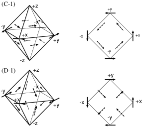
Figure 3: Schematic picture of spin structure for (C-1) and (D-1). The right panels in (C-1) and (D-1) show the top views, i.e. the views from the [001]-direction.

The difference in magnetic point groups is also reflected in difference in a possible ME effect. The ME property tensor $\bm{G}$ in the term $G_{ij}H_{i}E_{j}$ in the free energy is easily written down for each magnetic point group birss :

$$\mbox{(C-1)}\left(\begin{array}[]{ccc}0&G_{1}&0\\ -G_{1}&0&0\\ 0&0&0\end{array}\right),\ \mbox{(D-1)}\left(\begin{array}[]{ccc}0&G_{1}&0\\ G_{1}&0&0\\ 0&0&0\end{array}\right),$$

in the original Cartesian coordinates of the cubic lattice. The property tensor $\bm{G}$ is antisymmetric in (C-1), which implies $\bm{M}\bot\bm{E}$ and $\bm{P}\bot\bm{B}$. Thus, measurement of the ME effect with a single crystal of CaB₆ will reveal which of these two cases is realized. Experimentally, there are two types of AF domains, and the sign of the property tensor $\bm{G}$ is reversed when the staggered magnetization is reversed. In measurement of the ME effect, alignment of the domain structure is necessary. It is accomplished by means of a magnetoelectric annealing, in which the sample is cooled under both electric and magnetic fields. Experimentally, CaB₆ is not insulating, though the sample dependence is rather large. Therefore, we cannot apply electric field into the sample; we can neither perform magnetoelectric cooling nor the measurement of magnetoelectric effect. We should then resort to the optical measurements described in the next section.

Domain boundaries between the two AF domains can exhibit interesting properties. As in boundaries between two SC domains with broken time-reversal symmetry su , localized current and magnetic moment are induced near the boundary. In the present case it is interpreted as the ME effect.

It is reported that weak diamagnetism is often observed in CaB₆ morikawa ; young . It can be attributed to orbital motion, as in the Landau diamagnetism. In semimetals like Bi and narrow-gap semiconductors, such diamagnetism appears. In Bi, in particular, it is proposed as orbital diamagnetism fukuyama . Hence, it is no wonder that the small band gap/overlap in CaB₆ originates diamagnetism. In reality, it is easily hidden by the AF or by the ferromagnetism near the surface.

IV.2 Optical Properties

Optical measurements are known as powerful tools in identifying the magnetic properties of the material. In optical measurements, there are wide range of choices for tuning parameters, such as polarization and incident direction of light, providing us with lots of information of the material. One of the most spectacular examples is Cr₂O₃, where the second-harmonic generation (SHG) is utilized to get the image of the antiferromagnetic domains for the first time ffsp . As shown in this example, magnetoelectrics such as Cr₂O₃ generally exhibit novel optical properties. Since our theory predicts that the present material CaB₆ is among the magnetoelectrics, its magnetic symmetry can be checked by various optical experiments. For example, nonreciprocal (NR) optical effects bst ; fuchs ; gr92 occur in the magnetoelectrics, since the ME tensor appears in the formulation of the NR effects gr92 . In other words the ME effect corresponds to a static limit of the optical NR effects. Possible NR effects for all the magnetic point groups of magnetoelectrics are calculated in Ref. gr92, for transmission and in Ref. gr99, for reflection. Let us apply the essential results in these references. Here we note a difference in notation from Ref. gr92, ; gr99, ; for (D-1) $4^{\prime}/{\rm m}^{\prime}{\rm m}^{\prime}{\rm m}$ the $x$ and $y$ axes are rotated by 45 degrees around the $z$-axis from those in Ref. gr92, ; gr99, .

IV.2.1 Optical Nonreciprocal Effects

According to Ref.gr92, , the multipole expansion of electric and magnetic fields gives rise to various tensors, each of which is responsible for various optical effects. To the order of electric quadrupoles and magnetic dipoles, nonvanishing tensors in an $RI$-invariant system such as CaB₆ are the polar i-tensor $\alpha_{\alpha\beta}(\omega)$, the polar c-tensor $a^{\prime}_{\alpha\beta\gamma}(\omega)(=a^{\prime}_{\alpha\gamma\beta}(\omega))$, and the axial c-tensor $G_{\alpha\beta}(\omega)$ in the notation of Ref. gr92, , where $\alpha_{\alpha\beta}(\omega)$ is the polarizability tensor, while $a^{\prime}_{\alpha\beta\gamma}(\omega)$ and $G_{\alpha\beta}(\omega)$ are assigned to the NR optical effects. Note that the static limit $G_{\alpha\beta}(\omega=0)$ is just the ME property tensor $G_{\alpha\beta}$. Magnetic symmetry determines nonvanishing components of these tensors. We can then calculate the refractive index using these tensors. The detailed derivation is developed in Appendix A, and here we present only the results. Let $n=n^{\prime}+{\rm i}n^{\prime\prime}$ denotes the complex refractive index, where the real part $n^{\prime}$ is the refractive index and the imaginary part $n^{\prime\prime}$ is the absorption coefficient. We also define $\bm{\sigma}$ as $\bm{\sigma}=\bm{k}/k$, i.e. a normal vector along the incident direction of light. The refractive index $n$ for light along the $\pm z$-direction $\bm{\sigma}=(0,0,\sigma_{z})=(0,0,\pm 1)$ is obtained for two types of polarization as

$$\mbox{(C-1)}:$$

$$\makebox[14.22636pt]{}\left[\bm{E}\|\hat{x},\bm{E}\|\hat{y}\right]:n=\frac{c}{2}\left(\sigma_{z}\mu_{0}C_{5}+\sqrt{\mu_{0}^{2}C_{5}^{2}+4\mu_{0}\epsilon_{x}}\right),$$

$$\mbox{(D-1)}:\left[\bm{E}\|\hat{x}\right]:\ n=\frac{c}{2}\left(\sigma_{z}\mu_{0}C_{5}+\sqrt{\mu_{0}^{2}C_{5}^{2}+4\mu_{0}\epsilon_{x}}\right),$$

$$\makebox[30.00005pt]{}\left[\bm{E}\|\hat{y}\right]:\ n=\frac{c}{2}\left(-\sigma_{z}\mu_{0}C_{5}+\sqrt{\mu_{0}^{2}C_{5}^{2}+4\mu_{0}\epsilon_{x}}\right),$$

where $C_{5}=2G_{xy}+\omega a^{\prime}_{xxz}$. Note that since $G_{\alpha\beta}$ and $a^{\prime}_{\alpha\beta\gamma}$ are c-tensors, $C_{5}$ changes sign for different AF domains, which are related with each other by the time-reversal. Thus, for a single domain, (C-1) shows a directional birefringence, but there is no anisotropy in polarization, i.e. no birefringence in the usual sense. In (D-1), on the other hand, directional birefringence and usual birefringence both exist. Hence, linearly-polarized light can distinguish between these two cases. In fact we do not even need to fix polarization; unpolarized light is sufficient to distinguish between these two possibilities. Unpolarized light, which is an incoherent superposition of both $x$- and $y$-polarized lights, shows a refractive index of an average of two refractive indices for two types of polarizations

(C-1) $$: n=\frac{c}{2}\left(-\sigma_{z}\mu_{0}C_{5}+\sqrt{\mu_{0}^{2}C_{5}^{2}+4\mu_{0}\epsilon_{x}}\right),$$ (24)

(D-1) $$: n=\frac{c}{2}\sqrt{\mu_{0}^{2}C_{5}^{2}+4\mu_{0}\epsilon_{x}}.$$ (25)

Therefore, only in (C-1) does the system show directional birefringence for unpolarized light along the tetragonal axis. This effect, i.e. directional birefringence for unpolarized lights, is called a magnetochiral effect rikken . This effect is more prominent in the high-frequency region as evidenced in the X-ray measurement of Cr-doped V₂O₃ x .

Experimentally, domain structure is formed, which might obscure the experimental results. If we assume that the sample is a single crystal with perfect cubic structure above the Néel temperature $T_{N}$, there are two sources of domain formation below $T_{N}$. One is (a) the AF domains of opposite staggered moments, while the tetragonal axis are common. The other is (b) the domains due to different direction of tetragonal distortion below $T_{N}$. This domain formation will affect the NR optical effects in the following way. For the (a)-type domains, the parameters $C_{5}$ has different signs for different AF domains, which smears out the NR effects. Thus, the thin-film sample should have a single domain in the direction of light propagation. On the other hand, for the (b)-type domains, we can investigate the problem by setting the incident direction as $x$ or $y$ direction in the above equations. The result for $\bm{\sigma}=(\sigma_{x},0,0)=(\pm 1,0,0)$ is

$$\left[\bm{E}\|\hat{y}\right]:\ n=\sqrt{\epsilon_{0}^{-1}\epsilon_{x}},$$

$$\left[\bm{E}\|\hat{z}\right]:\ n=\sqrt{\epsilon_{0}^{-1}\epsilon_{x}}\left(1+\frac{\mu_{0}}{\epsilon_{x}}C_{7}\right)^{-\frac{1}{2}},$$

for both (C-1) and (D-1), where we set $C_{7}=-G_{xy}+\frac{1}{2}\omega(a^{\prime}_{zxx}+a^{\prime}_{xxz})$. For the incident direction parallel to the $y$-direction, the result is similar, with $\bm{E}\|\hat{y}$ and $\bm{E}\|\hat{x}$ being interchanged in the above result. These imply that for $\bm{\sigma}\|\hat{x}$ and $\bm{\sigma}\|\hat{y}$ the NR optical effects do not take place. Thus only the light traveling parallel to the $z$-axis undergoes the NR optical effect; hence the (b)-type domains will not hinder the identification of ground states by the NR effect, although it is reduced by the factor of 3.

In reflection, on the other hand, within the method in Ref. gr99, , the reflection matrix $R$ for light propagating along the $z$-axis defined by

$$(E_{{\rm r}})_{j}=R_{jk}(E_{{\rm i}})_{k}$$ (26)

is proportional to identity for both (C-1) and (D-1), where $E_{\text{i}}$ and $E_{\text{r}}$ are the electric fields for incident and reflected lights, respectively. This implies that there is no optical NR effect in reflection normal to the $xy$-plane. Nevertheless, since this effect is not prohibited by symmetry, this NR effect in reflection can emerge in higher order than in Ref. gr99, . We note that in reflection experiments, the surface inevitably affects the spectrum dp . Thus, even if the NR effect in reflection are observed, it might be difficult to separate the result into the surface and bulk contributions, as it is controversial in Cr₂O₃.

IV.2.2 Second Harmonic Generation

Second harmonic generation (SHG) is recently emerging as a new and powerful tool for determination of magnetic symmetry of the material. This effect appears both in transmission and in reflection. For separating bulk contribution from surface one, transmission measurement is preferable. At the surface the inversion symmetry is always broken, and the SHG always emerges. It is difficult to separate bulk and surface contributions in reflection measurement.

This SHG can arise from various multipole contributions, among which an electric-dipole one is the most dominant in general. This arises from the third nonlinear dielectric constant $\chi_{ijk}^{e}$ defined as

$$P_{i}(2\omega)=\chi_{ijk}^{e}(2\omega;\omega,\omega)E_{j}(\omega)E_{k}(\omega)$$ (27)

and is nonzero only if the spatial inversion $I$ is broken. Thus this electric-dipole SHG appears either at a bulk with broken inversion symmetry or at surfaces. Depending on magnetic symmetry of the compound, the SHG emerges in a different way by varying the incident direction or polarization of light, and by changing which polarization is measured. Therefore, by measuring the SHG intensity for various experimental settings, magnetic symmetry of the material can be almost uniquely determined, as the recent examples of YMnO₃ and Cr₂O₃ show ffkp ; spin-flop ; YMO98 ; YMO99 .

CaB₆ is not an exception. Two candidates for its magnetic symmetry, (C-1) $4/\text{m}^{\prime}\text{mm}$ and (D-1) $4^{\prime}/\text{m}^{\prime}\text{m}^{\prime}\text{m}$, can be distinguished by the SHG, as we shall see below. Because CaB₆ breaks inversion symmetry according to our prediction, this electric-dipole SHG is nonvanishing in the bulk. The third nonlinear dielectric constant $\chi_{ijk}^{e}$ is decomposed into two parts $\chi_{ijk}^{e}=\chi_{ijk}^{e(i)}+\chi_{ijk}^{e(c)}$, where $\chi_{ijk}^{e(i)}$ and $\chi_{ijk}^{e(c)}$ are $i$-tensors (invariant under time-reversal $R$) and $c$-tensors (change sign under $R$), respectively. In CaB₆, the $RI$-invariance yields $\chi_{ijk}^{e(i)}=0$. The magnetic point-group symmetry of the system determines which components of the tensor $\chi_{ijk}^{e(c)}$ are vanishing. We can calculate the intensity of the SHG for any choice of incident direction and polarization. Among the various choices the simplest one is the light propagating along the $z$-axis, i.e. the $c$-axis in the tetragonal crystal. As shown in Appendix B, however, the SHG cannot arise in this setting. Thus, the sample must be tilted to observe the SHG, as in YMnO₃ YMO98 ; YMO99 . The simplest choice of tilting of the sample is around the [100] axis. It is, however, not convenient for the identification of magnetic symmetry for CaB₆ ; the difference between the two possibilities (C-1) and (D-1) is not conspicuous with this choice. Instead, we shall tilt the crystal around the [110] axis while the incident direction is fixed as $\bm{k}\|\hat{z}$. Let $\phi$ denote the tilting angle phi , which is fixed throughout the whole measurement. The details of the calculation is presented in Appendix B. Among various choices of polarization of the incoming light $\bm{E}(\omega)$ and that measured by the detector, we find the following; when we wish to see the difference between the two cases (C-1) (D-1), the best way is to measure the SHG intensity for the polarization perpendicular to that of the incoming light $\bm{E}(\omega)$. Let $P(2\omega)_{\bot}$ denote the component of $\bm{P}(2\omega)$ perpendicular to the incident polarization. Then we get

$$\mbox{(C-1)}:P_{\bot}=E_{x}\frac{\epsilon_{0}\sin\phi}{\sqrt{E_{x}^{2}+E_{y}^{2}}}\left(2\chi_{xxz}^{e(c)}E_{y}^{2}\sin^{2}\phi\right.$$

$$\makebox[22.76219pt]{}\left.-\chi_{zxx}^{e(c)}(E_{x}^{2}+E_{y}^{2}\cos^{2}\phi)-\chi_{zzz}^{e(c)}E_{y}^{2}\sin^{2}\phi\right),$$ (28)

$$\mbox{(D-1)}:P_{\bot}=E_{y}\frac{\epsilon_{0}\sin\phi}{\sqrt{E_{x}^{2}+E_{y}^{2}}}\left(2\chi_{xxz}^{e(c)}(E_{y}^{2}-E_{x}^{2})\cos\phi\right.$$

$$\makebox[22.76219pt]{}\left.-2\chi_{zxx}^{e(c)}E_{x}^{2}\cos\phi-\chi_{zzz}^{e(c)}E_{x}E_{y}\sin^{2}\phi\right).$$ (29)

The SHG intensity is proportional to $P_{\bot}^{2}$. Thus we propose the following experiment for distinguishing (C-1) and (D-1). As the polarization of the incoming light is rotated, and polarization measured by the detector is rotated accordingly as is perpendicular to $\bm{E}(\omega)$, we should measure the change of the SHG intensity. In (C-1) the SHG intensity vanishes when $E_{x}=0$ and in (D-1) it vanishes when $E_{y}=0$. Thus, in this measurement we can distinguish between these two. This SHG is observed only below $T_{N}$, which will be an evidence of magnetic ordering in the parent compound CaB₆.

Let us consider an effect of domain formation on the SHG. For the (a)-type domains, $\chi$’s change sign for different domains; this does not, however, affect the SHG intensity, which is proportional to $P_{\bot}^{2}$. Thus the type (a) domains will do no harm. On the other hand, the (b)-type domains will kill the difference between (C-1) and (D-1), as explained below. If the tetragonal distortion is along the $x$- or $y$-axis instead of the $z$-axis, we can calculate in the similar way as above. The resulting form of $P_{\bot}$ is so complicated that we do not reproduce here. Unlike (28) (29), $P_{\bot}$ cannot be factorized, i.e. there is no node when the incident polarization is rotated. If this type of domains are mixed along the direction of light propagation, the SHG intensity does not have no node, and we can no longer distinguish between (C-1) and (D-1). Therefore, we should make sure that this (b)-type domains are not mixed. This can be verified by an untilted $(\phi=0)$ setting. If there is only a single domain, we can use (28)(29) and the SHG intensity vanishes when $\phi=0$. An existence of the (b)-type domains will give nonzero intensity. To avoid the mixture of these (b)-type domains, a choice of substrate material will be important. It is expected that a good choice of substrate material for thin-film fabrication will uniquely set the direction of tetragonal distortion to be perpendicular to the thin-film.

In cases such as Cr₂O₃, contribution from magnetic dipole cannot be neglected. Let us, therefore, consider this contribution for CaB₆. This comes from the SH magnetic-dipole tensor $\chi_{ijk}^{m}$ defined by

$$M_{i}(2\omega)=\frac{\epsilon_{0}c}{n}\chi_{ijk}^{m}(2\omega;\omega,\omega)E_{j}(\omega)E_{k}(\omega).$$ (30)

Since this is an axial tensor, the $RI$-symmetry in CaB₆ allows only the $i$-tensor component $\chi_{ijk}^{m(i)}$. Hence it persists both below and above the Néel temperature. Nevertheless, we show in Appendix C that when we measure the polarization of the SHG perpendicular to $\bm{E}(\omega)$, this magnetic-dipole contribution never appears. This is another merit of our experimental setting.

The AF domain topography by the SHG ffsp ; spin-flop ; YMO00 is also possible in this material. Domain topography utilizes an interference between the $c$-tensor $\chi^{(c)}$ and the $i$-tensor component $\chi^{(i)}$. Thus we should have the SHG from both contributions at the same time for domain topography. At least the detected polarization should not be perpendicular to the incident polarization. To obtain better contrast for two types of domains, the polarization of the incident light and that of detected light should be tuned YMO99 .

V Discussion and Conclusion

Now we discuss the relevance of our results to various experiments on CaB₆ and Ca_1-xLa_xB₆. We believe many of the novel magnetic properties can be interpreted as the ME effect. The ferromagnetism in the thin-film CaB₆ is interpreted as caused by an electric field between vacuum and the substrate. For the powder sample experiment and the La-doping experiment, the explanation is more delicate. We believe that the carriers by La-doping is trapped by impurities/defects and create local electric fields. Therefore in these cases, an internal electric field and/or a gradient of a strain has a random direction, and hence the magnetic moment is induced locally due to this mechanism. Without an external magnetic field, they almost cancel with each other, giving zero or quite small uniform magnetization, which appears to contradict with the experiments. In fact it is consistent with experiments. The compound shows hysteresis, which is thought as an experimental evidence for “ferromagnetism”. This is quite opposite to our intuition. The present compound is AF, which usually does not show hysteresis behavior in the $M$-$H$ curve; it is a novel feature of doped AF magnetoelectrics. Hysteresis implies that the free energy has a double minimum as a function of magnetization. In a first sight it is unique to ferromagnets; we propose that this is also the case for Ca_1-xLa_xB₆, which we claim is not ferromagnet in the bulk. In this material, there is a local electric field induced by doped impurities. When we vary the magnetic field, the two AF domains will switch to each other to minimize the free energy. As we explain below, Gibbs free energy acquires two minima as a function of $M$ in the presence of local electric field, which causes hysteresis. Considering that the ME tensor $G$ is proportional to the exciton order parameters $\text{Im}\eta$, we can write the Gibbs free energy $F$ as

$$F=-C(\text{Im}\eta)PM+\frac{1}{2\chi}M^{2}+\frac{1}{2\alpha}P^{2}-A(\text{Im}\eta)^{2}$$

$$\makebox[28.45274pt]{}+B(\text{Im}\eta)^{4}-DP\text{Re}\eta,$$ (31)

where $A,B,C,\chi,\alpha$ are positive constants and $D$ is a constant. Here, for simplicity, we omitted subscripts for $P$, $M$, $\eta$ without loss of generality. By minimizing $F$ in terms of $\text{Im}\eta$, we obtain $\text{Im}\eta\sim\text{sgn}(PM)\sqrt{A/2B}$, provided $C$ is small. When we substitute it into $F$, we get

$$F\sim-C\sqrt{\frac{A}{2B}}|P||M|+\frac{1}{2\chi}M^{2}+\frac{1}{2\alpha}P^{2}-DP\text{Re}\eta.$$ (32)

Near the doped impurities, the polarization $P$ is induced by a local electric field. In this case, $P$, $M$, and $\eta$ has spatial dependence and should be written as $P(\bm{x})$, $M(\bm{x})$, $\eta(\bm{x})$. Although the sign of $P(\bm{x})$ changes spatially, one can basically regard $|P(\bm{x})|$ as a constant. In the presence of $P$, this Gibbs free energy has two minima as a function of $M$, implying hysteresis. Note that this is not a genuine ferromagnet; a uniform $M(\bm{x})$ does not emerge in the absence of an external magnetic field, because the uniform $M(\bm{x})$ costs an elastic energy $(\nabla\text{Im}\eta(\bm{x}))^{2}$. On the other hand, If there is no impuritiy, i.e. $P=0$, $F$ does not have double-minimum structure, and no hysteresis results. Hence, hysteresis in Ca_1-xLa_xB₆ can result from the ME effect together with the local electric field near doped impurities.

Because Ca_1-xLa_xB₆ is not insulating, the electric field is screened. The Thomas-Fermi screening length is estimated as

$$\frac{\sqrt{a_{0}\epsilon}}{2}\left(\frac{\pi}{3n_{0}}\right)^{\frac{1}{6}}\sim 10\text{\AA},$$ (33)

where $a_{0}$ is the Bohr radius, and we used the values $\epsilon\sim 6$ for the dielectric constant gavilano and $n_{0}\sim(1\mbox{-}4)\times 10^{24}{\rm m}^{-3}$ for a density of electrons gianno . The appearance of magnetic moments via the ME effect is therefore localized within this screening length of the impurities or surfaces.

Other peculiarities of Ca_1-xLa_xB₆ can also be explained as well. The high Curie temperature $(\sim 600{\rm K})$ is nothing but a Néel temerature of the parent compound CaB₆, and is not contradictory with a tiny magnetic moment. A rather narrow range ($x\lesssim 0.01$) of La-doping allowing ferromagnetism is attributed to fragility of excitonic order by a small amount of impurities sk ; z . Moreover, our scenario is also consistent with the experimental results that deficiency in Ca sites morikawa or doping of divalent elements like Ba young or Sr ott induces ferromagnetism. It is also confirmed numerically by a supercell approach that imperfections and surfaces can induce local moments md . It is hard to explain them within the spin-doping scenario zra . Furthermore, strangely enough, it is experimentally hard to find a correlation between magnetism and electrical resistivity, as seen in magnetizaion morikawa and in nuclear magnetic resonance gavilano . This novelty can be considered as natural consequence of our scenario; electrical resistivity should be mainly due to doped carriers by La, while the magnetization is due to local lattice distortion and/or electric field.

The ESR experiments by Kunii kunii also support the above scenario. The ESR data show that in a disk-shaped Ca_1-xLa_xB₆ ($x=0.005$), the magnetic moment only exists within the surface layer. Furthermore, the moment $\bm{M}$ does not orient in the direction of $\bm{H}$, i.e. it feels strong magnetic anisotropy to keep the moment within the disk plane. This might be due to the long-range dipolar energy, and not due to the above scenario. Nevertheless, it is unlikely that the long-range dipolar energy causes such a strong anisotropy. This point requires further experimental and theoretical investigation. Let us, for the moment, assume that this strong anisotropy is mainly caused by the exciton condensation and the ME mechanism. Since this electric field should be perpendicular to the plane, the strong easy-plane anisotropy parallel to the surface implies that $\bm{M}\bot\bm{E}$. Therefore, among the four cases, (C-1) or (C-2) are compatible, i.e. the excitons corresponding to $\bm{\eta}(\Gamma_{15},1)$ and $\bm{\eta}(\Gamma_{15},2)$ simultaneously condense. Considering the Raman scattering data, we conclude that (C-1) is the only possibility compatible with the experiments.

We briefly mention the relationship between our theory and the theories in Refs. zra, ; bv, . In the absence of doping, our theory is consistent with Refs. zra, ; bv, . The difference lies in the mechanism of ferromagnetism in doping. We proposed that defects, impurities or surfaces induce ferromagnetism. This is different from Refs. zra, ; bv, , in which ferromagnetism is due to spin alignment of doped carriers. We should note that these two mechanisms can coexist. We can distinguish these two contributions for ferromagnetism by systematically changing the valence of doped impurities. In doping with divalent doping, no carriers are doped, and the moment is due to our scenario. Difference between trivalent- and divalent-doping corresponds to the scenarios in Refs. zra, ; bv, . Our theory is treating the dilute doping limit. We also note that because our theory is based on the GL theory, it is treating an instability in slight doping. Thus our conclusions do not hinder an appearance of rich phase diagrams, as presented, for example, in Ref. zra, ; bv, ; b, ; vb, ; bbm, .

We mention here a role of the spin-orbit coupling. In the absence of the spin-orbit coupling, the GL free energy $\Phi^{(2)}$ for the imaginary parts of the order parameters is written as

$$\Phi^{(2)}=\lambda_{+}^{{\rm Im}}\sum_{i}({\rm Im}\ \eta_{i}(\Gamma_{15},+))^{2}$$

$$\makebox[1.42262pt]{}+\lambda_{-}^{{\rm Im}}\sum_{i}({\rm Im}\ \eta_{i}(\Gamma_{15},-))^{2}+\lambda_{\Gamma_{25}}^{{\rm Im}}\sum_{j}({\rm Im}\ \eta_{j}(\Gamma_{25}))^{2},$$

from (71) in Appendix D. As $\lambda_{+}^{{\rm Im}}>\lambda_{-}^{{\rm Im}}=\lambda_{\Gamma_{25}}^{{\rm Im}}$ from the aforementioned microscopic calculation, the condensation of excitons in $\Gamma_{15}$ and those in $\Gamma_{25}$ occur simultaneously. Furthermore, inspection of $\Phi^{(4)}$ in the absence of the spin-orbit coupling shows that the quartic-order terms in the GL free energy do not lift this degeneracy. Sixth-order terms will lift it, and a resulting state will belong to either 4/${\rm m}^{\prime}{\rm m}^{\prime}{\rm m}^{\prime}$ or $4^{\prime}/{\rm m}^{\prime}{\rm m}^{\prime}{\rm m}$. The details are presented in Appendix D. Both of them still lead to the ME effect in the absence of the spin-orbit coupling; this ME effect must be generated from an orbital motion. Thus, the AF state in CaB₆ has an orbital nature as well as a spin nature. With spin-orbit interaction, these two are inseparably mixed together.

Recently, similar novel ferromagnets such as CaB₂C₂ akimitsu and rhombohedral C₆₀ makarova have been discovered. They share several properties with CaB₆, i.e. high Curie temperature, smallness of the moment and lack of partially-filled $d$- or $f$-bands. They might be explained by the similar scenario as in CaB₆, and indeed one of the authors explained the novel ferromagnetism in CaB₂C₂ within the scenario of exciton condensation murakami .

In conclusion, we have studied the symmetry properties of the excitonic state in the parent compound CaB₆, and found that the triplet excitonic state with broken time-reversal and inversion symmetries offers a natural explanation, in terms of the ME effect, for the novel ferromagnetism emerging in La-doping or thin-film fabrication. This scenario can be tested experimentally by measurements of the ME effect and the optical non-reciprocal effect in single crystal of the parent compound CaB₆.

Appendix A Derivation of the refractive index – optical nonreciprocal effects –

Nonvanishing components for each tensor of the optical nonreciprocal (NR) effects are determined from each magnetic point group as birss

(C-1) $$: \alpha_{xx}=\alpha_{yy},\ \ \ \alpha_{zz},$$

$$G_{xy}=-G_{yx},$$

$$a^{\prime}_{xxz}=a^{\prime}_{xzx}=a^{\prime}_{yyz}=a^{\prime}_{yzy},$$

$$a^{\prime}_{zxx}=a^{\prime}_{zyy},\ \ \ a^{\prime}_{zzz},$$

(D-1) $$: \alpha_{xx}=\alpha_{yy},\ \ \ \alpha_{zz},$$

$$G_{xy}=G_{yx},$$

$$a^{\prime}_{xxz}=a^{\prime}_{xzx}=-a^{\prime}_{yyz}=-a^{\prime}_{yzy},$$

$$a^{\prime}_{zxx}=-a^{\prime}_{zyy}.$$

In calculating the optical properties in transmission or in reflection, the tensor $\tilde{A}_{\alpha\beta\gamma}$ defined as

$$\tilde{A}_{\alpha\beta\gamma}=\tilde{A}_{\beta\alpha\gamma}$$

$$\ \ =-\epsilon_{\beta\gamma\delta}G_{\alpha\delta}-\epsilon_{\alpha\gamma\delta}G_{\beta\delta}+\frac{1}{2}\omega(a^{\prime}_{\alpha\beta\gamma}+a^{\prime}_{\beta\alpha\gamma})$$ (34)

plays a central role gr92 . Its nonvanishing components for each magnetic group are summarized in Table 2 of Ref. gr92, . They are

(C-1) $$: \tilde{A}_{zxx}=\tilde{A}_{xzx}=\tilde{A}_{zyy}=\tilde{A}_{yzy}$$

$$\makebox[28.45274pt]{}=-G_{xy}+\frac{1}{2}\omega(a^{\prime}_{zxx}+a^{\prime}_{xxz}),$$

$$\tilde{A}_{xxz}=\tilde{A}_{yyz}=2G_{xy}+\omega a^{\prime}_{xxz},$$

$$\tilde{A}_{zzz}=\omega a^{\prime}_{zzz},$$

(D-1) $$: \tilde{A}_{zxx}=\tilde{A}_{xzx}=-\tilde{A}_{zyy}=-\tilde{A}_{yzy}$$

$$\makebox[28.45274pt]{}=-G_{xy}+\frac{1}{2}\omega(a^{\prime}_{zxx}+a^{\prime}_{xxz}),$$

$$\tilde{A}_{xxz}=-\tilde{A}_{yyz}=2G_{xy}+\omega a^{\prime}_{xxz},$$

The refractive index $n$ for each polarization is obtained as a solution of the following equation.

$$\left[n^{2}(\sigma_{\alpha}\sigma_{\beta}-\delta_{\alpha\beta})+\delta_{\alpha\beta}+\epsilon_{0}^{-1}\alpha_{\alpha\beta}+c\mu_{0}n\sigma_{\gamma}\tilde{A}_{\alpha\beta\gamma}\right]$$

$$\cdot E_{\beta}=0.$$ (35)

For incident direction along the $\pm z$-direction $\bm{\sigma}=\bm{k}/k=(0,0,\sigma_{z})=(0,0,\pm 1)$, an equation determining the refractive index $n$ is

$$\mbox{(C-1)}:\left(\begin{array}[]{ccc}-n^{2}+\epsilon_{0}^{-1}\epsilon_{x}+c\mu_{0}nC_{5}\sigma_{z}&&\\ &-n^{2}+\epsilon_{0}^{-1}\epsilon_{x}+c\mu_{0}nC_{5}\sigma_{z}&\\ &&\epsilon_{0}^{-1}\epsilon_{z}+c\mu_{0}nC_{6}\sigma_{z}\end{array}\right)\left(\begin{array}[]{c}E_{x}\\ E_{y}\\ E_{z}\end{array}\right)=0,$$ (42)

$$\mbox{(D-1)}:\left(\begin{array}[]{ccc}-n^{2}+\epsilon_{0}^{-1}\epsilon_{x}+c\mu_{0}nC_{5}\sigma_{z}&&\\ &-n^{2}+\epsilon_{0}^{-1}\epsilon_{x}-c\mu_{0}nC_{5}\sigma_{z}&\\ &&\epsilon_{0}^{-1}\epsilon_{z}\end{array}\right)\left(\begin{array}[]{c}E_{x}\\ E_{y}\\ E_{z}\end{array}\right)=0,$$ (49)

where $\epsilon_{x}=\epsilon_{0}+\alpha_{xx}=\epsilon_{0}+\alpha_{yy}$, $\epsilon_{z}=\epsilon_{0}+\alpha_{zz}$ $C_{5}=2G_{xy}+\omega a^{\prime}_{xxz}$, and $C_{6}=\omega a^{\prime}_{zzz}$. Thus for both cases the refractive index $n$ is given by

$$\mbox{(C-1)}:\left[\bm{E}\|\hat{x},\ \bm{E}\|\hat{y}\right]:n=\frac{c}{2}\left(\sigma_{z}\mu_{0}C_{5}+\sqrt{\mu_{0}^{2}C_{5}^{2}+4\mu_{0}\epsilon_{x}}\right),$$

$$\mbox{(D-1)}:\left[\bm{E}\|\hat{x}\right]:\ n=\frac{c}{2}\left(\sigma_{z}\mu_{0}C_{5}+\sqrt{\mu_{0}^{2}C_{5}^{2}+4\mu_{0}\epsilon_{x}}\right),$$

$$\makebox[30.00005pt]{}\left[\bm{E}\|\hat{y}\right]:\ n=\frac{c}{2}\left(-\sigma_{z}\mu_{0}C_{5}+\sqrt{\mu_{0}^{2}C_{5}^{2}+4\mu_{0}\epsilon_{x}}\right),$$

for $\bm{\sigma}=(0,0,\pm 1)$.

In order to consider an effect of domain formation of the (b)-type, i.e. domains with different directions of distortion, let us study the light propagating along the $x$-direction in the similar way as above. An equation for $\bm{\sigma}=(\sigma_{x},0,0)=(\pm 1,0,0)$ is

$$\left(\begin{array}[]{ccc}\epsilon_{0}^{-1}\epsilon_{x}&&c\mu_{0}nC_{7}\sigma_{x}\\ &-n^{2}+\epsilon_{0}^{-1}\epsilon_{x}&\\ c\mu_{0}nC_{7}\sigma_{x}&&-n^{2}+\epsilon_{0}^{-1}\epsilon_{z}\end{array}\right)\left(\begin{array}[]{c}E_{x}\\ E_{y}\\ E_{z}\end{array}\right)=0,$$

for both (C-1) and (D-1), where we set $C_{7}=-G_{xy}+\frac{1}{2}\omega(a^{\prime}_{zxx}+a^{\prime}_{xxz})$. Thus the refractive index is

$$\left[\bm{E}\|\hat{y}\right]:\ n=\sqrt{\epsilon_{0}^{-1}\epsilon_{x}},$$

$$\left[\bm{E}\|\hat{z}\right]:\ n=\sqrt{\epsilon_{0}^{-1}\epsilon_{z}}\left(1+\frac{\mu_{0}}{\epsilon_{x}}C_{7}\right)^{-\frac{1}{2}},$$

for $\bm{\sigma}=(\pm 1,0,0)$. The latter one with $\bm{E}\|\hat{z}$ contains a longitudinal component of $\bm{E}$, i.e. parallel to $\hat{x}$. It is called an S-wave (skew wave) in Ref. gr92, , and can only propagate only inside the sample. For $\bm{\sigma}=(0,\pm 1,0)$, we get

$$\left[\bm{E}\|\hat{x}\right]:\ n=\sqrt{\epsilon_{0}^{-1}\epsilon_{x}},$$

$$\left[\bm{E}\|\hat{z}\right]:\ n=\sqrt{\epsilon_{0}^{-1}\epsilon_{z}}\left(1+\frac{\mu_{0}}{\epsilon_{x}}C_{8}\right)^{-\frac{1}{2}},$$

These imply that for $\bm{\sigma}\|\hat{x}$ and $\bm{\sigma}\|\hat{y}$ the NR optical effects do not take place.

Appendix B Calculation of the SHG intensity to distinguish (C-1) and (D-1)

The nonvanishing components of the nonlinear electric-dipole tensor $\chi_{ijk}^{e(c)}$ (polar c-tensor) are given as birss

(C-1) $$: \chi_{zzz}^{e(c)},\ \ \ \chi_{zxx}^{e(c)}=\chi_{zyy}^{e(c)},$$

$$\chi_{xzx}^{e(c)}=\chi_{xxz}^{e(c)}=\chi_{yzy}^{e(c)}=\chi_{yyz}^{e(c)},$$

(D-1) $$: \chi_{zzz}^{e(c)},\ \ \ \chi_{zxx}^{e(c)}=-\chi_{zyy}^{e(c)},$$

$$\chi_{xzx}^{e(c)}=\chi_{xxz}^{e(c)}=-\chi_{yzy}^{e(c)}=-\chi_{yyz}^{e(c)}.$$

By using them, we can derive the equations for the SHG, as in Cr₂O₃ffkp . The nonlinear polarization $\bm{P}(2\omega)$ induced by $\chi_{ijk}^{e}$ is

$$\mbox{(C-1)}:\bm{P}(2\omega)=\epsilon_{0}\left(\begin{array}[]{c}2\chi_{xxz}^{e(c)}E_{x}E_{z}\\ 2\chi_{xxz}^{e(c)}E_{y}E_{z}\\ \chi_{zxx}^{e(c)}(E_{x}^{2}+E_{y}^{2})+\chi_{zzz}^{e(c)}E_{z}^{2}\end{array}\right)$$ (53)

$$\mbox{(D-1)}:\bm{P}(2\omega)=\epsilon_{0}\left(\begin{array}[]{c}2\chi_{xxz}^{e(c)}E_{x}E_{z}\\ -2\chi_{xxz}^{e(c)}E_{y}E_{z}\\ \chi_{zxx}^{e(c)}(E_{x}^{2}-E_{y}^{2})+\chi_{zzz}^{e(c)}E_{z}^{2}\end{array}\right)$$ (57)

These contribute to the source term $\bm{S}^{e}$ for the SHG shen as

$$\bm{S}^{e}=\mu_{0}\frac{\partial^{2}\bm{P}(2\omega)}{\partial t^{2}}=-4\omega^{2}\mu_{0}\bm{P}(2\omega).$$

Therefore, light propagating along the $z$-axis, i.e. the $c$-axis in the tetragonal crystal, $\bm{S}$ is along the $z$-axis and the SHG cannot be generated. Thus, the incident direction must be tilted to observe the SHG, as in YMnO₃ YMO98 ; YMO99 . For practical calculations, it is more convenient to tilt the crystal while fixing the light propagation along the $z$-axis. This kind of treatment is also adopted in Ref. YMO99, . The simplest choice of tilting of the sample is around the [100] axis, but this choice does not manifest clearly the difference between (C-1) and (D-1). Instead, we shall tilt the crystal around the [110] axis while the incident direction is fixed as $\bm{k}\|\hat{z}$. We fix the tilting angle $\phi$, and we fix its value throughout the whole measurement. The calculation is similar to the one for YMnO₃ in Ref. YMO99, . The new coordinate system ($A^{\prime}_{x},A^{\prime}_{y},A^{\prime}_{z}$) fixed to the crystal is related to the original one ($A_{x},A_{y},A_{z}$) as follows;

$$\left(\begin{array}[]{c}A^{\prime}_{x}\\ A^{\prime}_{y}\\ A^{\prime}_{z}\end{array}\right)=\left(\begin{array}[]{ccc}\frac{1}{\sqrt{2}}&\frac{1}{\sqrt{2}}&\\ -\frac{1}{\sqrt{2}}&\frac{1}{\sqrt{2}}&\\ &&1\\ \end{array}\right)\left(\begin{array}[]{ccc}1&&\\ &\cos\phi&\sin\phi\\ &-\sin\phi&\cos\phi\end{array}\right)\left(\begin{array}[]{c}A_{x}\\ A_{y}\\ A_{z}\end{array}\right).$$ (58)

First, the polarization $\bm{E}(\omega)=(E_{x},E_{y},0)$ is transformed to the new coordinate. Then (53) (57) are applied to get the nonlinear polarization $\bm{P}(2\omega)$, and transform it back to the original coordinate ($A_{x},A_{y},A_{z}$). The resulting form for the nonlinear polarization is

$$\mbox{(C-1)}:\bm{P}(2\omega)=\epsilon_{0}\left(\begin{array}[]{c}-2\chi_{xxz}^{e(c)}E_{x}E_{y}\sin\phi\\ -2\chi_{xxz}^{e(c)}E_{y}^{2}\cos^{2}\phi\sin\phi-\chi_{zxx}^{e(c)}(E_{x}^{2}+E_{y}^{2}\cos^{2}\phi)\sin\phi-\chi_{zzz}^{e(c)}E_{y}^{2}\sin^{3}\phi\\ -2\chi_{xxz}^{e(c)}E_{y}^{2}\cos\phi\sin^{2}\phi+\chi_{zxx}^{e(c)}(E_{x}^{2}+E_{y}^{2}\cos^{2}\phi)\cos\phi+\chi_{zzz}^{e(c)}E_{y}^{2}\cos\phi\sin^{2}\phi\\ \end{array}\right),$$ (62)

$$\mbox{(D-1)}:\bm{P}(2\omega)=\epsilon_{0}\left(\begin{array}[]{c}-2\chi_{xxz}^{e(c)}E_{y}^{2}\cos\phi\sin\phi\\ -2(\chi_{xxz}^{e(c)}+\chi_{zxx}^{e(c)})E_{x}E_{y}\cos\phi\sin\phi-\chi_{zzz}^{e(c)}E_{y}^{2}\sin^{3}\phi\\ -2\chi_{xxz}^{e(c)}E_{x}E_{y}\sin^{2}\phi+2\chi_{zxx}^{e(c)}E_{x}E_{y}\cos^{2}\phi+\chi_{zzz}^{e(c)}E_{y}^{2}\sin^{2}\phi\cos\phi\end{array}\right).$$ (66)

In order to see the difference between (C-1) and (D-1), we find that the best way is to measure the SHG intensity for the polarization perpendicular to that of the incoming light $\bm{E}(\omega)$. The projection of $\bm{P}(2\omega)$ onto the direction perpendicular to both $\bm{E}(\omega)$ and $z$-axis is just $P(2\omega)_{\bot}=\bm{P}(2\omega)\cdot\bm{n}_{\bot}$, where $\bm{n}_{\bot}=E_{0}^{-1}(-E_{y},\ E_{x},\ 0),\ E_{0}=\sqrt{E_{x}^{2}+E_{y}^{2}}$. Thus

(C-1) $$: P_{\bot}=\frac{\epsilon_{0}}{\sqrt{E_{x}^{2}+E_{y}^{2}}}E_{x}\sin\phi\left(2\chi_{xxz}^{e(c)}E_{y}^{2}\sin^{2}\phi\right.$$ (67)

$$\makebox[10.00002pt]{}\left.-\chi_{zxx}^{e(c)}(E_{x}^{2}+E_{y}^{2}\cos^{2}\phi)-\chi_{zzz}^{e(c)}E_{y}^{2}\sin^{2}\phi\right),$$

(D-1) $$: P_{\bot}=\frac{\epsilon_{0}}{\sqrt{E_{x}^{2}+E_{y}^{2}}}E_{y}\sin\phi\left(2\chi_{xxz}^{e(c)}(E_{y}^{2}-E_{x}^{2})\cos\phi\right.$$ (68)

$$\makebox[10.00002pt]{}\left.-2\chi_{zxx}^{e(c)}E_{x}^{2}\cos\phi-\chi_{zzz}^{e(c)}E_{x}E_{y}\sin^{2}\phi\right).$$

which are identical with (28)(29). Note that (67) is proportional to $E_{x}$, while (68) is proportional to $E_{y}$; this enables an identification of the true ground state.

Appendix C Magnetic dipole contribution to the SHG

Its nonvanishing components are given as

(C-1)(D-1) $$: \chi_{xyz}^{m(i)}=\chi_{xzy}^{m(i)}=-\chi_{yxz}^{m(i)}=-\chi_{yzx}^{m(i)},$$

$$\chi_{zxy}^{m(i)}=-\chi_{zyx}^{m(i)}.$$

By using them, we can derive the equations for the SHG, as in Cr₂O₃ffkp . The nonlinear magnetization $\bm{M}(2\omega)$ induced by $\chi_{ijk}^{m}$ is

$$\bm{M}(2\omega)=\frac{2\epsilon_{0}c}{n}\chi_{xyz}^{m(i)}E_{y}\sin\phi\left(\begin{array}[]{c}-E_{y}\cos\phi\\ E_{x}\cos\phi\\ E_{x}\sin\phi\end{array}\right)$$

These contribute to the source term $\bm{S}^{m}$ for the SHG shen as

$$\bm{S}^{m} = \mu_{0}\nabla\times\frac{\partial\bm{M}(2\omega)}{\partial t}$$

$$= -\frac{8\omega^{2}}{c^{2}}\chi_{xyz}^{m(i)}E_{y}\sin\phi\cos\phi\left(\begin{array}[]{c}E_{x}\\ E_{y}\\ 0\end{array}\right)$$

$$= -\frac{8\omega^{2}}{c^{2}}\chi_{xyz}^{m(i)}E_{y}\sin\phi\cos\phi\bm{E}.$$

Therefore, this $\bm{S}^{m}$ is parallel to the incident polarization $\bm{E}(\omega)$. Thus, when we measure the polarization of the SHG perpendicular to $\bm{E}(\omega)$, this magnetic-dipole contribution never appears.

Appendix D Limit of Zero Spin-Orbit Coupling

In the absence of the spin-orbit coupling, the GL free energy should be invariant under the spin rotation; by lengthy calculations this leads to relations

$$A_{2}+A_{4}=2A_{1},\ \ A_{2}-A_{4}=A_{3}/\sqrt{2},$$

$$B_{2}+B_{4}=2B_{1},\ \ B_{2}-B_{4}=B_{3}/\sqrt{2}.$$ (70)

When we substitute them into $\Phi^{(2)}$ we get

$$\Phi^{(2)}=\lambda_{+}^{{\rm Im}}\sum_{i}({\rm Im}\ \eta_{i}(\Gamma_{15},+))^{2}+\lambda_{-}^{{\rm Im}}\sum_{i}({\rm Im}\ \eta_{i}(\Gamma_{15},-))^{2}$$

$$\makebox[0.56905pt]{}+\lambda_{\Gamma_{25}}^{{\rm Im}}\sum_{j}({\rm Im}\ \eta_{j}(\Gamma_{25}))^{2}$$

$$\makebox[0.56905pt]{ }+\lambda_{+}^{{\rm Re}}\sum_{i}({\rm Re}\ \eta_{i}(\Gamma_{15},+))^{2}+\lambda_{-}^{{\rm Re}}\sum_{i}({\rm Re}\ \eta_{i}(\Gamma_{15},-))^{2}$$

$$\makebox[0.56905pt]{}+\lambda_{\Gamma_{25}}^{{\rm Re}}\sum_{j}({\rm Re}\ \eta_{j}(\Gamma_{25}))^{2}$$ (71)

where $\bm{\eta}(\Gamma_{15},\pm)$ are new basis functions, defined in (11) (12). The coefficients in (71) are

$$\lambda_{+}^{{\rm Im}}=\frac{3B_{2}-B_{4}}{2},\ \ \lambda_{-}^{{\rm Im}}=\lambda_{\Gamma_{25}}^{{\rm Im}}=B_{4},$$ (72)

$$\lambda_{+}^{{\rm Re}}=\frac{3A_{2}-A_{4}}{2},\ \ \lambda_{-}^{{\rm Re}}=\lambda_{\Gamma_{25}}^{{\rm Re}}=A_{4}.$$ (73)

Eqn.(71) is invariant under the cubic group operations in the orbital space. Thus, each term in (71) can be classified into irreducible representation of the ${\rm O}_{{\rm h}}$ in the orbital space, which facilitates subsequent discussions for magnetic properties. Focusing on the imaginary parts of the order parameters, we get the result

$$\Phi^{(2)}=\sum_{i}\left[\lambda_{+}^{{\rm Im}}\eta(\Gamma^{\prime}_{1},i)^{2}+\lambda_{-}^{{\rm Im}}\sum_{l=u,v}(\eta_{l}(\Gamma^{\prime}_{12},i))^{2}\right],$$ (74)

where

$$\eta(\Gamma^{\prime}_{1},i)=\frac{1}{\sqrt{3}}\sum_{a}{\rm Im}\eta_{i}(\bm{Q}_{a}),$$

$$\eta_{u}(\Gamma^{\prime}_{12},i)=\frac{1}{\sqrt{6}}\ {\rm Im}(2\eta_{i}(\bm{Q}_{z})-\eta_{i}(\bm{Q}_{x})-\eta_{i}(\bm{Q}_{y})),$$

$$\eta_{v}(\Gamma^{\prime}_{12},i)=\frac{1}{\sqrt{2}}\ {\rm Im}(\eta_{i}(\bm{Q}_{x})-\eta_{i}(\bm{Q}_{y})),$$

transform according to the $\Gamma^{\prime}_{1}$ and $\Gamma^{\prime}_{12}$ representations of O_h, respectively, under the rotation of the orbital space. As $\lambda_{+}^{{\rm Im}}>\lambda_{-}^{{\rm Im}}$, the condensation of excitons in $\Gamma^{\prime}_{12}$ occur, and we shall focus only on $\Gamma^{\prime}_{12}$ There are two types of degeneracies in (74). One is in the summation over $i$, which reflects the SU(2) symmetry of the spin space. It will never be lifted in the absence of the spin-orbit coupling. The other is in the summation over $l$, i.e. in the direction in the $\eta_{u}$-$\eta_{v}$ plane. This is lifted in the sixth order in $\eta_{l}$. To see this, let us write down higher order terms. They are written conveniently in terms of a complex order parameter $w=\eta_{u}+{\rm i}\eta_{v}$ as

$$\Phi=K_{1}\sum_{i}|w(\Gamma^{\prime}_{12},i)|^{2}+K_{2}\left(\sum_{i}|w(\Gamma^{\prime}_{12},i)|^{2}\right)^{2}$$

$$\makebox[5.0pt]{}+K_{3}\left(\sum_{i}|w(\Gamma^{\prime}_{12},i)|^{2}\right)^{3}+K_{4}{\rm Re}\left(\sum_{i}[w(\Gamma^{\prime}_{12},i)]^{2}\right)^{3},$$

where $K_{j}$ are constants. This is minimized when

1. ${\rm arg}w=\frac{\pi}{3}n$   if  $K_{4}<0$

2. ${\rm arg}w=\frac{\pi}{6}(2n+1)$   if  $K_{4}>0$,

where $n$ is an integer. The order parameters are

(I) $$({\rm Im}\eta_{i}(\bm{Q}_{x}),\ {\rm Im}\eta_{i}(\bm{Q}_{y}),\ {\rm Im}\eta_{i}(\bm{Q}_{z}))=c(1,1,-2),$$ (75)

(II) $$({\rm Im}\eta_{i}(\bm{Q}_{x}),\ {\rm Im}\eta_{i}(\bm{Q}_{y}),\ {\rm Im}\eta_{i}(\bm{Q}_{z}))=c(1,-1,0),$$ (76)

where we write down only one among three equivalent directions for each case. Both (I) and (II) have tetragonal distortion. The magnetic point group for each case is (I) $4^{\prime}/{\rm m}^{\prime}{\rm m}^{\prime}{\rm m}={\rm D}_{4}\times\{E,\ RI\}$ (II) 4/${\rm m}^{\prime}{\rm m}^{\prime}{\rm m}^{\prime}={\rm D}_{2{\rm d}}\times\{E,\ RI\}$. The ME property tensors are easily written down birss ;

$$\mbox{(I)}\left(\begin{array}[]{ccc}G_{1}&0&0\\ 0&G_{1}&0\\ 0&0&G_{3}\end{array}\right),\ \ \mbox{(II)}\left(\begin{array}[]{ccc}G_{1}&0&0\\ 0&-G_{1}&0\\ 0&0&0\end{array}\right),\ \$$ (77)

in the cubic coordinates. Note that the ME effect in the absence of the spin-orbit coupling cannot originate from spins. This shows that the orbital moment exists in this system.

It is helpful to compare the states (C-1)-(D-2) with (I)(II). The forms of the order parameters are given in Eqs.(14) (15) for (C-1) and (D-1), and in Eqs.(75) (76) for (I)(II). Naively one may expect that (C-1)-(D-2) are included in (I) or (II), because (C-1)-(D-2) assumes nonzero spin-orbit coupling, whereas (I)(II) assumes an absence of the spin-orbit coupling. It is, however, not the case, as seen from the different ME tensors in the two cases. The reason is the following. In the presence of the spin-orbit coupling, the degeneracy in the GL free energy $\Phi$ is lifted in the quartic order, resulting in (C-1)-(D-2). In contrast, without the spin-orbit coupling, the degeneracy is lifted in the sixth order, leading to (I)(II). Because of this difference in the lifting of degeneracy, the realized states are different between the cases with and without the spin-orbit coupling.

References

- (1) D. P. Young, D. Hall, M. E. Torelli, Z. Fisk, J. L. Sarrao, J. D. Thompson, H. R. Ott, S. B. Oseroff, R. G. Goodrich, and R. Zysler, Nature 397 412 (1999).
- (2) D. Ceperley, Nature 397 386 (1999).
- (3) M. E. Zhitomirsky, T. M. Rice and V. I. Anisimov, Nature 402 251 (1999).
- (4) L. Balents and C. M. Varma, Phys. Rev. Lett. 84 1264 (2000).
- (5) B. A. Volkov, Yu. V. Kopaev and A. I. Rusinov, Sov. Phys. JETP 41 952 (1976).
- (6) A. Hasegawa and A. Yanase, J. Phys. C12 5431 (1979).
- (7) S. Massida, A. Continenza, T. M. de Pascale and R. Monnier, Z. Phys. B102 83 (1997).
- (8) D. Hall, D. P. Young, Z. Fisk, T. P. Murphy, E. C. Palm, A. Teklu, and R. G. Goodrich, Phys. Rev. B64 233105 (2001).
- (9) B. I. Halperin and T. M. Rice, in Solid State Physics 21 115 (eds. F. Seitz, D. Turnball, and H. Ehrenfest, Academic Press, New York 1968).
- (10) H. J. Tromp, P. van Gelderen, P. J. Kelly, G. Brocks, and P. A. Bobbert, Phys. Rev. Lett. 87, 016401 (2001): in GW, and represents the Green’s function and the screened Coulomb potential, respectively. The self-energy is given by the product of these two.
- (11) J. D. Denlinger, J. A. Clack, J. W. Allen, G. H. Gweon, D. M. Poirier, C. G. Olson, J. L. Sarrao, A. D. Bianchi, and Z. Fisk, preprint (cond-mat/0107429), to appear in Phys. Rev. Lett.
- (12) J. D. Denlinger, G. H. Gweon, J. W. Allen, A. D. Bianchi, and Z. Fisk, preprint (cond-mat/0107426).
- (13) H. Kino, F. Aryasetiawan, T. Miyake, and K. Terakura, preprint.
- (14) M. Udagawa, S. Nagai, N. Ogita, F. Iga, R. Kaji, K. Sumida, J. Akimitsu, and S. Kunii, K. Suzuki, H. Onodera, and Y. Yamaguchi, J. Phys. Soc. Jpn. Suppl. 71 314 (2002).
- (15) K. Ohishi, T. Yokoo, K. Kakuta, H. Takigawa, A. Tagaya, K. Takenawa, R. Kaji, J. Akimitsu, W. Higemoto, and R. Kadono, Newsletter of Scientific Research on Priority Areas (B) Orbital Orderings and Fluctuations, Vol. 1, No. 2 (2000) 16.
- (16) V. Barzykin and L. P. Gor’kov, Phys. Rev. Lett. 84 2207 (2000).
- (17) L. Balents, Phys. Rev. B62 2346 (2000)
- (18) M. Y. Veillette and L. Balents, Phys. Rev. B65 014428 (2001)
- (19) E. Bascones, A. A. Burkov, and A. H. MacDonald, Phys. Rev. Lett. 89 086401 (2002).
- (20) T. Morikawa, T. Nishioka and N. K. Sato, J. Phys. Soc. Jpn. 70 341 (2001).
- (21) H. R. Ott, J. L. Gavilano, B. Ambrosini, P. Vonlanthen, E. Felder, L. Degiorgi, D. P. Young, Z. Fisk, and R. Zysler, Physica 281B-282B 423 (2000).
- (22) T. Terashima, (private communication).
- (23) S. Kunii, J. Phys. Soc. Jpn. 69 3789 (2000).
- (24) S. Murakami, R. Shindou, N. Nagaosa, and A. S. Mishchenko, Phys. Rev. Lett. 88 126404 (2002).
- (25) This matrix corresponds to the transpose of the matrix in Ref. hr, .
- (26) G. E. Volovik and L. P. Gor’kov, Sov. Phys. JETP 61 843 (1985).
- (27) M. Sigrist and K. Ueda, Rev. Mod. Phys. 63 239 (1991).
- (28) H. Nozaki, T. Tanaka, and Y. Ishizawa, J. Phys. C 13 2751 (1980)
- (29) J. M. Effantin J. Rossat-Mignod, P. Burlet, H. Bartholin, S. Kunii and T. Kasuya, J. Magn. Magn. Mater. 47&48 145 (1985).
- (30) S. Süllow, I. Prasad, M. C. Aronson, J. L. Sarrao, Z. Fisk, D. Hristova, A. H. Lacerda, M. F. Hundley, A. Vigliante, and D. Gibbs, Phys. Rev. B57 5860 (1998).
- (31) W. Opechowski and R. Guccione in Magnetism (eds. G. T. Rado and H. Suhl, Academic Press, New York, 1965) Vol. IIa, p. 105.
- (32) R. R. Birss, Symmetry and Magnetism pp. 136-145 (ed. E. P. Wohlfarth, North Holland, Amsterdam, 1964).
- (33) The pure imaginary order parameters in this letter correspond to Class II and III in Ref. hr, , which break time-reversal symmetry. Likewise the real parts correspond to Class I and IV in Ref. hr, , with time-reversal symmetry being preserved. Thus our observation that the order parameters become pure imaginary coincides with the result in Ref. hr, that the mixture of Classes II and III is the most favorable state in the presence of spin-orbit coupling, provided the electron-phonon coupling is not so strong.
- (34) M. Udagawa, (private communication).
- (35) I. E. Dzyaloshinskii, Sov. Phys. JETP 5 1259 (1957).
- (36) If intervalley excitons condense, i.e. the assumption (ii) is violated, there will be a possibility of the PM effect.
- (37) I. E. Dzyaloshinskii, Sov. Phys. JETP 10 628 (1960).
- (38) The Electrodynamics of Magneto-electric Media (T. H. O’Dell, North-Holland, Amsterdam, 1970).
- (39) M. Saitoh, H. Takigawa, H. Ichikawa, T. Yokoo, J. Akimitsu, M. Nishi, K. Kakurai, M. Takata, N. Okada, M. Sakata, and S. Kunii, J. Phys. Soc. Jpn. Suppl. 71, 106 (2002).
- (40) H. Fukuyama and R. Kubo, J. Phys. Soc. Jpn. 28, 570 (1970).
- (41) M. Fiebig, D. Fröhlich, G. Sluyterman v. L., and R. V. Pisarev, Appl. Phys. Lett. 66, 2906 (1995).
- (42) W. F. Brown, S. Shtrikman and D. Treves, J. Appl. Phys. 34, 1233 (1963).
- (43) R. Fuchs, Phil. Mag. 11, 647 (1965).
- (44) E. B. Graham and R. E. Raab, Phil. Mag. B66, 269 (1992).
- (45) E. B. Graham and R. E. Raab, Phys. Rev. B59, 7058 (1999).
- (46) G. L. J. A. Rikken and R. Raupach, Nature 390, 493 (1997).
- (47) J. Goulon, A. Rogalev, C. Goulon-Ginet, G. Benayoun, L. Paolasini, C. Brouder, C. Malgrange, and P. A. Metcalf, Phys. Rev. Lett. 85, 4385 (2000).
- (48) I. Dzyaloshinskii and E. V. Papamichail, Phys. Rev. Lett. 75, 3004 (1995).
- (49) M. Fiebig, D. Fröhlich, B. B. Krichevtsov, and R. V. Pisarev, Phys. Rev. Lett. 73, 2127 (1994).
- (50) D. Fröhlich, Th. Kiefer, St. Leute, Th. Lottermoser, Appl. Phys. B68, 465 (1999).
- (51) D. Fröhlich, St. Leute, V. V. Pavlov, R. V. Pisarev, Phys. Rev. Lett. 81, 3239 (1998).
- (52) M. Fiebig, D. Fröhlich, H. -J. Thiele, Phys. Rev. B54, R12681 (1996).
- (53) This tilting angle should not be so large as to avoid an affect of birefringence. In YMnO3 it is discussed in Ref. YMO99, that this should be less than 20 degrees.
- (54) M. Fiebig, D. Fröhlich, K. Kohn, St. Leute, Th. Lottermoser, V. V. Pavlov, and R. V. Pisarev, Phys. Rev. Lett. 84, 5620 (2000).
- (55) J. L. Gavilano, Sh. Mushkolaj, D. Rau, H. R. Ott, A. Bianchi, D. P. Young, and Z. Fisk, Phys. Rev. B63 140410 (2001).
- (56) K. Gianno’, A. V. Sologubenko, H. R. Ott, A. D. Bianchi Z. Fisk, preprint (cond-mat/0104511).
- (57) D. Sherrington and W. Kohn, Rev. Mod. Phys. 40 767 (1968).
- (58) J. Zittartz, Phys. Rev. 164 575 (1967).
- (59) R. Monnier and B. Delley, Phys. Rev. Lett.87 157204 (2001).
- (60) J. Akimitsu, K. Takenawa, K. Suzuki, H. Harima, and Y. Kuramoto, Science 293 1125 (2001).
- (61) T. L. Makarova, B. Sundqvist, R. Höhne, P. Esquinazi, Y. Kopelevich, P. Scharff, V. A. Davydov, L. S. Kashevarova, and A. V. Rakhmanina, Nature 413 716 (2001).
- (62) S. Murakami, (unpublished).
- (63) Y. R. Shen, The Principles of Nonlinear Optics (Wiley, New York, 1984).