$S=1$ kagomé Ising model with triquadratic interactions, single-ion anisotropy and magnetic field: exact phase diagrams

Abstract

We consider a $S=1$ kagomé Ising model with triquadratic interactions around each triangular face of the kagomé lattice, single-ion anisotropy and an applied magnetic field. A mapping establishes an equivalence between the magnetic canonical partition function of the model and the grand canonical partition function of a kagomé lattice-gas model with localized three-particle interactions. Since exact phase diagrams are known for condensation in the one-parameter lattice-gas model, the mapping directly provides the corresponding exact phase diagrams of the three-parameter $S=1$ Ising model. As anisotropy competes with interactions, results include the appearance of confluent singularities effecting changes in the topology of the phase diagrams, phase boundary curves (magnetic field vs temperature) with purely positive or negative slopes as well as intermediate cases showing nonmonotonicity, and coexistence curves (magnetization vs temperature) with varying shapes and orientations, in some instances entrapping a homogeneous phase.

PACS numbers: 05.50+q, 75.10.-b

I. Introduction

The $S=1$ Ising model continues to be actively investigated with applications in phase transitions, critical and multicritical phenomena. The special behaviors of the model are largely attributable to the presence of single-ion anisotropy and biquadratic interaction terms in the Hamiltonian. A familiar version is the Blume-Emery-Griffiths (BEG) model[1] having bilinear and biquadratic nearest-neighbor pair interactions and single-ion-type uniaxial anisotropy. The three parameter BEG model reduces to an earlier Blume-Capel model[2] if the biquadratic interactions are neglected. The BEG model has attracted considerable attention since it was originally proposed to describe phase separation and superfluid ordering in He³-He⁴ mixtures exhibiting tricritical behavior when the anisotropy is sufficiently strong and competes with the interactions. Subsequently, the model has been employed to explore a variety of other phase transition problems[3]. Diverse theoretical approaches have been adopted[3], but invariably due to severe mathematical difficulties, approximation schemes are used in the calculations.

The free energy (characteristic function) of a lattice-statistical model can be found in principle by evaluating the partition function (“sum over states”), a formidable mathematical task in a highly cooperative system with macroscopically many degrees of freedom. The phase diagrams of the system indicate the locations and other characteristics of the mathematical singularities in the thermodynamic (large lattice) limit of the free energy per site, $f$. Approaching the singularities, one examines whether the ordering parameter (appropriate first-order derivatives of $f$) vanishes continuously or jumps discontinuously as a function of the temperature. The phase transition is then called continuous or discontinuous, respectively, and is so signified upon the phase diagrams.

In general, the phase diagrams of the $S=1$ BEG model are not known exactly. However, neglecting its bilinear interactions, Griffiths[4] has pointed out that the partition function of the remanent two-parameter $S=1$ Ising model is equivalent to the partition function of a standard $S=1/2$ Ising model in a field, whose exact phase diagrams are well-known in the two-dimensional (d=2) ferromagnetic case. Wu[5] extended the investigations by considering a three-parameter $S=1$ Ising model having a magnetic field, single-ion anisotropy and biquadratic interactions, and proceeded to obtain exact phase diagrams of the model for ferromagnetic interactions on planar lattices. In the present paper, a $S=1$ kagomé Ising model is taken to have a magnetic field, single-ion anisotropy and triquadratic interactions around each triangular face of the kagomé lattice. A mapping establishes an equivalence between the magnetic canonical partition function of the model and the grand canonical partition function of a kagomé lattice-gas model with localized triplet interactions. Since exact phase diagrams are known for condensation in the one-parameter lattice gas model, the mapping directly provides the corresponding exact phase diagrams of the three-parameter $S=1$ Ising model. As anisotropy competes with interactions, special features of the findings include the appearance of confluent singularities effecting changes in the topology of the phase diagrams, phase boundary curves (magnetic field vs temperature) with purely positive or negative slopes as well as intermediate cases showing nonmonotonicity, and coexistence curves (magnetization vs temperature) with varying shapes and orientations, in some instances entrapping a homogeneous phase. To our knowledge, the exact phase diagrams are the first found for any $S=1$ planar Ising model with multi-spin interactions.

As added incentive for these studies, it may be instructive to briefly (albeit heuristically) discuss multi-particle cyclic exchange processes. Letting ${\bf S}_{l}$ be a spin operator localized on a lattice site $l$, an isotropic higher-order Heisenberg exchange operator

$$({\bf S}_{i}\cdot{\bf S}_{j})({\bf S}_{j}\cdot{\bf S}_{k})({\bf S}_{k}\cdot{\bf S}_{i})$$ (1)

can be associated with cyclic exchange around the vertex sites $i$, $j$, $k$ of a triangle. Although not having the precise electron spin operator forms (1.1), analogous multi-particle exchange models may be relevant for particles with hard core interactions where direct exchange is hindered at high densities with the inference that the simplest exchange involves three particles in a ring following one another in a circular motion. An analogy can be experienced in an overcrowded bus or elevator where it is easier for a few neighbors to revolve in unison than it is for two neighbors to exchange their positions. Three-particle cyclic exchanges are known to be important, e.g., in quantum solids and liquids like helium[6]. The highly anisotropic or Ising version of (1.1) becomes

$$(S^{z}_{i}S^{z}_{j})(S^{z}_{j}S^{z}_{k})(S^{z}_{k}S^{z}_{i})=(S^{z}_{i})^{2}(S^{z}_{j})^{2}(S^{z}_{k})^{2},$$ (2)

which is the operator form of the $S=1$ triquadratic Ising interactions currently considered. The longitudinal Ising form (1.2) is essentially the purely potential energy part of the Heisenberg form (1.1). Although Ising model descriptions may not be fully realistic, they can contain important vestiges of the underlying complex problem, and offer valuable insights amid these complexities. Exact solutions in the simplified models can illustrate the role of multi-spin interactions in general and can in particular highlight any possible novel effects of the multi-spin interactions that may not be accessible or clearly delineated using, e.g., perturbation theory, closed-form approximations, or finite-size numerical simulations.

The paper is organized as follows. Section II presents the $S=1$ kagomé Ising model whose partition function is suitably transformed using idempotent lattice-gas variables. In Section III, the central mapping concepts in the theory are established. Applying the mapping relations, phase boundary curves of the present $S=1$ Ising model are determined in Section IV as are the companion coexistence curves in Section V. Section VI contains concluding comments on the theory and results.

II. Model Hamiltonian and partition function

The kagomé lattice (Japanese woven bamboo pattern) is a two-dimensional periodic array of equilateral triangles and regular hexagons (Fig. 1) thus also called the 3-6 lattice. The total numbers of triangles and hexagons are in a 2:1 ratio, with the corner-sharing triangles having dual orientations, say, up- or down-ward pointing. The lattice is regular (all sites equivalent, all bonds equivalent) and may be termed “close packed” since it contains elementary polygons having an odd number of sides, viz., triangles. Note that the kagomé lattice has the same coordination number 4 as the square lattice, the latter being “loose packed”.

Consider the following $S=1$ Ising (dimensionless) Hamiltonian defined on the planar kagomé lattice of $\mathcal{N}$ sites

$$-\beta{\mathcal{H}}=h\sum_{i}S_{i}+D\sum_{i}S^{2}_{i}+Q_{3}\sum_{<i,j,k>}S^{2}_{i}S^{2}_{j}S^{2}_{k}$$ (3)

where $S_{l}=0,\pm 1$, $l=1,\cdots,\mathcal{N}$ are site-localized spin-$1$ Ising variables, the summation $\sum_{i}$ is taken over all lattice sites, $\sum_{<i,j,k>}$ is over all triplets of sites belonging to elementary triangles, and $\beta=1/k_{B}T$ with $k_{B}$ being the Boltzmann constant and $T$ the absolute temperature. Also, $h=\beta\tilde{\mu}h_{z}$ is a uniform (dimensionless) magnetic field with $\tilde{\mu}$ being the electronic intrinsic magnetic moment, $D=\beta\mathcal{D}$ a single-ion-type uniaxial (dimensionless) anisotropy parameter, and $Q_{3}=\beta J_{3}>0$ a three-spin (dimensionless) interaction parameter. In (2.1), the “symmetry breaking” impressed field $h_{z}$ is longitudinal (along z-axis) with the transverse $x-y$ plane taken as the plane of the two-dimensional lattice. The magnetic field $h_{z}$ and the anisotropy field $\mathcal{D}$ couple to the dipole and quadrupole moments of the spin assembly, respectively. In the paper, the lattice-statistical model (2.1) is termed a S=1 triquadratic Ising model. The primary purpose of the theoretical investigations is to deduce exact phase diagrams of the model by employing transformation and mapping techniques upon its partition function.

The magnetic canonical partition function ${\mathcal{Z}}(h,D,Q_{3})$ of the spin system (2.1) is defined as

$${\mathcal{Z}}(h,D,Q_{3})=\sum_{\{S_{i}\}}e^{-\beta\mathcal{H}}$$ (4)

where the summation is taken over all possible values of the set $\{S_{i}\}$ of spin variables. Explicitly entering (2.1), the partition function (2.2) may be written as

$${\mathcal{Z}}(h,D,Q_{3}) = \sum_{\{S_{i}\}}e^{h\sum_{i}S_{i}+D\sum_{i}S^{2}_{i}+Q_{3}\sum_{<i,j,k>}S^{2}_{i}S^{2}_{j}S^{2}_{k}}$$ (5)

$$= \sum_{\{n_{i}\}}(2\cosh h)^{\sum_{i}n_{i}}\times e^{D\sum_{i}n_{i}+Q_{3}\sum_{<i,j,k>}n_{i}n_{j}n_{k}}$$ (6)

$$= \sum_{\{n_{i}\}}e^{[\ln(2\cosh h)+D]\sum_{i}n_{i}+Q_{3}\sum_{<i,j,k>}n_{i}n_{j}n_{k}}$$ ()

having made repeated use of the partial trace identity [5]

$$\sum_{S_{i}=0,\pm 1}e^{hS_{i}}f(S^{2}_{i})=\sum_{n_{i}=0,1}(2\cosh h)^{n_{i}}f(n_{i}),$$ (7)

which is readily established by identifying the terms corresponding to $S_{i}=\pm 1(0)$ on the LHS with those corresponding to $n_{i}=1(0)$ on the RHS. The enlistment of idempotent variables $n_{i}$, $i=1,\cdots,{\mathcal{N}}$ in (2.3) will be useful to directly establish a mapping between the partition functions of the $S=1$ triquadratic Ising model and a triplet-interaction kagomé lattice gas model whose phase diagrams for condensation are known exactly.

III. Lattice gas representation of $S=1$ triquadratic Ising model

Consider a lattice gas of $N$ atoms upon the kagomé lattice of ${\mathcal{N}}$ sites with the (dimensionless) Hamiltonian

$$-\beta{\mathcal{H}}_{lg}=K_{3}\sum_{<i,j,k>}n_{i}n_{j}n_{k},$$ (8)

where $K_{3}=\beta\epsilon_{3}$ with $\epsilon_{3}>0$ being the strength parameter of the short-range attractive triplet interaction, the sum is taken over all elementary triangles, and the idempotent site-occupation numbers are defined as

$$n_{l}=\cases{1,&site $l$ occupied\cr 0,&site $l$ empty.\cr}$$ (9)

In (3.1), an infinitely-strong (hard core) repulsive pair potential has also been tacitly assumed for atoms on the same site, thereby preventing multiple occupancy of any site as reflected in the occupation numbers.

In the usual context of the grand canonical ensemble, we introduce

$${\mathrm{H}}\equiv{\mathcal{H}}_{lg}-\mu N$$ (10)

where $\mu$ is the chemical potential with $N$ being the conjugate total number of particles

$$N=\sum_{i}n_{i}\;\;.$$ (11)

Using (3.1), (3.3) and (3.4), the grand canonical partition function $\Xi(\mu,{\mathcal{N}},T)$ is given by

$$\Xi(\mu,{\mathcal{N}},T)=\sum_{\{n_{i}\}}e^{-\beta{\mathrm{H}}}=\sum_{\{n_{i}\}}e^{\beta\mu\sum_{i}n_{i}+K_{3}\sum_{<i,j,k>}n_{i}n_{j}n_{k}}.$$ (12)

Comparing (2.3) and (3.5), we conclude that

$${\mathcal{Z}}(h,D,Q_{3})=\Xi(\mu,{\mathcal{N}},T)$$ (13)

provided that

$$\ln(2\cosh h)+D=\beta\mu,\;\;\;Q_{3}=K_{3}.$$ (14)

The phase diagrams of the triplet-interaction kagomé lattice gas (3.1) are known exactly [7],more definitely, its liquid-vapor phase boundary (chemical potential or pressure versus temperature),coexistence curve (density versus temperature) and various critical properties. Hence, as shown shortly, the mapping (3.6) affords a convenient method for directly determining the corresponding magnetic phase diagrams of the $S=1$ triquadratic Ising model (2.1).

IV. Phase boundaries of the $S=1$ triquadratic Ising model

Considering the kagomé lattice gas (3.1) with purely three-particle interactions, its liquid-vapor phase boundary curve is given by [7]

$$\mu/\epsilon_{3}=-K^{-1}_{3}\ln[(e^{K_{3}}-1)^{2/3}-1],\;\;\;0\leq K_{3c}/K_{3}\leq 1,$$ (15)

with $\mu/\epsilon_{3}$ being a reduced chemical potential and $K_{3c}/K_{3}(=T/T_{c})$ a reduced temperature where $K_{3c}(\equiv\epsilon_{3}/k_{B}T_{c})=\ln[(2+\sqrt{3})^{3}+1]=3.96992\cdot\cdot\cdot$. The curvilinear phase boundary begins at zero temperature with $\mu/\epsilon_{3}=-2/3$ and ends (analytically) at a critical point whose coordinates are $K_{3c}/K_{3}=1$, $\mu/\epsilon_{3}\equiv\mu_{c}/\epsilon_{3}=-0.64469\cdot\cdot\cdot$. At zero temperature, the phase boundary curve $\mu/\epsilon_{3}$ vs $T/T_{c}$ has a zero slope in accordance with the Clausius-Clapeyron equation and third law of thermodynamics. Otherwise, its slope is positive, which is more discernible at temperatures closely below the critical temperature.

To similarly investigate the $S=1$ triquadratic Ising model (2.1), one directly applies the correspondence relation (3.6b) to expression (4.1) thereby yielding

$$\alpha=-\frac{x}{Q_{3c}}\ln\left\{\left[(e^{Q_{3c}/x}-1)^{2/3}-1\right]2\cosh\left(\frac{Q_{3c}\xi}{x}\right)\right\},\;\;\;0\leq x\leq 1,$$ (16)

where

$$\xi\equiv h/Q_{3}(=\tilde{\mu}h_{z}/J_{3});\;\;\;\alpha\equiv D/Q_{3}(={\mathcal{D}}/J_{3});\;\;\;x\equiv Q_{3c}/Q_{3}(=T/T_{c});$$

$$Q_{3c}\equiv J_{3}/k_{B}T_{c}=\ln[(2+\sqrt{3})^{3}+1]=3.96992\cdot\cdot\cdot.$$ (17)

Regarding notations, the initial parameters $h,D,Q_{3}$ in (2.1) are dimensionless through use of a thermal energy $k_{B}T$ scale. Here, for graphical preferences, the associated parameters $\xi,\alpha,x$ in (4.2) are reduced using an interaction energy $J_{3}$ scale.

Expression (4.2) is plotted in Figure 2 as a phase boundary surface $x=x(\xi,\alpha)$, beginning at zero temperature $(x=0)$ as a wedge-shaped locus and terminating along a critical $(x=1)$ curve. The phase boundary surface has a number of unusual characteristics, leading to several novel features in the phase boundaries and coexistence curves. In the following, we will discuss the projections of the surface onto the $\xi-\alpha$ and $\xi-x$ planes which will illustrate some of these special features.

In Figure 3, isotherms of (4.2) in the range $0\leq x\leq 1$ are plotted in $\xi-\alpha$ space (“field space”). The resulting transition region may be viewed geometrically as the projection of the phase boundary surface (Figure 2) in $\xi-\alpha-x$ space upon the $\xi-\alpha$ plane. In particular, (4.2) shows, at $\xi=0$, that the zero-temperature $(x=0)$ isotherm in Figure 3 has its angular apex at $\alpha^{max}_{0}=-2/3$ and that the critical $(x=1)$ isotherm exhibits a symmetric rounded maximum at $\alpha^{max}_{c}=-Q^{-1}_{3c}\ln\{2[(e^{Q_{3c}}-1)^{2/3}-1]\}=-0.81929\cdots.$ Observing Figure 3, it is evident that the model only admits phase transitions for anisotropy sufficiently competing with interactions (${\mathcal{D}}\leq-(2/3)J_{3}$). The existence of surface undulations in Figure 2 leads projectively to the existence of crossing points among isotherms in Figure 3. For instance, the zero temperature $(x=0)$ and critical temperature $(x=1)$ isotherms intersect one another at $(\xi_{cross},\alpha_{cross})=(\pm 0.30171\cdots,-0.96837\cdots)$ as shown in Appendix A. Note that not all isotherms cross at a single point, as shown in Figure 4 by magnifying the boxed region of Figure 3. It is also clear from Figure 3 that for cases $\alpha^{max}_{c}<\alpha<\alpha^{max}_{0}$, only non-critical transitions exist, while for cases $\alpha>\alpha^{max}_{0}$, the model is devoid of any phase transition.

In practice, a magnetic field parameter $\xi$ is experimentally adjustable, contrasting the intrinsic crystal-field anisotropy parameter $\alpha$. This makes the projection of Figure 2 onto the $\xi-x$ plane more relevant from an experimental point of view. As an example, for a given specimen, say $\alpha=-1.5$, and for $\xi>0$, the relation (4.2) shows that the phase transitions only occur within the range $0.8333\cdots\leq\xi\leq 0.8550\cdots$, where the lower and upper end points of the interval correspond to the zero and critical temperatures, respectively. Since the interval does not contain vanishing values of $\xi$, the associated phase transitions for the specimen are induced by the applied magnetic field $h_{z}$. For this example, the relation (4.2) is plotted in Figure 5, illustrating the phase boundary (solid curve) to be curvilinear with a positive slope at non-zero temperatures. The phase boundary separates two homogeneous phases, viz., the longitudinal upper phase associated with the Ising spins preferably aligning parallel to the applied field $h_{z}$ (along the positive $z$-axis) and the transverse lower phase associated with the spins preferably lying in the $x-y$ plane of the lattice. The phase boundary is the locus of discontinuous transitions from one phase to the other, and the terminating point (solid circle) is a critical point associated with a continuous transition. In Figure 5, the phase boundary is analytic at the critical point. In fact, the present phase boundary curves (magnetic field vs temperature) are analytic at their critical points for all $\alpha<\alpha^{max}_{c}$. As explained shortly, the phase boundary curve for $\alpha=\alpha^{max}_{c}$ possesses a confluent singularity at criticality $(x=1)$.

The monotonically increasing behavior of the phase boundary curve in Figure 5, however, is not realized for all values of the single-ion anisotropy parameter $\alpha$. Figure 6 shows the monotonically increasing phase boundary curve for $\alpha\lesssim-1$ gradually crossing over to a monotonically decreasing phase boundary curve for $\alpha>\tilde{\alpha}\approx-.93724$. In particular, selecting the value $\alpha_{cross}=-0.96837\cdots$ from within this crossover range, the resulting phase boundary curve in Figure 7 exhibits non-monotonic behavior, viz., a shallow rounded minimum having coordinates ($x_{min},\xi_{min})=(0.80577\cdots,0.30020\cdots)$. This non-monotonic behavior of the phase boundary curves is associated with the region of crossing points in Figure 3 (see Appendix A).

Upon further increasing the values of $\alpha$, the corresponding $\xi$-coordinates of the critical points (solid circles) descend in value, as shown in Figure 8, until the parameter value $\alpha=\alpha^{max}_{c}=-0.81929\cdots$, when the phase boundary curve vanishes as $A_{\xi}\epsilon^{1/2}$ (algebraic branch point singularity). Here, $\epsilon\equiv(T_{c}-T)/T_{c}$ is the fractional deviation of temperature from its critical value and the calculated amplitude $A_{\xi}=0.20963\cdots.$ This singular behavior arises as the critical point ($\xi>0$) shown in Figure 8 meets its reflective image critical point ($\xi<0$) at a confluence point ($x,\xi$)=($1,0$), thereby changing the topological nature of the phase diagram. Continuing to increase $\alpha$ beyond its $\alpha^{max}_{c}$ value has the effect of further shortening the length of the phase boundary curve (comprising solely non-critical transitions) whose confluent singularity moves toward the origin, carrying the same exponent $1/2$ but diminishing amplitude. Finally, as expected, the phase boundary curve no longer exists for $\alpha>-2/3$.

V. Coexistence curves of the $S=1$ triquadratic Ising model

In the previous section, mapping relations were directly employed to facilitate the finding of exact phase boundary curves of the $S=1$ triquadratic Ising model. In the present section, the companion coexistence curves of the model are determined via composite differentiation of the same mapping relations (3.6). More particularly, the (dimensionless) magnetization $m$ is represented as

$$m\equiv<S_{i}> = {\mathcal{N}}^{-1}\frac{\partial\ln{\mathcal{Z}}(h,D,Q_{3})}{\partial h}$$ (18)

$$= {\mathcal{N}}^{-1}\frac{\partial\ln\Xi(\mu,{\mathcal{N}},T)}{\partial(\beta\mu)}\cdot\frac{\partial(\beta\mu)}{\partial h}$$ (19)

$$= <n_{i}>\cdot\frac{\partial[\ln(2\cosh h)+D]}{\partial h}$$ (20)

$$= \rho\cdot\tanh h$$ ()

where $\rho\equiv<n_{i}>$ is the average particle number density of the triplet interaction kagomé lattice gas (3.1). In the context of coexistence phase diagrams, the correspondence relationship (5.1) specializes to

$$m^{coex}_{l,t}=\rho^{coex}_{l,v}(\tanh h)^{pbs}$$ (21)

where $m^{coex}_{l,t}$ is the longitudinal-transverse coexistence surface in $m-\alpha-x$ space of the $S=1$ triquadratic Ising model, $\rho^{coex}_{l,v}$ is the liquid-vapor coexistence curve in $\rho-x$ space of the triplet interaction kagomé lattice gas and $(\tanh h)^{pbs}$ is evaluated upon the earlier determined phase boundary surface (pbs) (4.2), the latter yielding

$$(\tanh h)^{pbs} = \left(\sqrt{1-\cosh^{-2}h}\;\right)^{pbs}$$ (22)

$$= \left\{1-4e^{2\alpha\frac{Q_{3c}}{x}}\left[(e^{\frac{Q_{3c}}{x}}-1)^{2/3}-1\right]^{2}\right\}^{1/2},\;\;\;0\leq x\leq 1.$$ ()

In the product representation (5.2), the $\alpha$-dependence of $m^{coex}_{l,t}$ resides solely in the factor $(\tanh h)^{pbs}$ as explicitly given in (5.3). For a fixed value of the anisotropy parameter $\alpha$, the expression (5.3) evaluates $(\tanh h)^{pbs}$ along the associated phase boundary curve (magnetic field vs temperature).

The exact solution for the liquid-vapor coexistence curve ($\rho^{coex}_{l,v}$ vs temperature) of the triplet interaction kagomé lattice gas (3.1) is given by[7]

$$\rho^{coex}_{l,v}=1-\frac{1}{4}\left[1-(e^{K_{3}}-1)^{-2/3}\right]\left[1+<\mu_{0}\mu_{1}>_{L^{*}=0}\mp 2<\mu>_{S}\right],\;\;\;0\leq K_{3c}/K_{3}\leq 1,$$ (23)

where $<\mu_{0}\mu_{1}>_{L^{*}=0}$, $<\mu>_{S}$ are the nearest-neighbor pair correlation and spontaneous magnetization, respectively, in a standard $S=\frac{1}{2}$ honeycomb Ising model ferromagnet with nearest-neighbor pair (dimensionless) interaction parameter $K^{*}>0$ and (dimensionless) magnetic field $L^{*}$. It is well known [8] that a necessary and sufficient condition for the existence of a phase transition in the $S=\frac{1}{2}$ ferromagnetic ($K^{*}>0$) honeycomb Ising model is the joint condition $L^{*}=0$ and $K^{*}\geq K^{*}_{c}$, where the critical value $K^{*}_{c}=\frac{1}{2}\ln(2+\sqrt{3})=0.65847\cdots$. In (5.4), the exact solutions for $<\mu_{0}\mu_{1}>_{L^{*}=0}$, and $<\mu>_{S}$ are known to be [9]

$$<\mu_{0}\mu_{1}>_{L^{*}=0}=\frac{2}{3}\left[\coth 2K^{*}+\gamma K_{1}(\kappa)\right],$$ (24)

$$\langle\mu\rangle_{S}=\cases{(1-\kappa^{2})^{1/8},&$0\leq K^{*}_{c}/K^{*}\leq 1$,\cr 0,&$1<K^{*}_{c}/K^{*}$}$$ (25)

with $K_{1}(\kappa)$ being the complete elliptic integral of the first kind

$$K_{1}(\kappa)=\int_{0}^{\pi/2}(1-\kappa^{2}\sin^{2}\theta)^{-1/2}d\theta,$$ (26)

and where

$$\kappa^{2}=16z^{3}(1+z^{3})(1-z)^{-3}(1-z^{2})^{-3},$$ (27)

$$\gamma=(1-z^{4})(z^{2}-4z+1)/\pi|1-z^{2}|(1-z)^{4},$$ (28)

$$z=e^{-2K^{*}}.$$ (29)

The expression (5.4) for $\rho^{coex}_{l,v}$ can be written completely in the natural $K_{3}$-notation of the lattice gas by substituting the interaction parameter relation [7]

$$K^{*}=\frac{1}{6}\ln(e^{K_{3}}-1)\;\;\;\hbox{at}\;\;\;L^{*}=0$$ (30)

into (5.5) and (5.6). Also, the earlier stated critical value $K_{3c}=\ln[(2+\sqrt{3})^{3}+1]=3.96992\cdots$ is determined by substituting the known critical value $K^{*}_{c}=\frac{1}{2}\ln(2+\sqrt{3})$ into (5.7).

The goal of the present section has been attained. Namely, for a given value of the single-ion anisotropy parameter $\alpha$, the longitudinal-transverse coexistence curve ($m^{coex}_{l,t}$ vs temperature) of the $S=1$ triquadratic Ising model is exactly calculable in $m-x$ space by substituting (5.3-7) into (5.2) and replacing $K_{3}$ whenever appearing by $Q_{3}$ in compliance with the mapping relation (3.6b). The resulting coexistence curves display novel behaviors as illustrated in Figures 9, 10 and 11.

In Figure 9, the longitudinal-transverse coexistence curve is plotted for $\alpha=-1.5$, exhibiting an asymmetric rounded shape. For increasing temperatures, the transverse (lower) branch $m^{coex}_{t}$ rises more rapidly than the longitudinal (upper) branch $m^{coex}_{l}$ falls, causing asymmetry in the rounded shape of the coexistence curve. The resulting curvilinear diameter of the coexistence region (solid line) increases monotonically, which is more pronounced at temperatures closely below the critical temperature (the diameter of the coexistence region is defined as the arithmetic mean $\frac{1}{2}(m^{coex}_{l}+m^{coex}_{t})$ of the longitudinal and transverse branches of the coexistence curve or, geometrically, the locus of the midpoints of the vertical “tie-lines” spanning the coexistence region). The coexistence curve in Figure 9 is singular at its critical point (solid circle). This singular behavior originates within the factor $\rho^{coex}_{l,v}$ of the product representation (5.2). Specifically, upon inspecting (5.4), the coexistence curve superposes the algebraic branch point ($\epsilon^{1/8}$) and weak energy-type ($\epsilon\ln\epsilon$) singularities carried by $<\mu>_{S}$ and $<\mu_{0}\mu_{1}>_{L^{*}=0}$, respectively, resulting in an infinite (vertical) slope at its critical point.

Increasing values of the anisotropy parameter $\alpha$ alter the shape and orientation of the coexistence curve. Including the previous case $\alpha=-1.5$, Figures 10 and 11 exhibit coexistence curves and their curvilinear diameters, respectively, for increasing values of $\alpha$. To illustrate, $\alpha=-0.87$ reveals an asymmetric rounded coexistence curve (curve 2 in Figure 10) with a monotonically decreasing curvilinear diameter (curve 2 in Figure 11), and a narrowing of the coexistence region within the temperature interval $0.5\lesssim x\leq 1$, where the upper (longitudinal) branch of the coexistence curve falls more rapidly. As argued earlier for Figure 9, the coexistence curve 2 in Figure 10 is singular at its critical point (solid circle) with the leading singularity again being an algebraic branch point ($\epsilon^{1/8}$).

As $\alpha$ ascends in value, the $m$-coordinates of the critical points (solid circles) descend in value until vanishing for the value $\alpha=\alpha^{max}_{c}=-0.81929\cdots$ (curve 3 in Figures 10 and 11). Here the critical point ($m>0$) meets its reflective image critical point ($m<0$) at a confluence point $(x,m)=(1,0)$, thereby changing the topology of the phase diagram. Note then that the transverse branches of the coexistence curves entrap a homogeneous transverse phase within a tadpole shape region whose positive portion ($m>0$) appears in Figure 10. Also, the analytical behavior of the coexistence curve near its confluence point $(x,m)=(1,0)$ deserves careful scrutiny since both factors in the product representation (5.2) are singular. Sufficiently close to the confluence point, the factor $\rho^{coex}_{l,v}=\rho_{c}+o(\epsilon^{1/8})$ where the critical density $\rho_{c}=\frac{1}{3}(\frac{7}{2}-\sqrt{3})=0.58931\cdots$[7], and using (4.2b), the confluence factor $(\tanh h)^{pbs}$ is evaluated along the $\alpha=\alpha^{max}_{c}$ phase boundary curve (pbc) as $(\tanh h)^{pbs}=(\tanh\frac{Q_{3c}\xi}{x})^{pbc}=Q_{3c}A_{\xi}\epsilon^{1/2}+o(\epsilon^{3/2})$, as discussed in Section IV. Hence, substituting the above expansions into the product representation (5.2), one concludes that, closely approaching its confluence point, the $\alpha=\alpha^{max}_{c}$ coexistence curve vanishes as $A_{m}\epsilon^{1/2}$ (algebraic branch point singularity) where the amplitude $A_{m}=\rho_{c}Q_{3c}A_{\xi}=0.49043\cdots$, substituting known values of the constants.

Continuing to increase $\alpha$ beyond its $\alpha^{max}_{c}$ value further shortens the length of both the coexistence curve (Figure 10) and the corresponding curvilinear diameter (Figure 11) whose confluent singularities (open circles) move toward the origin, carrying the same exponent $1/2$ and, suggestively from Figure 10, increasing (decreasing) amplitude for the upper (lower) branch of the coexistence curve. Concurrently, the region encasing the homogeneous transverse phase shrinks in size as it shifts toward the origin. Eventually, as anticipated, phase diagrams for the model are nonexistent if $\alpha>-2/3$.

The following concepts further elucidate the nature of the confluent phase transitions. Since the magnetization order parameter (length of vertical tie-line spanning the coexistence region in Figure 10) vanishes continuously at a confluence point, the phase transition is a continuous type. One can also argue that the confluence point (open circle) is non-critical since it is a non-vertical inflection point of the $x=x_{confl}$ isothermal curve in the $m$ (magnetization) vs $\xi$ (magnetic field) plane. In other words, the initial isothermal magnetic susceptibility remains finite at the confluence point (open circle), contrasting the case of a diverging susceptibility which is a thermodynamic hallmark of a magnetic critical point (solid circle). The “hybrid” singular point (shaded circle) is also associated with a divergent susceptibility as discussed in Appendix B.

In the phase diagrams of Sections IV and V, we have chosen to accentuate the dipolar stimulus $\xi$ and the dipolar thermal response $<S_{i}>$, both being readily measurable quantities. Comparatively, the quadrupolar quantities $\alpha$ and $<S^{2}_{i}>$ are not as easily adjustable or accessible experimentally. Theoretically, however, (4.2) directly yields the phase boundary curves $\alpha$(anisotropy) vs $x$(temperature) for fixed values of $\xi$(magnetic field). Simple geometrical inspection of Figure 3 reveals that these quadrupolar phase boundary curves are devoid of confluent singularities and that each curve ends at a critical point. Also, composite differentiation of the mapping relations (3.9) provides the correspondence relationship $<S^{2}_{i}>=\rho$, leading to a solitary coexistence curve $\left<S^{2}_{i}\right>^{coex}_{l,t}$ vs $x$(temperature), depending only upon the temperature in the transition region of Figure 3.

Lastly, one notes that the single-spin configurational probabilities $p_{+}$, $p_{0}$, $p_{-}$, in obvious notations, may be represented in terms of the thermal averages $<S_{i}>$, $<S^{2}_{i}>$ (ordering parameters) as $p_{\pm}=\frac{1}{2}(<S^{2}_{i}>\pm<S_{i}>)$, $p_{0}=1-<S^{2}_{i}>$. Hence, within the current theoretical framework, these configurational probabilities can be exactly evaluated along the coexistence curves (or across the associated phase boundary curves). Indeed, the resulting configurational probabilities confirm earlier descriptions of the $S=1$ spin orientations as preferentially longitudinal (transverse) in the upper (lower) phases of the diagrams.

VI. Concluding Remarks

Exact results in physics are valuable for a variety of reasons. Endeavoring to retain only the most essential ingredients of a physical problem, exact solutions of simple model systems often provide definite guidance and insights on more realistic and invariably more mathematically complex systems. Exact results in tractable models of seemingly different physical systems may alert researchers to significant common features of these systems and actually emphasize concepts of universality. In addition to their own aesthetic appeal, exact results can, of course, serve as standards against which both approximation methods and approximate results may be appraised. Also, the underlying mathematical structures of exactly soluble models in statistical physics are rich in content and have led to important developments in mathematics.

In the present theoretical investigations, a $S=1$ kagomé Ising model was taken to have localized triquadratic interactions ($J_{3}$), single-ion anisotropy ($\mathcal{D}$), and was placed in a uniform magnetic field $h_{z}$. As anisotropy sufficiently competes with interactions (${\mathcal{D}}\leq-2J_{3}/3$), the model admits phase transitions and its phase diagrams were determined using transformation and mapping methods upon its partition function. The mapping techniques significantly simplified the calculations. More particularly, since exact phase diagrams are known for condensation in a one-parameter kagomé lattice gas model with triplet interactions[7], the mapping directly afforded the corresponding exact magnetic phase diagrams of the three-parameter $S=1$ kagomé Ising model. Otherwise, as previously demonstrated [7] with the aforementioned lattice gas model, the theory would incorporate a symmetric eight-vertex model on the honeycomb lattice in a mediating role and the computations then lengthen considerably.

Special features in the results included the appearance of confluent singularities causing changes in the topology of the phase diagrams, phase boundary curves (magnetic field vs temperature) with purely positive or negative slopes as well as intermediate cases showing nonmonotonicity, and coexistence curves (magnetization vs temperature) with varying shapes and orientations, in some instances entrapping a homogeneous phase. The phase diagrams indicate both discontinuous and continuous transitions, the latter being confluent type (open circles), confluent-critical type (shaded circles), and critical type (solid circles). More explicitly, as a function of the temperature, the magnetization order parameter vanishes with exponent $1/2$ at a confluent or confluent-critical singularity, and with exponent $1/8$ at a critical singularity. Also, the magnetic susceptibility diverges at the confluent-critical point with an exponent $\gamma^{\prime}=3/4$.

Towards these ends, the phase boundary surface in Figure 2 (temperature as a function of the magnetic and anisotropy fields) was projected upon the field plane in Figure 3 showing the isotherms $0\leq T\leq T_{c}$ in the plane to possess crossing points. Such a region of crossing points for finite fields does not occur in the model having biquadratic interactions studied by Wu [5]. Hence, some features found in the present phase diagrams may be deemed multi-spin interaction effects. As examples, both the purely positive and nonmonotonic slopes of the phase boundary curves in Figures 5-7 are connected with the presence of crossing points in Figure 3 and their originating triquadratic interactions in the model Hamiltonian (2.1). To our knowledge, the exact phase diagrams of the present $S=1$ triquadratic Ising model are the first obtained for any $S=1$ planar Ising model with multi-spin interactions.

Acknowledgment

The authors are grateful to the referee for valuable comments and suggestions.

Appendix A: Crossing points of the $x=0$ isotherm with the $x=1$ isotherm in the $\xi-\alpha$ plane

Consider first the $\xi>0$ portion of the transition region in Figure 3. As $x\rightarrow 0$ ($T\rightarrow 0$), the leading exponential behaviors in (4.2a) provide the zero temperature isotherm as

$$\alpha\rightarrow\alpha_{0} = -\frac{x}{Q_{3c}}\ln\left(e^{2Q_{3c}/3x}e^{\xi Q_{3c}/x}\right)$$ (31)

$$= -\frac{x}{Q_{3c}}\left[\frac{2Q_{3c}}{3x}+\frac{\xi Q_{3c}}{x}\right]$$ (32)

$$= -\frac{2}{3}-\xi.$$ ()

At criticality, the temperature variable $x=1$ $(T=T_{c})$ and (4.2a) affords the critical isotherm as

$$\alpha=\alpha_{c} = -\frac{1}{Q_{3c}}\ln\left(\left[(e^{Q_{3c}}-1)^{2/3}-1\right]2\cosh(Q_{3c}\xi)\right)$$ (33)

$$= -\frac{1}{Q_{3c}}\ln\left[4(3+2\sqrt{3})\cosh(Q_{3c}\xi)\right],$$ ()

having substituted $(e^{Q_{3c}}-1)^{2/3}-1=2(3+2\sqrt{3})$ via (4.2b). To locate their crossing point, one equates above expressions $\alpha_{0}=\alpha_{c}$ yielding

$$e^{(\xi_{cross}+2/3)Q_{3c}}=4(3+2\sqrt{3})\cosh(Q_{3c}\xi_{cross})$$

or

$$\xi_{cross}=(2Q_{3c})^{-1}\ln\left[\frac{2(3+2\sqrt{3})}{e^{2Q_{3c}/3}-2(3+2\sqrt{3})}\right].$$ (34)

Substituting (4.2b), expression (A.3) gives

$$\xi_{cross}=0.12594\cdots\ln\frac{12.92820\cdots}{1.17806\cdots}=0.30171\cdots,$$ (35)

which is substituted into (A.1) yielding

$$\alpha_{cross}=-2/3-\xi_{cross}=-0.96837\cdots.$$ (36)

Similar calculations for the $\xi<0$ portion of the transition region in Figure 3 (or by simply recognizing the even symmetry of the $\xi$-dependence in (4.2a)) determine the coordinates of the crossing points

$$\xi_{cross}=\pm 0.30171\cdots,\;\;\;\alpha_{cross}=-0.96837\cdots.$$ (37)

In the vicinity of the crossing points (A.6), countless other crossing points occur among the isotherms as shown in Figure 4.

Appendix B: Divergent susceptibility ($\gamma^{\prime}=3/4$) at the confluent-critical point

The correspondence relation (5.1) is written

$$m=\tilde{\mu}\cdot\rho\cdot\tanh h,$$ (38)

re-entering the electronic intrinsic magnetic moment $\tilde{\mu}$. Differentiating (B.1) with respect to the magnetic field provides an additional correspondence relation between thermodynamic response coefficients of the $S=1$ triquadratic Ising model and the triplet-interaction kagomé lattice gas model. Attention will ultimately be directed toward the “hybrid” singular points (shaded circles) in Figure 8 and Figure 10.

Specifically, the initial isothermal magnetic susceptibility $\chi_{T}$ of the $S=1$ triquadratic Ising model is defined (in appropriate units) by

$$\chi_{T}\equiv\lim_{h_{z}\rightarrow 0}\frac{\partial m}{\partial h_{z}} = \beta\tilde{\mu}\lim_{h\rightarrow 0}\frac{\partial m}{\partial h}$$ (39)

$$= \beta\tilde{\mu}^{2}\lim_{h\rightarrow 0}\frac{\partial(\rho\cdot\tanh h)}{\partial h}$$ (40)

$$= \beta\tilde{\mu}^{2}\lim_{h\rightarrow 0}\left[\frac{\partial\rho}{\partial(\beta\mu)}\frac{\partial(\beta\mu)}{\partial h}\tanh h+\rho\frac{\partial\tanh h}{\partial h}\right]$$ (41)

$$= \tilde{\mu}^{2}\lim_{h\rightarrow 0}\left[\frac{\partial\rho}{\partial\mu}\tanh^{2}h+\beta\rho/\cosh^{2}h\right],$$ ()

having used (B.1), the mapping relation (3.6b) and the (dimensionless) field parameter $h=\beta\tilde{\mu}h_{z}$. In (B.2), all partial derivatives are performed at constant temperature.

The grand canonical partition function of the triplet-interaction kagomé lattice gas model is equivalent (aside from known pre-factors) to the magnetic canonical partition function of a standard $S=1/2$ honeycomb Ising model with pair interactions and field [7]. The thermal behaviors of the models exhibit each to have a single critical point with corresponding critical exponents being equal. The exponent equivalence will be used shortly regarding the critical exponent $\gamma^{\prime}=7/4$. The isothermal compressibility $\kappa_{T}$ of the triplet-interaction kagomé lattice gas can be found (in appropriate units) from

$$\kappa_{T}=\frac{1}{\rho^{2}}\left(\frac{\partial\rho}{\partial\mu}\right)_{T},$$ (42)

which in turn is substituted into (B.2) yielding

$$\chi_{T}=\tilde{\mu}^{2}\lim_{h\rightarrow 0}\left[\rho^{2}\kappa_{T}\tanh^{2}h+\beta\rho/\cosh^{2}h\right],$$ (43)

the sought relationship between response coefficients $\chi_{T}$ and $\kappa_{T}$.

Consider, in particular, the singular point (shaded circle) in Figure 10 having a confluence of critical $(x=1)$ points for $\alpha=\alpha^{max}_{c}$. As $x\rightarrow 1^{-}$ $(T\rightarrow T^{-}_{c})$ along the $\alpha=\alpha^{max}_{c}$ coexistence curve, one argues sufficiently near the singular point that $\kappa_{T}\rightarrow\infty$ as $\epsilon^{-7/4}$ in (B.4), and recalls that $\tanh^{2}h\rightarrow 0$ as $\epsilon$ along the associated phase boundary curve in Figure 8. Hence the relationship (B.4) directly implies that $\chi_{T}\rightarrow\infty$ as $\epsilon^{-3/4}$. In effect, the strongly divergent $(\gamma^{\prime}=7/4)$ susceptibility found at criticality in a standard $S=1/2$ planar Ising model is weakened $(\gamma^{\prime}=3/4)$ at the confluence of critical points in the $S=1$ triquadratic Ising model. Additionally, the relationship (B.4) verifies that $\chi_{T}$ remains finite at the other confluence points (open circles) in Figure 10.

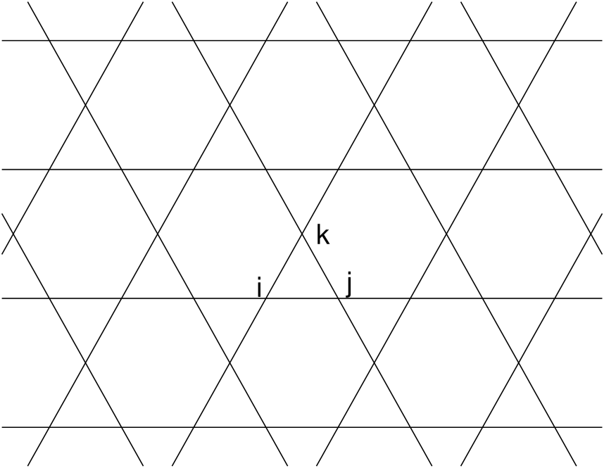
FIG. 1.: The kagomé lattice is a two-dimensional periodic array of equilateral triangles and regular hexagons. Sites $i,j,k$ are vertices of an elementary triangle.

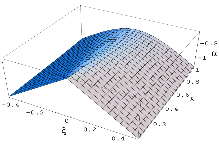
FIG. 2.: Phase boundary surface $x=x(\xi,\alpha)$ where $x$ is the reduced temperature, $\xi$ is the reduced magnetic field and $\alpha$ is the reduced anisotropy parameter. Figures 3-8 are projections of this surface onto the $\xi-\alpha$ and $\xi-x$ planes and will illustrate several unusual features of the surface. The reduced parameters $\xi=\tilde{\mu}h_{z}/J_{3}$, $\alpha={\mathcal{D}}/J_{3}$, $x=T/T_{c}$ where $k_{B}T_{c}/J_{3}=Q^{-1}_{3c}=0.25189\cdots$.

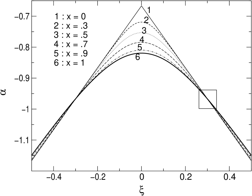
FIG. 3.: Isotherms in the $\xi$(magnetic field) $-$ $\alpha$(anisotropy) plane for several values of $x$(temperature), including the critical isotherm $x=1$. The existence of surface undulations in Figure 2 leads to the crossing of isotherms (boxed region). The reduced parameters $\xi=\tilde{\mu}h_{z}/J_{3}$, $\alpha={\mathcal{D}}/J_{3}$, $x=T/T_{c}$ where $k_{B}T_{c}/J_{3}=Q^{-1}_{3c}=0.25189\cdots$.

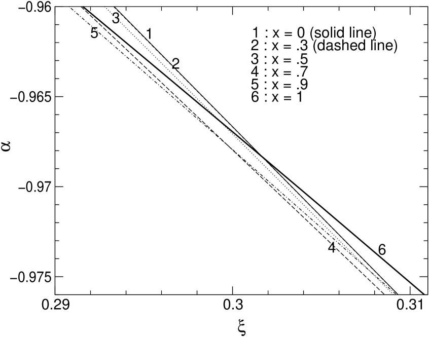
FIG. 4.: Boxed region in Figure 3 magnified to show details. The reduced parameters $\xi=\tilde{\mu}h_{z}/J_{3}$, $\alpha={\mathcal{D}}/J_{3}$, $x=T/T_{c}$ where $k_{B}T_{c}/J_{3}=Q^{-1}_{3c}=0.25189\cdots$.

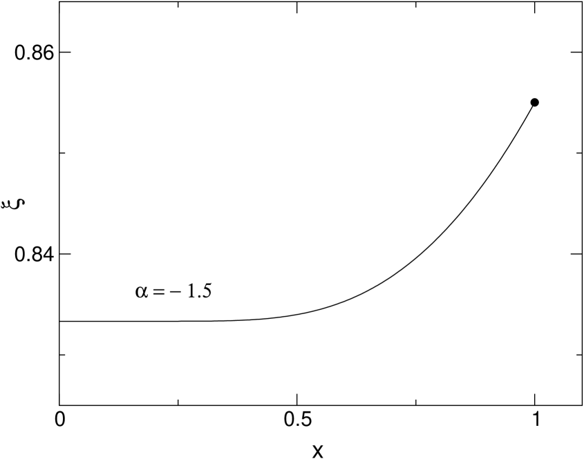
FIG. 5.: Projection of Figure 2 onto the $\xi$(magnetic field) $-$ $x$(temperature) plane for anisotropy parameter $\alpha=-1.5$ and $\xi>0$. The phase boundary curve is the locus of discontinuous transitions between the longitudinal upper phase and the transverse lower phase, and the solid circle is a critical point associated with a continuous transition. The reduced parameters $\xi=\tilde{\mu}h_{z}/J_{3}$, $\alpha={\mathcal{D}}/J_{3}$, $x=T/T_{c}$ where $k_{B}T_{c}/J_{3}=Q^{-1}_{3c}=0.25189\cdots$.

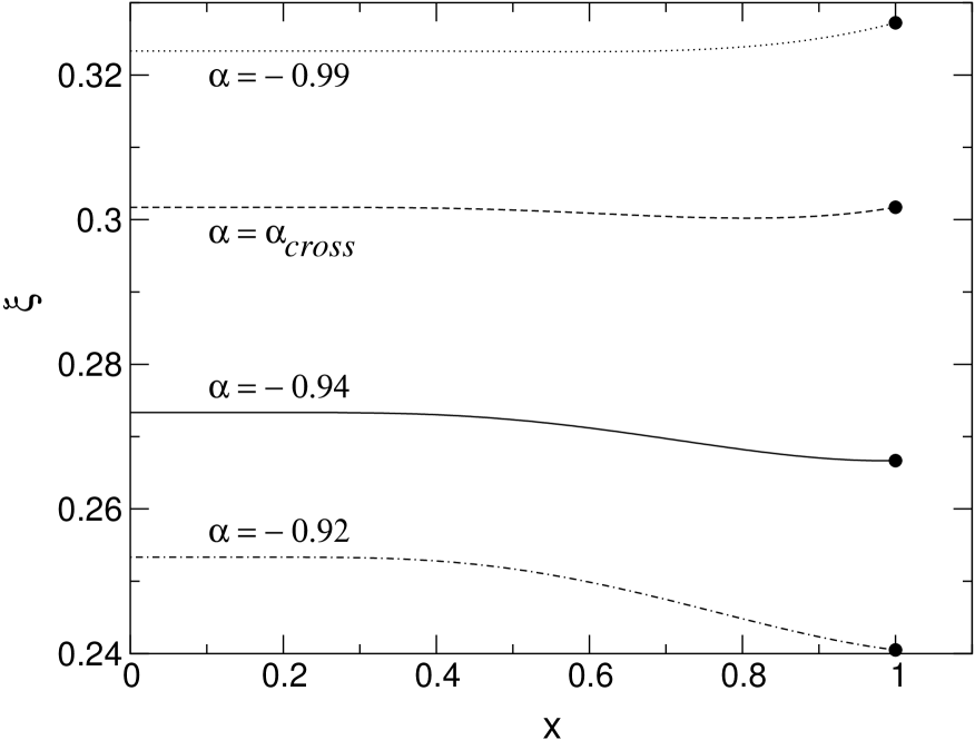
FIG. 6.: The $\xi$(magnetic field) $-$ $x$(temperature) phase boundary curves for values of the anisotropy parameter $\alpha$ where the curves change from being monotonically increasing to monotonically decreasing, via a non-monotonic region. At $\alpha_{cross}=-.96837\cdots$, the $x=0$ isotherm crosses the $x=1$ isotherm in the $\xi-\alpha$ plane. The reduced parameters $\xi=\tilde{\mu}h_{z}/J_{3}$, $\alpha={\mathcal{D}}/J_{3}$, $x=T/T_{c}$ where $k_{B}T_{c}/J_{3}=Q^{-1}_{3c}=0.25189\cdots$.

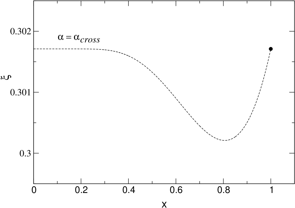
FIG. 7.: The curve $\alpha=\alpha_{cross}=-0.96837\cdots$ of Figure 6 magnified to show details of the nonmonotonicity. The reduced parameters $\xi=\tilde{\mu}h_{z}/J_{3}$, $\alpha={\mathcal{D}}/J_{3}$, $x=T/T_{c}$ where $k_{B}T_{c}/J_{3}=Q^{-1}_{3c}=0.25189\cdots$.

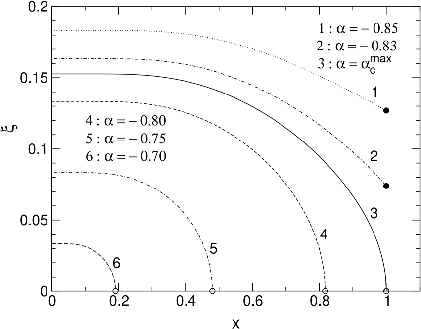
FIG. 8.: The $\xi$(magnetic field) $-$ $x$(temperature) phase boundary curves for several values of the anisotropy parameter $\alpha$ around $\alpha^{max}_{c}=-0.81929\cdots$. The figure extends symmetrically for $\xi<0$. Curves $1$ and $2$ end at solid circles representing critical points, while curves $4$, $5$ and $6$ end at open circles representing confluent singularities. For curve $3$, the critical point meets its reflective image critical point at the confluent-critical point (shaded circle). The reduced parameters $\xi=\tilde{\mu}h_{z}/J_{3}$, $\alpha={\mathcal{D}}/J_{3}$, $x=T/T_{c}$ where $k_{B}T_{c}/J_{3}=Q^{-1}_{3c}=0.25189\cdots$.

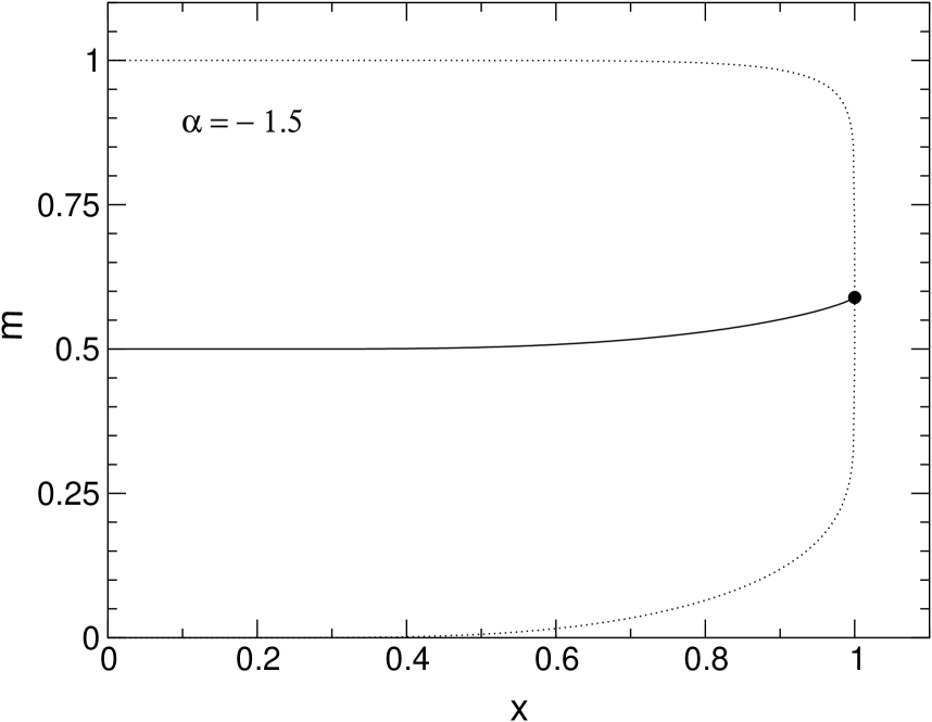
FIG. 9.: The longitudinal-transverse coexistence curve (dotted line) and the corresponding curvilinear diameter (solid line) for $\alpha=-1.5$ in the $m$(magnetization) $-$ $x$(temperature) plane. The coexistence curve is singular at its critical point (solid circle). The reduced parameters $m=<S_{i}>$, $\alpha={\mathcal{D}}/J_{3}$, $x=T/T_{c}$ where $k_{B}T_{c}/J_{3}=Q^{-1}_{3c}=0.25189\cdots$.

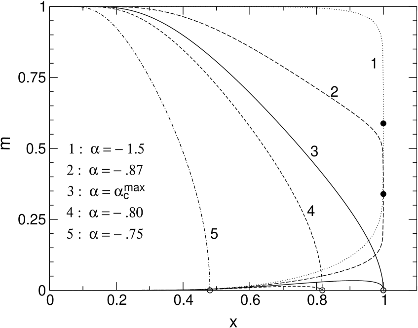
FIG. 10.: Longitudinal-transverse coexistence curves in the $m$(magnetization) $-$ $x$(temperature) plane for several values of $\alpha$ around $\alpha^{max}_{c}=-0.81929\cdots$. Solid circles are critical points, open circles are confluence points, and the shaded circle is a confluent-critical point. The figure extends symmetrically for $m<0$, so that curves $3$, $4$ and $5$ entrap homogeneous transverse phases within tadpole-shaped regions. No such trapped transverse phases exist for curves $1$ or $2$. The reduced parameters $m=<S_{i}>$, $\alpha={\mathcal{D}}/J_{3}$, $x=T/T_{c}$ where $k_{B}T_{c}/J_{3}=Q^{-1}_{3c}=0.25189\cdots$.

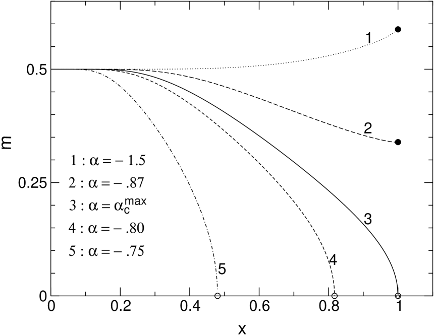
FIG. 11.: Curvilinear diameters corresponding to the coexistence curves of Figure 10, showing the diameters changing from monotonically increasing to monotonically decreasing behavior and ending either at a critical point (solid circle), or eventually at a confluence (open circle) point or a confluent-critical (shaded circle) point. The reduced parameters $m=<S_{i}>$, $\alpha={\mathcal{D}}/J_{3}$, $x=T/T_{c}$ where $k_{B}T_{c}/J_{3}=Q^{-1}_{3c}=0.25189\cdots$. The value $\alpha^{max}_{c}=-0.81929\cdots$.

REFERENCES

- [1] M. Blume, V.J. Emery and R. B. Griffiths, Phys. Rev. A 4, 1071 (1971).
- [2] M. Blume, Phys. Rev. 141, 517 (1966); H. W. Capel, Physica 32, 966 (1966); 33, 295 (1967); 37, 423 (1967).
- [3] See, e.g., M. Keskin and A. Solak, J. Chem. Phys. 112, 6396 (2000), and references cited therein; X. N. Wu and F. Y. Wu, J. Stat. Phys. 50, 41 (1988).
- [4] R. B. Griffiths, Physica 33, 689 (1967).
- [5] F. Y. Wu, Chinese J. Phys. 16, 153 (1978).
- [6] N. S. Sullivan, Bull. Mag. Reson. 11, 86 (1987) and references cited therein; M. Roger, J. J. Hetherington and J. M. Delrieu, Rev. Mod. Phys. 55, 1 (1983).
- [7] J.H. Barry and N.S. Sullivan, Int. J. Mod. Phys B 7, 2831 (1993).
- [8] See, e.g., R. B. Griffiths, in Phase Transitions and Critical Phenomena, vol. 1, ed. C. Domb and M. S. Green (Academic, New York, 1972); I. Syozi, ibid; R. J. Baxter, Exactly Solved Models in Statistical Mechanics, (Academic, New York, 1982).
- [9] R. J. Baxter and I. G. Enting, J. Phys. A 11, 2463 (1978); R. M. F. Houtappel, Physica 16, 425 (1950); S. Naya, Prog. Theor. Phys. 11, 53 (1954); R. J. Baxter, ref. 8; J. H. Barry, T. Tanaka, M. Khatun and C. H. Múnera, Phys. Rev. B 44, 2595 (1991).