Heat conduction in 1D lattices with on-site potential

Abstract

The process of heat conduction in one-dimensional lattice with on-site potential is studied by means of numerical simulation. Using discrete Frenkel-Kontorova, $\phi$–4 and sinh-Gordon we demonstrate that contrary to previously expressed opinions the sole anharmonicity of the on-site potential is insufficient to ensure the normal heat conductivity in these systems. The character of the heat conduction is determined by the spectrum of nonlinear excitations peculiar for every given model and therefore depends on the concrete potential shape and temperature of the lattice. The reason is that the peculiarities of the nonlinear excitations and their interactions prescribe the energy scattering mechanism in each model. For models sin-Gordon and $\phi$–4 phonons are scattered at thermalized lattice of topological solitons; for sinh-Gordon and $\phi$–4 - models the phonons are scattered at localized high-frequency breathers (in the case of $\phi$–4 the scattering mechanism switches with the growth of the temperature).

1 Introduction

Heat conductivity of 1D lattices is well known classical problem related to microscopic foundation of Fourier law. The problem started from the famous work of Fermi, Pasta and Ulam [1], where abnormal process of heat transfer has been detected in the first time. Non-integrability of the system is necessary condition for normal heat conductivity. As it was demonstrated recently for the FPU lattice [2, 3, 4], disordered harmonic chain [5, 6, 7], diatomic 1D gas of colliding particles [8, 9, 10] and the diatomic Toda lattice [11], the non-integrability is not sufficient in order to get normal heat conductivity. It leads to linear distribution of the temperature along the chain, but the value of heat flux is proportional to $1/N^{\alpha}$, where $0<\alpha<1$ and $N$ is the number of particles in the chain. Thus, the coefficient of the heat conductivity diverges in thermodynamical limit $N\rightarrow\infty$. Analytical estimations [4] have demonstrated that any chain possessing acoustic phonon branch should have infinite heat conductivity in the limit of low temperatures.

From the other side, there are some artificial systems with on-site potential having normal heat conductivity [12, 13]. Heat conductivity of Frenkel-Kontorova chain in the first time was considered in paper [14]. Finite heat conductivity for certain set of parameters was obtained for Frenkel-Kontorova chain [15], for the chain with sinh-Gordon on-site potential [16] and for the chain with $\phi^{4}$ on-site potential [17, 18]. These models are not invariant with respect to translation and the momentum is not conserved. It was supposed that the on-site potential is extremely significant for normal heat conduction [17] and that the anharmonicity of the on-site potential is sufficient to ensure the validity of Fourier law [19]. Detailed review of the problem is presented in recent paper [20].

Peculiarities of the heat conduction of the Frenkel-Kontorova model for complete set of parameters and temperature of the system are not known. The chains with zero average pressure were demonstrated to have normal heat conductivity [21, 22, 23]. In papers [22, 23] the transition from abnormal to normal heat conductivity has been detected at certain temperature. Paper [20] contains detailed review of the heat conductivity peculiarities in 1D molecular systems.

There are no detailed investigations similar to mentioned above and concerning the properties of the chains with on-site potential in the whole temperature range. As it was mentioned above, there exists certain incompleteness of the knowledge concerning even the most popular and paradigmatic discrete Frenkel-Kontorova chain. This lattice is of special interest as its continuous counterpart is famous sin-Gordon system (having, of course, divergent heat conductivity). The transition between two regimes with the growth of temperature is expected for discrete system; however it may be dependent also on other parameters of the lattice

The question of special interest is also the mechanism of heat flow scattering which gives rise to finite heat conductivity. For the chain with periodic nearest-neighbor interaction it was demonstrated [22, 23] that the transition to normal heat conductivity corresponds to abrupt growth of concentration of rotation solitons (rotobreathers), demonstrating certain similarity with phase transition. Namely, the region of the transition temperature corresponds to maximum region of the heat capacity of the lattice. Similarly, it is reasonable to suppose that every lattice with finite heat conductivity has its peculiar mechanism of scattering the heat flow.

The paper is devoted to the detailed simulation of the discrete lattices with on-site nonlinearity and quadratic potential of nearest-neighbor interaction and investigation of their heat conductivity. The lattices are Frenkel-Kontorova, sinh-Gordon, and discrete $\phi$-4. For every case the dependence of the heat conductivity on the temperature and parameters of the lattice will be explored and concrete elementary excitation responsible for the change of regimes will be revealed.

2 Description of the model

Let us consider one-dimensional atomic chain arranged along $x$ axis. All particles are of equal mass $M$, and the nearest-neighbor interaction is described by harmonic potential having rigidity $K$. Then the Hamiltonian of the lattice will take a form

$${\cal H}=\sum_{n}\{\frac{1}{2}M\dot{x}_{n}^{2}+\frac{1}{2}K(x_{n+1}-x_{n})^{2}+U(x_{n})\},$$ (1)

where the dot denotes the differentiation with respect to time $t$, $x_{n}$ is the displacement of the $n$-th particle from its equilibrium position and $U(x)$ is the on-site potential.

The dimensionless variables are introduced as $u_{n}=2\pi x_{n}/a$ ($a$ is the equilibrium distance between the particles) for the displacement, $\tau=t\sqrt{K/M}$ for the time and $H=4\pi^{2}{\cal H}/Ka^{2}$ for the energy. Hamiltonian (1) takes the form

$$H=\sum_{n}\{\frac{1}{2}{u^{\prime}_{n}}^{2}+\frac{1}{2}(u_{n+1}-u_{n})^{2}+V(u_{n})\},$$ (2)

where the stroke denotes the differentiation with respect to the dimensionless time $\tau$ and the dimensionless on-site potential is introduced as $V(u_{n})=4\pi^{2}U(au_{n}/2\pi)/Ka^{2}$. Natural definition for the dimensionless temperature is $T=4\pi^{2}k_{B}\Theta/Ka^{2}$, where $k_{B}$ is Boltzmann constant and $\Theta$ is the temperature in common units.

We are going to consider four widely used models for on-site potential: harmonic potential

$$V(u)=\frac{1}{2}\omega_{0}^{2}u^{2};$$ (3)

sin-Gorgon potential

$$V(u)=\epsilon[1+\cos(u)];$$ (4)

$\phi$-4 potential

$$V(u)=2\epsilon[(u/\pi)^{2}-1]^{2}$$ (5)

and sinh-Gordon potential

$$V(u)=\omega_{0}^{2}[\cosh(u)-1].$$ (6)

Parameter $\epsilon>0$ determines the value of potential barrier between neighboring wells and its inverse $g=1/{\epsilon}$ characterizes the cooperativeness of the system. Potentials (4) and (5) have the same distance between neighboring wells equal to 2$\pi$ and equal value of the potential barrier 2$\epsilon$. Parameter $\omega_{0}$ in (3) and (6) corresponds to minimal frequency of harmonic vibrations of the lattice.

3 Methods for computation of the heat conduction coefficient

The goal is to simulate the process of heat conduction in finite chain containing N particles. For this sake the left side of the chain ($n\leq 0$) has to be connected to a thermostat with temperature $T_{+}$, and the right side ($n>N$) – to a thermostat with temperature $T_{-}$ ($T_{+}>T_{-}$). For the sake of the simulation we consider the chain of $N_{-}+N+N_{+}$ particles, where the first $N_{+}$ particles are attached to the thermostat $T_{+}$, an the last $N_{-}$ particles – to the thermostat $T_{-}$ (Fig. 1). The potential of the nearest-neighbor interaction is harmonic, therefore the equilibrium length of the chain does not depend on the temperature. It implies that the boundary conditions at the ends of the lattice has no noticeable effect on the process of the heat conduction and both the conditions of free (Fig.1 (a)) and fixed (Fig. 1 (b)) may be used. Numerical simulations with $N_{\pm}=40$ has demonstrated the absence of the effect depending on concrete choice of the boundary conditions. We’ll use the condition of free ends with $N_{\pm}=40$ for all simulations.

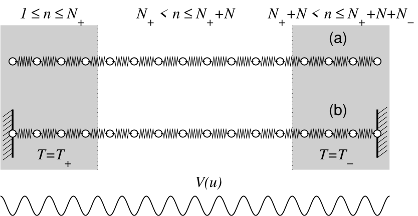
Figure 1: Model of the chain of $N_{+}+N+N_{-}$ particles with left $N_{+}$ particles attached to $T=T_{+}$ thermostat and right $N_{-}$ particles attached to $T=T_{-}$ thermostat. Boundary conditions correspond to free (a) and fixed (b) end particles. The potential $V(u)$ corresponds to discrete Frenkel - Kontorova model.

Majority of papers devoted to the topic of the heat conduction [2, 3, 15, 17] uses deterministic Nose - Hoover thermostat [24] with $N_{+}=N_{-}=1$. However this thermostat has been designed for the description of the equilibrium thermalized system and is not universally suitable for the description of non-equilibrium processes. Therefore our choice is well-known stochastic Langevin thermostat. Detailed comparison of these two thermostats is presented in Appendix 9.3.

Let us consider the chain with free ends ($1<n<N+N_{+}+N_{-}$) with $N_{\pm}$ particles at both ends attached to Langevin thermostats. The dynamics of the system is described by equations

$$u^{\prime\prime}_{n} = u_{n+1}-u_{n}-F(u_{n})-\gamma u^{\prime}_{n}+\xi_{n}^{+},$$

$$n = 1,$$

$$u^{\prime\prime}_{n} = u_{n+1}-2u_{n}+u_{n-1}-F(u_{n})-\gamma u^{\prime}_{n}+\xi_{n}^{+},$$

$$n = 2,...,N_{+},$$

$$u^{\prime\prime}_{n} = u_{n+1}-2u_{n}+u_{n-1}-F(u_{n}),$$ (7)

$$n = N_{+}+1,...,N_{+}+N,$$

$$u^{\prime\prime}_{n} = u_{n+1}-2u_{n}+u_{n-1}-F(u_{n})-\gamma u^{\prime}_{n}+\xi_{n}^{-},$$

$$n = N_{+}+N+1,...,N_{+}+N+N_{-}-1,$$

$$u^{\prime\prime}_{n} = u_{n-1}-u_{n}-F(u_{n})-\gamma u^{\prime}_{n}+\xi_{n}^{-},$$

$$n = N_{+}+N+N_{-},$$

where $F(u)=dU(u)/du$, the damping coefficient $\gamma=1/\tau_{r}$, $\tau_{r}$ is the characteristic relaxation time of the particles attached to the thermostat, $\xi_{n}^{\pm}$ is the random external force corresponding to Gaussian white noise normalized as

$$\langle\xi_{n}^{\pm}(\tau)\rangle=\langle\xi_{n}^{\pm}(\tau_{1})\xi_{k}^{\mp}(\tau_{2})\rangle=0,$$

$$\langle\xi_{n}^{\pm}(\tau_{1})\xi_{k}^{\pm}(\tau_{2})\rangle=2\gamma T_{\pm}\delta_{nk}\delta(\tau_{2}-\tau_{1}).$$

Details of numeric realization of the Langevin thermostat and random forces are presented in Appendix 9.1.

At every moment the dimensionless temperature of the $n$-th particle $t_{n}(\tau)={u^{\prime}_{n}}^{2}(\tau)$. In order to determine the value of the local heat flux $j_{n}$ the energy distribution among the particles of the chain is considered:

$$h_{n}=\frac{1}{2}\left[\frac{1}{2}({u^{\prime}_{n}}^{2}+{u^{\prime}_{n+1}}^{2})+V(u_{n})+V(u_{n+1})+(u_{n+1}-u_{n})^{2}\right].$$ (8)

By differentiating equation (8) with respect to time $\tau$ we get

$$h^{\prime}_{n}=\frac{1}{2}\left\{u^{\prime}_{n}[u^{\prime\prime}_{n}+F(u_{n})]+u^{\prime}_{n+1}[u^{\prime\prime}_{n+1}+F(u_{n+1})]\right\}+(u_{n+1}-u_{n})(u^{\prime}_{n+1}-u^{\prime}_{n}).$$

With account of (7) we obtain

$$h^{\prime}_{n}=\frac{1}{2}\left[u^{\prime}_{n+1}(u_{n+2}-u_{n})-u^{\prime}_{n}(u_{n+1}-u_{n-1})\right].$$ (9)

Taking into account the continuity condition $h^{\prime}_{n}=j_{n}-j_{n-1}$ we get the expression for the energy flux: $j_{n}=-u^{\prime}_{n}(u_{n+1}-u_{n-1})/2$.

System of equations (7) has been integrated numerically. We used the values of $\gamma=0.1$, $N_{\pm}=40$, $N=10$, 20, 40, 80, 160, 320, 640 and initial conditions corresponding to the ground state of the chain. After the time $\tau=10^{5}$ has elapsed, the end particles achieved thermal equilibrium with the thermostat and stationary heat flux has been formed. Afterwards the dynamics of system (7) has been simulated at the time scale of order $\tau=10^{7}$. The average temperatures of the particles

$$T_{n}=\langle t_{n}(\tau)\rangle_{\tau}=\lim_{\tau\rightarrow\infty}\frac{1}{\tau}\int_{0}^{\tau}{u^{\prime}_{n}}^{2}(s)ds.$$ (10)

and average values of the heat flux

$$J_{n}=\langle j_{n}(\tau)\rangle_{\tau}=\lim_{\tau\rightarrow\infty}\frac{1}{\tau}\int_{0}^{\tau}j_{n}(s)ds.$$ (11)

were computed for the fragment of the chain between the thermostats.

If the temperature gradient $\Delta T=T_{+}-T_{-}$ is small, this method allows avoiding the temperature jumps at the ends of the free fragment of the chain [26]. Characteristic distributions of the heat flux $J_{n}$ and local temperature $T_{n}$ are demonstrated at Fig. 2. At the inner fragment of the chain $N_{+}<n\leq N_{+}+N$ the heat flux is constant $(J_{n}=J)$ and the temperature profile is linear. The coefficient of the heat conductivity is determined using the information concerning the inner fragment of the chain:

$$\kappa(N)=J(N-1)/(T_{N_{+}+1}-T_{N_{+}+N}).$$ (12)

If the function $T=\alpha n+b$ is the best linear approximation for $T=T_{n}$ data at the inner fragment of the chain $N_{+}<n\leq N_{+}+N$, then the value $\kappa(N)$ may be calculated with better accuracy by taking $\kappa(N)=J\alpha$.

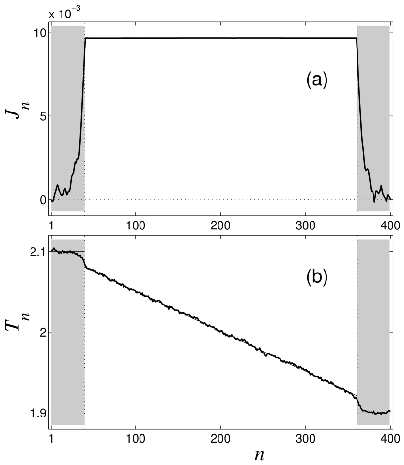
Figure 2: Distribution of the local heat flux $J_{n}$ (a) and local temperature $T_{n}$ (b) in the chain with periodic on-site potential (4), $\epsilon=1$, $N=320$, $N_{\pm}=40$, $T_{+}=2.1$, $T_{-}=1.9$. Time of averaging $\tau=10^{7}$. Fragments of the chain interacting with the thermostats are embedded in gray.

Limit value

$$\kappa=\lim_{N\rightarrow\infty}\kappa(N)$$ (13)

will correspond to the coefficient of the heat conductivity at temperature $T=(T_{+}+T_{-})/2$. The question regarding the finiteness of the heat conductivity is reduced to the existence of finite limit (13). I the sequence $\kappa(N)$ diverges as $N\rightarrow\infty$ then the chain has infinite heat conductivity at this value of the temperature.

Alternative way to compute the heat conductivity $\kappa$ is related to well-known Green-Kubo formula [27]:

$$\kappa=\lim_{\tau\rightarrow\infty}\int_{0}^{\tau}\lim_{N\rightarrow\infty}\frac{1}{NT^{2}}\langle{\bf J}(s){\bf J}(0)\rangle ds~{},$$ (14)

where $N$ is already the number of particles in the chain with periodic boundary conditions,

$${\bf J(\tau)}=\sum_{n=1}^{N}j_{n}(\tau)$$

is the general heat flux and the averaging $\langle\cdot\rangle$ is performed over all thermalized states of the chain. Consequently, the finiteness of the heat conductivity is related to the convergence of the integral

$$\int_{0}^{\infty}C(\tau)d\tau,$$ (15)

e.g. to the evaluation of the descending rate of the function

$$C(\tau)=\lim_{N\rightarrow\infty}\frac{1}{NT^{2}}\langle{\bf J}(\tau){\bf J}(0)\rangle.$$

Numerically the above autocorrelation function may be found only for finite chain

$$C_{N}(\tau)=\frac{1}{NT^{2}}\langle{\bf J}(s){\bf J}(s-\tau)\rangle_{s}.$$ (16)

For large enough values of $N$ the correlation function $C_{N}(\tau)$ is believed to approximate the function $C(t)$ with acceptable accuracy. In order to get stable results the value $N=4000$ is usually sufficient. More details concerning the computation of the autocorrelation function are presented in Appendix 9.2.

The methods for computing the heat conductivity coefficient (13), (14) are complementary and allow mutual verification of the results.

4 Heat conductivity of the chain with harmonic on-site potential

The chain with harmonic on-site potential (3) is described by linear equations and therefore is completely integrable. The energy transport is performed by non-interacting phonon modes. The heat flux $J$ does not depend on the chain length $N$, but only on the temperature difference $\Delta T$. Linear thermal profile is not formed. At the inner part of the chain the temperature is nearly constant $T_{n}=(T_{+}+T_{-})/2$ (Fig. 3). Therefore according to (12), the heat conductivity coefficient diverges. Correspondingly, the average correlation function $C(\tau)$ is constant and integral (15) diverges.

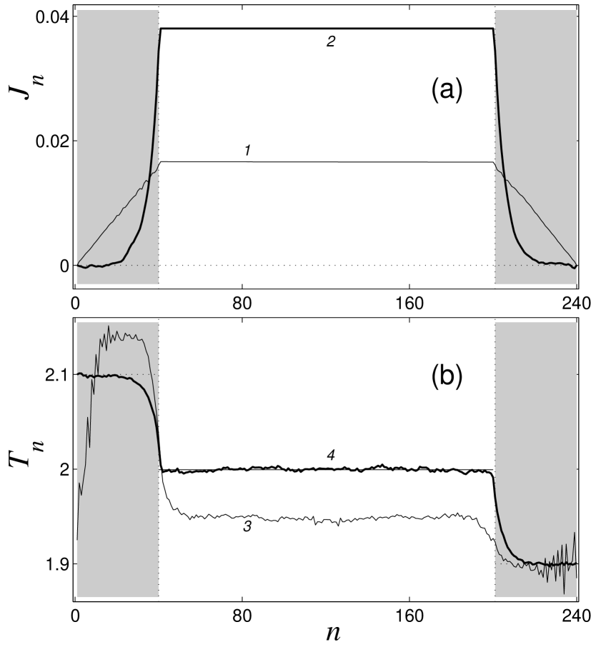
Figure 3: Distribution of local heat flux $J_{n}$ (a) and local temperature $T_{n}$ (b) in the chain with harmonic on-site potential (3), $\omega_{0}=1$, $N=160$, $N_{\pm}=40$, $T_{+}=2.1$, $T_{-}=1.9$, averaging time $\tau=10^{7}$. The fragments of the chain interaction with the thermostats are embedded in grey. Thin lines (1, 3) are obtained by using the Nose-Hoover thermostat with $\tau_{r}=1$, and thick (2, 4) – by using the Langevine thermostat with $\tau_{r}=10$.

5 Heat conduction of the chain with periodic on-site potential

Characteristic features of dynamics of the chain with periodic on-site potential (4) depend on the values of the temperature. As the temperature is small $T\ll\epsilon$, the on-site potential may be approximated by harmonic single-well potential (3) with $\omega_{0}=\sqrt{\epsilon}$. The heat transport is governed by weakly interacting phonons. At the temperature $T\sim\epsilon$ the chaotic superlattice of topological solitons is formed and the transport properties change drastically. At very high temperatures $T\gg\epsilon$ the chain is effectively detached from the site and again weakly interacting phonons govern the heat transport. Therefore it is reasonable to investigate the dependence of the heat conductivity on the reduced temperature $\tilde{T}=T/\epsilon$.

The behavior of the chain also depends on the cooperativeness parameter $g=1/\epsilon$. The more the cooperativeness, the less is the density of the soliton superlattice and the phonon scattering effects are less significant. The limit $g\rightarrow\infty$ ($\epsilon\rightarrow 0$) corresponds to completely integrable continuum sin-Gordon equation.

Generally, three limits of discrete Frenkel-Kontorova system correspond to completely integrable systems: at $\tilde{T}\rightarrow 0$ the system reduces to the harmonic chain with harmonic on-site potential; at $\tilde{T}\rightarrow\infty$ – to isolated harmonic chain; at $g\rightarrow\infty$ – to continuum sin-Gordon equation. All these limit systems have diverging heat conductivity. The behavior of the system in the vicinity of these limits is a natural question to be addressed.

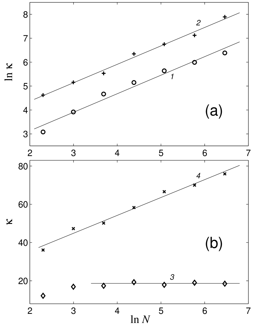
Figure 4: Dependence of the logarithm of the heat conductivity coefficient $\ln\kappa(N)$ (a) and $\kappa(N)$ (b) on the logarithm of the inner fragment length $\ln N$ ($N_{+}=N_{-}=40$) for the chain with periodic on-site potential (4), $\epsilon=1$, $T=0.2$ (markers 1), $T=200$ (markers 2), $T=3$ (markers 3) and $T=20$ (markers 4). The markers denote the computed values and the lines correspond to the best linear approximations.

Let us start from $g=1$ $(\epsilon=1$, $\tilde{T}=T)$ and investigate the sequence $\kappa(N)$ as $N$ grows $(N=10,$ 20, 40, 80, 160, 320, 640) and different values of $T$. As it is may be suggested from Fig. 4 at small ($T=0.2$) and large ($T=200$) temperatures the heat conductivity coefficient $\kappa(N)$ grows as $N^{\alpha}$, at $T=20$ – as $\ln N$, and at $T=3$ converges to finite value $\kappa=18.5$. Therefore it may be concluded that at $T=3$ the chain has finite heat conductivity. The data related to the other values of the temperature does not allow to draw any conclusions about the behavior of the heat conductivity at larger values of $N$. Generally speaking, it may happen that for longer chains $\kappa(N)$ will attain certain finite value. Computational tools we use do not allow to investigate higher values of $N$. Stil, it is possible to get additional information from the behavior of the autocorrelation function $C(\tau)$ at $\tau\rightarrow\infty$.

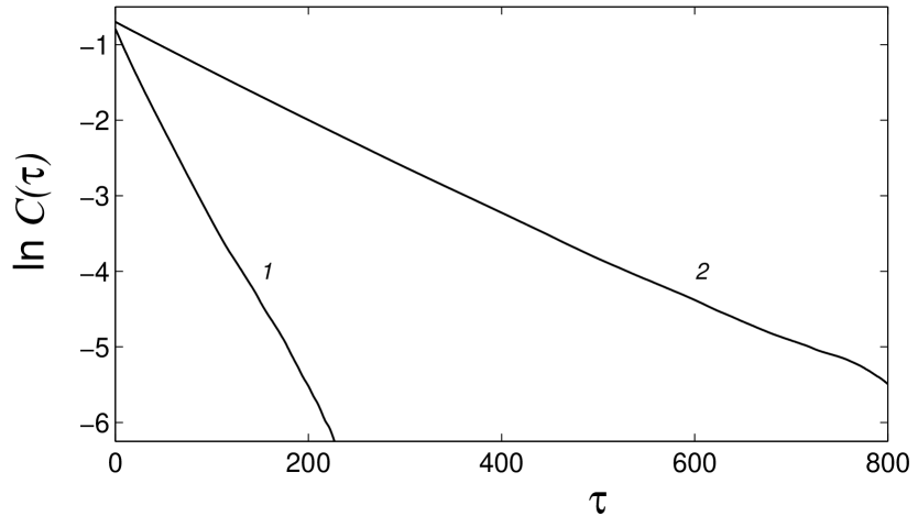
Figure 5: Exponential decrease of the autocorrelation function $C(\tau)$ in the chain with periodic on-site potential (4), $\epsilon=1$, $T=3$ (curve 1) and $T=20$ (curve 2) (semilogarythmic coordinates).

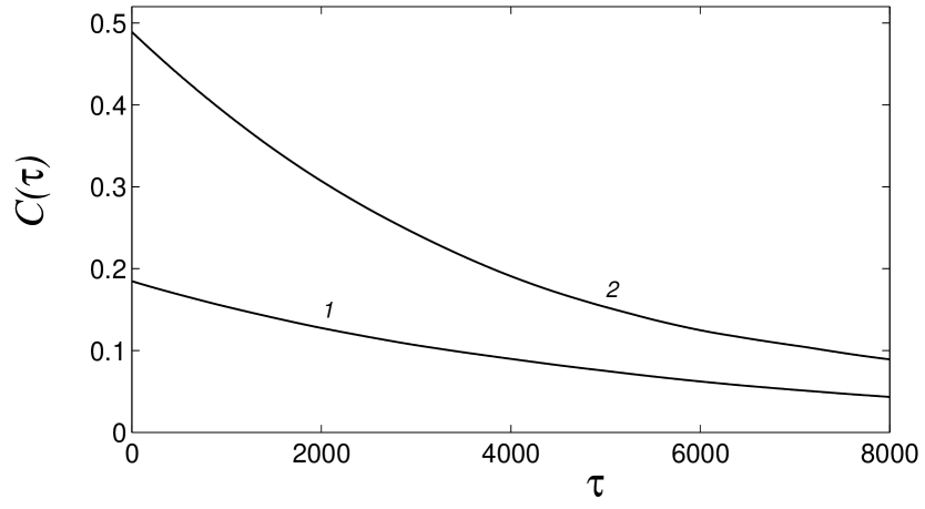
Figure 6: Autocorrelation functions $C(\tau)$ in the chain with periodic on-site potential (4), $\epsilon=1$, $T=0.2$ (curve 1) and $T=200$ (curve 2).

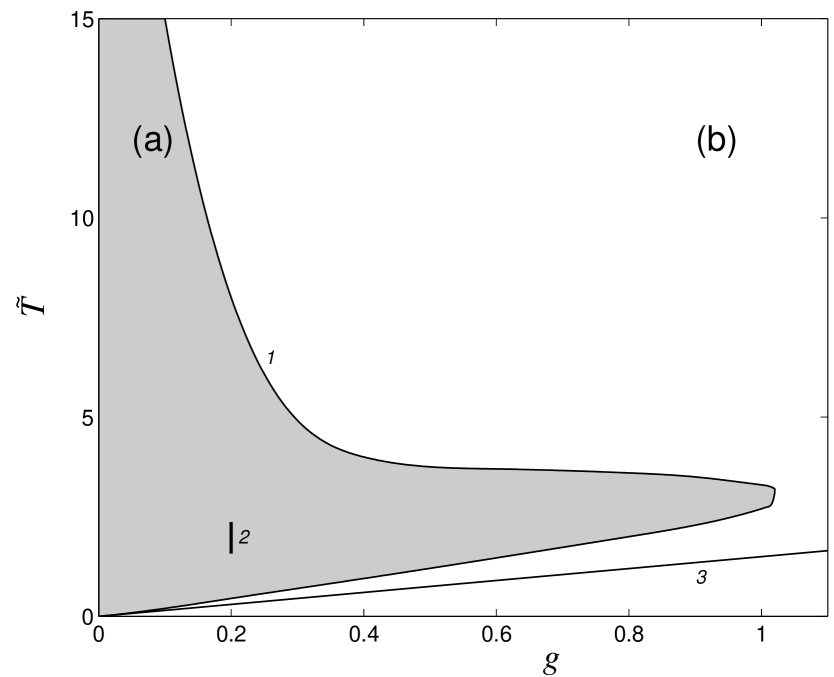
Figure 7: The zone in the space of parameters $(g,\tilde{T})$, where for finite chains of length $N\leq 640$ with on-site potential (4) he heat conductivity converges (a, grey zone) and diverges (b, white zone). Curve 1 divides these two zones. Interval 2 corresponds to the parameters used in [15]. For finite chains $(N\leq 640)$ with on-site potential $\phi$–4 (5) finite heat conductivity is detected only above line 3.

Numerical simulation demonstrates that for $T=3$ the autocorrelation function decreases exponentially (Fig. 5, curve 1). Integral (15) converges and the Green-Kubo formula (14) gives $\kappa=17.5$, in good correspondence with $\kappa=18.5$ obtained from direct simulation of the heat flux. At $T=20$ the autocorrelation function at time scale $0\leq\tau\leq 800$ also decreases exponentially (Fig. 5, curve 2). If this trend will persist also for $\tau>800$, the Green-Kubo formula will give $\kappa=77.4$. It is reasonable to compare this value with the result for $\kappa(N)$ presented at Fig. 4 (curve 4). Maximum value of $\kappa(640)=75.9$ and no trend towards any finite limit of $\kappa(N)$ may be detected. Therefore the likely result is divergence. In order to verify this result the simulation for larger values of $N$ (1280, 2560, 5120, 10240) is required, which is beyond our computational possibilities.

The problem for $T=0.2$ and $T=200$ is even more difficult. The autocorrelation function is presented at Fig. 6. The decrease of the function is very slow and no unambiguous conclusion concerning its character may be drawn out. While extrapolating $c(\tau)$ for $\tau>8000$ by exponent, the Green-Kubo formula yields $\kappa=1016$ for $T=0.2$ and $\kappa=2252$ for $T=200$. In order to get additional information another consuming simulation is required. Still, from the other side, for $T=200$ at $N=640$ the logarithm of the heat conductivity $\ln\kappa(N)=7.9>\ln(2252)=7.7$, and the dependence $\ln\kappa(N)$ (Fig. 4, curve 2) does not demonstrate any trend towards convergence. Therefore the most likely result in this case is also the divergence of the heat conductivity.

Let us consider the sequence $\kappa(N)$ ($N=10$, 20, 40, 80, 160, 320, 640) at other values of the cooperativeness. The results are summarized at Fig. 7. The space of parameters $(g,\tilde{T})$ is divided to two zones denoted by different colors. In the first (gray) zone the sequence $\kappa(N)$ converges ($\kappa(160)\approx\kappa(320)\approx\kappa(640)$), and in the second (white) zone the sequence grows monotonously. Then, in the first zone Frenkel-Kontorova model has finite heat conductivity, and in the second zone the heat conductivity is either divergent or finite but very high (for $N\leq 640$ the Fourier law is not valid).

The first zone is limited by certain finite value of $g$: for some $g_{0}>1$ and for all $g>g_{0}$ no convergence of $\kappa(N)$ was detected. The explanation is that for growing $g$ the system becomes closer to continuum integrable sin-Gordon equation. At any fixed $g<g_{0}$ for $N\leq 640$ the heat conductivity converges only for some finite temperature interval $0<\tilde{T}_{b}<\tilde{T}<\tilde{T}_{h}<\infty$. As the cooperativeness decreases ($g\rightarrow 0$), the upper boundary of this interval tends to infinity ($\tilde{T}_{h}\rightarrow\infty$), and the lower boundary tends to zero ($\tilde{T}_{b}\rightarrow 0$) proportionally to $g$.

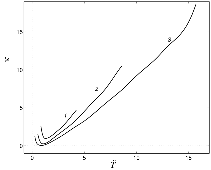
Figure 8: Dependence of the heat conductivity coefficient $\kappa$ from the reduced temperature $\tilde{T}=T/\epsilon$ for the chain with periodic on-site potential (4) for $\epsilon=3$ (curve 1), $\epsilon=5$ (curve 2) and $\epsilon=10$ (curve 3).

The dependence of $\kappa$ on the reduced temperature $\tilde{T}$ is presented at Fig. 8. Within the interval $[\tilde{T}_{b},\tilde{T}_{h}]$ there exists a critical value $\tilde{T}_{m}$ corresponding to the minimum of heat conductivity.

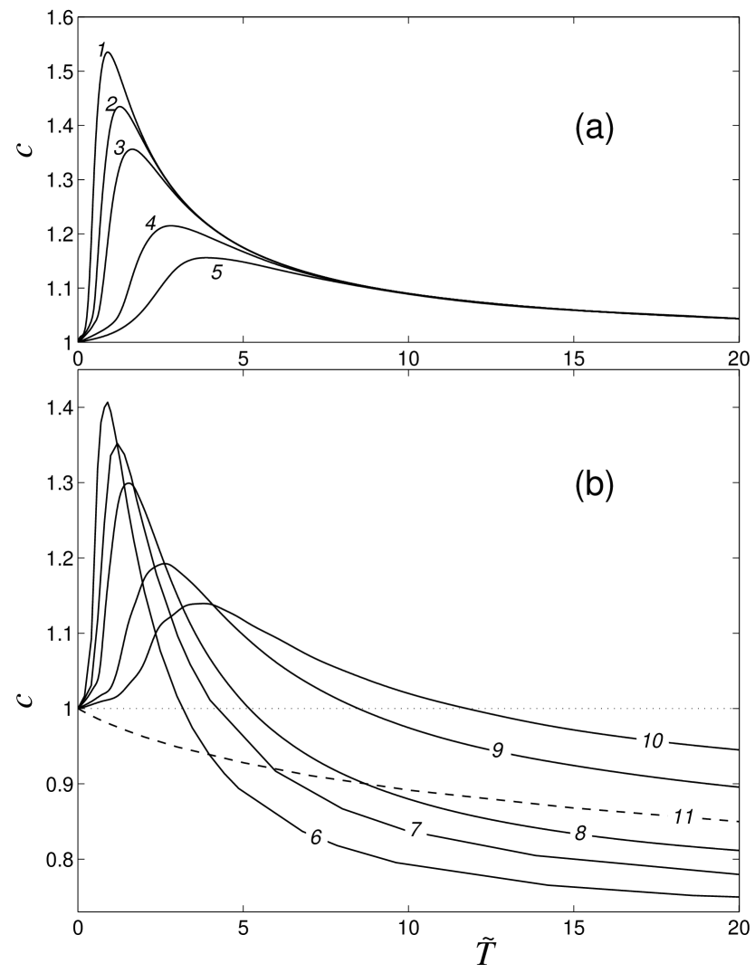
Figure 9: The dependence of the dimensionless heat capacity $c$ on the reduced temperature $\tilde{T}=T/\epsilon$ (a) for the chain with periodic on-site potential (4) and (b) for the chain with $\phi$–4 potential (5) for $\epsilon=10$ (curves 1,6), $\epsilon=5$ (curves 2, 7), $\epsilon=3$ (curves 3, 8), $\epsilon=1$ (curves 4, 9) and $\epsilon=0.5$ (curves 5, 10). Dashed curve 11 gives similar dependence for the chain with on-site sinh-Gordon potential (6), for $\omega_{0}=1$.

In order to reveal the mechanism of the heat conduction it is reasonable to explore the behavior of heat capacity $c=\langle H\rangle/NT$ ($\langle H\rangle$ is the average energy of cyclic $N$-atomic chain at the temperature $T$) on the reduced temperature $\tilde{T}$ (Fig. 9). The heat capacity of classic harmonic chain is always unity, therefore the discrepancy of this value from unity characterizes the significance of nonlinear effects at given temperature. The lattice considered has negative anharmonism and therefore its heat capacity must be more than unity for all temperature diapason. The heat capacity tends to unity as $\tilde{T}\rightarrow 0$ and $\tilde{T}\rightarrow\infty$ and has single maximum at certain temperature $\tilde{T}_{c}$. This value fairly coincides with the temperature $\tilde{T}_{m}$, which corresponds to the minimum of the heat conductivity.

Moreover, the increase and decrease of the heat capacity is clearly correlated with the decrease and increase of the heat conductivity respectively. This fact allows suggesting the same physical effects as responsible for both processes. For zero temperature the heat capacity is equal to unity. The increase of the heat capacity at higher temperatures is related to thermal activation of topological solitons (kinks and antikinks) which represent additional degrees of freedom for this system. As a result the dynamical superlattice of solitons appears. The density of this superlattice approaches its maximum at the temperature $\tilde{T}_{m}$. Further growth of the temperature results in the decrease of the number of degrees of freedom, which is manifested as effective detaching of the chain from the on-site potential. Therefore the heat capacity decreases and tends to unity as the temperature grows.

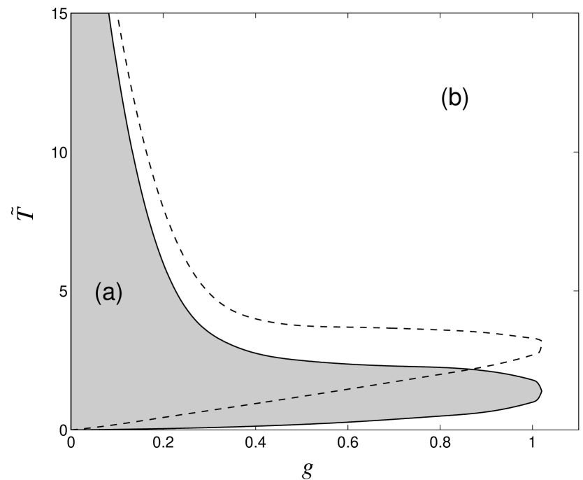
Figure 10: Zones in the space of parameters $(g,\tilde{T})$, where for finite chains $N\leq 640$ with periodic on-site potential (4) and period $l=2\pi\sqrt{2}$ the heat conductivity is normal (a, gray) and abnormal (b, white). Dashed line denotes the same boundary for commensurate Frenkel-Kontorova model ($l=2\pi$).

Correlations between the behavior of the heat capacity and the heat conductivity and especially fair coincidence of $\tilde{T}_{m}$ and $\tilde{T}_{c}$ allow us to suppose that the heat transfer is limited by phonon scattering on the soliton superlattice. The effectiveness of such scattering depends on the density of the superlattice as well as on the ability of single kink to scatter phonons. In the strongly cooperative regime $g>g_{0}$ the interaction between solitons and phonons is nearly elastic (close to the case of complete integrability) and therefore the heat conductivity has the trend to diverge. For lower cooperativeness the soliton-phonon interaction is less elastic and finite temperature diapason $[\tilde{T}_{b},\tilde{T}_{h}]$ of converging heat conductivity appears. For the cases of low $\tilde{T}<\tilde{T}_{b}$ and high $\tilde{T}>\tilde{T}_{h}$ temperatures the convergence of the heat conductivity cannot be detected in the framework of current experiment. The suggested reason of this effect is that the soliton superlattice effectively disappears.

Let us consider now incommensurate Frenkel - Kontorova chain where the period of the chain is different from the period of on-site potential. The dimensionless on-site potential is periodic function(4) with period $2\pi$, and the chain has period $l=2\pi q$. Then in system of equations (7) function $F(u_{n})$ will take the form

$$F(u_{n})=\frac{d}{du}U(u_{n}+nl).$$

For the sake of simulation we choose $q=l/2\pi=\sqrt{2}$, corresponding in certain sense to extremely incommensurate case. It is well-known [28] that such a lattice in its ground state already has soliton superlattice of nonzero density. Therefore the convergence of the heat conductivity is expected to be facilitated as compared to the commensurate case.

Fig. 10 demonstrates the zone in the space of parameters $(g,\tilde{T})$ where the sequence $\kappa(N)$, $N=10$, 20, 40, 80, 160, 320, 640. converges. For the sake of comparison the boundary for the commensurate case is also presented ($l=2\pi$). The result is than no qualitative change of the behavior occurs. The only difference is that the zone with normal heat conductivity moves downwise. This effect is related to presence of superlattice of solitons at any temperature. The transition to normal heat conduction occurs at lower temperature since less solitons should be thermally activated in order to achieve convergence. From the other side, the soliton superlattice facilitates effective detachment of the lattice from the on-site potential (the average coupling energy in the ground state is less) and therefore the upper boundary for the normal heat conduction is also achieved at lower temperatures.

6 Heat conductivity of the chain with double-well on-site potential

Let us consider the heat conductivity of the chain with on-site potential $\phi$-4 (5). For this case the analysis of the sequence $\kappa(N)$, $N=10$, 20, 40, 80, 160, 320, 640, demonstrates that the heat conductivity converges as $\tilde{T}>\tilde{T}_{0}=3g/2$ ($T>1.5$) - see Fig. 7.

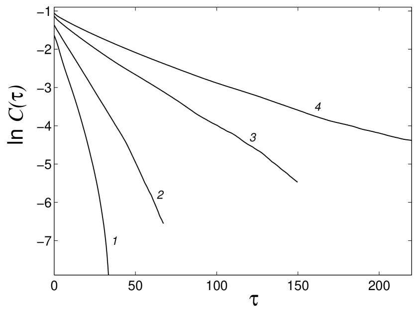
Figure 11: Exponential decrease of the autocorrelation function $C(\tau)$ in the chain with on-site potential $\phi$–4 (5), $\epsilon=1$, $T=20$ (curve 1), $T=10$ (curve 2), $T=5$ (curve 3) and $T=3$ (curve 4). (Semilogarythmic coordinates $\ln C(\tau)$ versus $\tau$).

In order to investigate the character of the heat conduction in the temperature range $\tilde{T}<\tilde{T}_{0}$ let us consider the temperature behavior of the autocorrelation function $C(\tau)$. For $g=1$ ($\epsilon=1$) this behavior is demonstrated at Fig. 11. As $\tau\rightarrow\infty$ the autocorrelation function decreases exponentially. The decrease rate grows as the temperature increases and therefore the conclusion concerning finite heat conductivity at $\tilde{T}>\tilde{T}_{0}$ is confirmed. At lower temperatures the decrease rate satisfies a power law $\tau^{-\alpha}$ – see Fig. 12. The degree $\alpha$ decreases with the decrease of the temperature. At $T=1$ $\alpha=1.2>1$, therefore integral (15) converges and the heat conductivity is finite, at $T=0.5$ $\alpha=1.02$. Within the accuracy available for current numerical possibilities this value corresponds to transition to abnormal heat conduction. It is extremely difficult to obtain reliable data for lower temperatures in order to substantiable this conclusion because of huge computation time required. The reason is that the system is rather close to completely integrable case. New numerical methods based on the latter fact are desirable for investigation of this kind of systems.

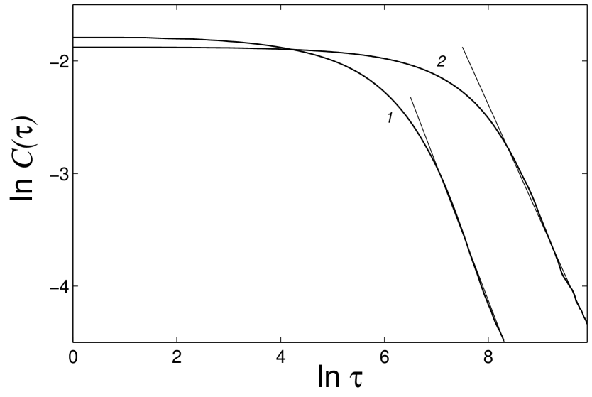
Figure 12: Power-law decrease of the autocorrelation function $C(\tau)$ in the chain with $\phi$–4 on-site potential (5), $\epsilon=1$, $T=1$ (curve 1) and $T=0.5$ (curve 2). (Double logarithmic coordinates, $\ln C(\tau)$ versus $\ln\tau$). The angle coefficient $\alpha$ determines the decrease rate. For $T=1$ $\alpha=1.2$, for $T=0.5$ $\alpha=1.02$.

The dependence of the heat conductivity $\kappa$ on reduced temperature $\tilde{T}$ is presented at Fig. 13. For low cooperativeness ($g<0.5$) the heat conductivity approaches local minimum and afterwards local maximum at $(\tilde{T}=\tilde{T}_{1})$ and monotonously decreases to zero as $\tilde{T}\rightarrow\infty$. The relative value of the maximum decreases as the cooperativeness grows and disappears for certain critical value of $\epsilon$.

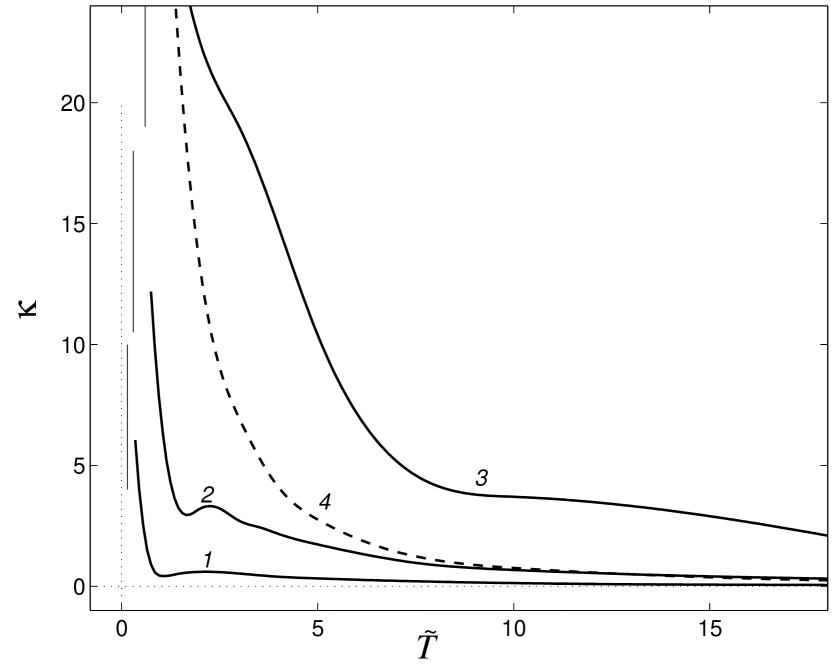
Figure 13: Heat conductivity $\kappa$ versus reduced temperature $\tilde{T}=T/\epsilon$ for the chain with double-well on-site potential (5), $\epsilon=4$ (curve 1), $\epsilon=2$ (curve 2) and $\epsilon=1$ (curve 3) and for the chain with sinh-Gordon on-site potential (6), $\omega_{0}=1$ (dashed curve 4, $\tilde{T}=T$).

In order to reveal the physical reasons of such behavior of the heat conductivity it is also reasonable to investigate the behavior of the heat capacity $c$ (Fig. 9b). As $\tilde{T}\rightarrow 0$ the heat capacity $c\rightarrow 1$. As the temperature grows, the heat capacity grows, achieves its maximum at the temperature $\tilde{T}_{c}$ and then decreases monotonously to the value less than unity. The value $\tilde{T}_{c}$ is situated near the maximum point of the heat conductivity $\tilde{T}_{1}$. Such behavior is related with the peculiarities of $\phi$–4 potential. At low temperatures the main effect is due to negative anharmonism near the ground state (therefore the heat capacity exceeds unity) and for high temperatures ($\tilde{T}\gg 1$) the process is governed by positive anharmonism bringing the heat capacity to the value below unity.

Let us now consider the frequency spectrum of vibrations of the chain. The spectrum is computed for $\epsilon=4$ $(g=1/4)$ and three characteristic temperatures $T=0.4$, 10, 100. The spectrum of the chain with harmonic on-site potential (3) does not depend on the temperature and has the form

$$E(\omega)=2\omega/\pi\sqrt{(\omega^{2}-\omega_{0}^{2})(\omega_{1}^{2}-\omega^{2})},$$ (17)

where maximum frequency $\omega_{1}^{2}=4+\omega_{0}^{2}$. For $\epsilon=4$, $\omega_{0}=4/\pi\sqrt{\epsilon}=2.546$, $\omega_{1}=3.238$. As it is demonstrated at Fig. 14a, for temperature $T=0.4$ the spectrum of the chain with on-site $\phi$–4 potential nearly coincides with the spectrum of purely harmonic chain (17). Such spectrum means that at low temperatures only thermalized phonons contribute to the frequency spectrum and other excitations do not play any significant role. For $T=10>\epsilon$ the distribution crosses the lower boundary of the propagation zone $\omega_{0}$ (Fig. 14b). Such low-frequency component may be associated with intrinsic vibrations of the solitons superlattice. For even higher temperatures $T=100\gg\epsilon$ the spectrum crosses also the upper boundary of the propagation zone $\omega_{1}$ (Fig. 14c). Such effect may be attributed only to thermalization of high-frequency discrete breathers.

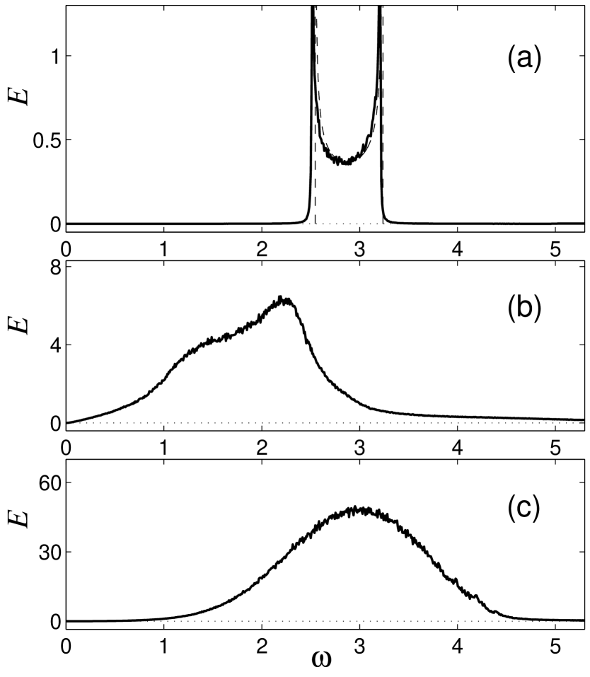
Figure 14: Frequency spectrum of energy of vibrations in the chain with double-well on-site potential (5) at temperatures $T=0.4$ (a), $T=10$ (b) and $T=100$ (c). $\epsilon=4$. Dashed line denotes the spectrum of harmonic chain (3) with $\omega_{0}=4/\pi\sqrt{\epsilon}$.

Therefore, for low temperatures $\tilde{T}<\tilde{T}_{0}=0.5g$ the dynamics of the system is close to that of harmonic chain. The heat transport is governed by weakly interacting phonons and heat conductivity diverges. For higher temperatures the heat conductivity converges. In the intermediate diapason $\tilde{T}_{0}<\tilde{T}<\tilde{T}_{1}$ the effective phonon scattering mechanism exists due to the superlattice of topological solitons, and for high temperatures $\tilde{T}>\tilde{T}_{1}$ – due to high - frequency discrete breathers. Interplay of two different mechanisms of the phonon scattering explains also the dependence of the heat conductivity on the cooperativeness of the system (Fig. 13). The minimum and maximum of heat conductivity disappear with growth of the cooperativeness since the soliton mechanism of scattering becomes less effective (the soliton-phonon interaction is closer to elastic) and simultaneously the excitation of the discrete breathers becomes easier.

7 Heat conductivity of the chain with sinh-Gordon on-site
potential

Heat conductivity of this system has been investigated in paper [16] and here it is reasonable to elucidate the details related to physical mechanisms of the process. The on-site potential (6) is single-well function with positive anharmonism. The analysis of the finite sequence $\kappa(N)$, $N=10$, 20, 40, 80 160, 320, 640, demonstrates that the heat conductivity converges for high temperatures ($T>T_{0}>0$). This observation is supported by the fact that the autocorrelation function $C(\tau)$ at high temperatures for $\tau\rightarrow\infty$ decreases exponentially (Fig. 15), and for low temperatures - by power law (Fig. 16).

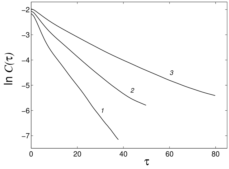
Figure 15: Exponential decrease of the autocorrelation function $C(\tau)$ in the chain with sinh-Gordon on-site potential (6), $\omega_{0}=1$, $T=10$ (curve 1), $T=7$ (curve 2) and $T=5$ (curve 3). (Semilogarythmic coordinates $\ln C(\tau)$ versus $\tau$).

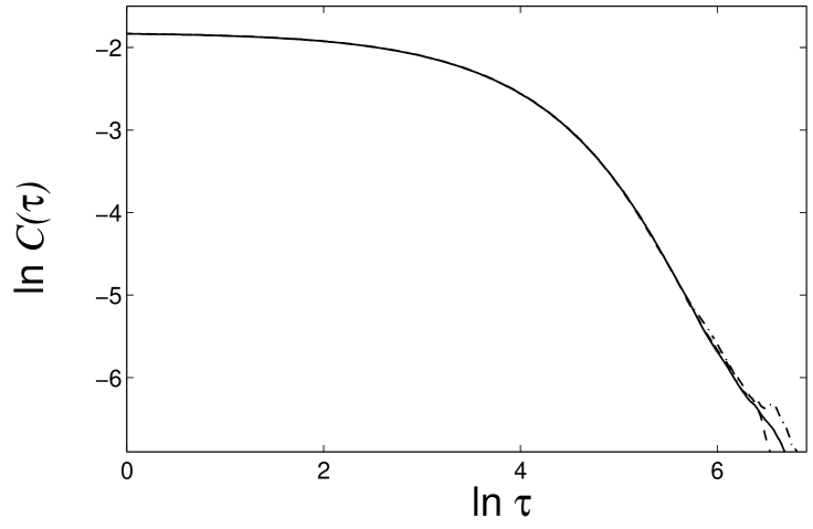
Figure 16: Power-law decrease of the autocorrelation function $C(\tau)$ in the chain with sinh-Gordon on-site potential (6), $\omega_{0}=1$, $T=2$. Solid line corresponds to the number of particles $N=500$, dotted – to $N=1000$, dashed-dotted – to $N=2000$.

The heat conductivity decreases monotonously and for $T\rightarrow\infty$ exponentially tends to zero (Fig. 13, curve 4). Positive anharmonism of the potential leads to monotonous decrease of the heat capacity (Fig. 9, curve 11). The frequency spectrum of vibrations moves towards the upper boundary of the propagation zone with growth of the temperature. These facts allow concluding that the high-frequency discrete breathers provide effective phonon scattering in this model and facilitate the convergence of the heat conductivity. Growing concentration of these breathers with the growth of the temperature leads to monotonous decrease of the heat conductivity coefficient.

Chain with on-site potential

$$V(u)=\beta u^{4}/4$$ (18)

( positive $\phi^{4}$ model) also has finite heat conductivity [17, 18]. Potential (18) as well as sinh-Gordon on - site potential (6) is single - well symmetric function with positive anharmonism. Therefore the mechanism of the phonon scattering is also related to the discrete breathers and $\kappa(T)\searrow 0$ for $T\rightarrow\infty$. For $\beta=2$ the heat conductivity $\kappa(T)\sim T^{-1.35}$ [18].

8 Conclusion

The investigation presented above demonstrates that the anharmonicity of the on-site potential does not constitute sufficient condition for the convergence of the heat conductivity coefficient. The behavior of any concrete model in the above respect depends on its peculiar nonlinear excitations which determine the process of the heat transfer and phonon scattering. Two typical mechanisms of the phonon scattering were revealed in the paper – thermalized soliton superlattice (discrete sin-Gordon and $\phi$–4 models) and discrete high-frequency breathers ($\phi$–4 and sinh-Gordon models). Phonon scattering mechanism may switch with the change of the temperature ($\phi$–4 – model).

For the discrete Frenkel-Kontorova model the zone of the converging heat conductivity for given chain length is limited by low and high temperatures and by high cooperativeness. The numerical possibilities available up to date does not allow establishing unambiguously the character of the heat conductivity outside the zone designated at Fig. 7. Still there is a reason to suggest that infinite chain for certain parameters has diverging heat conductivity, although the zone corresponding to finite heat conductivity will be larger that computed above.

Unlike Frenkel-Kontorova model, for $\phi$–4 model it is possible to demonstrate that for low temperatures the boundary of the transition to abnormal heat conduction may be achieved. It is possible to suppose that there exist a transition from infinite to finite heat conductivity with growth of temperature for any cooperativeness. The probable reason for the divergence to be detectable is the presence of odd-power terms in the on-site potential in the vicinity of the extrema of the potential wells.

The sinh-Gordon model does not allow to detect the divergence of the heat conductivity in current experiment; still, the transition also may be suggested for any cooperativeness.

It is possible to suggest that for any analytic on-site potential for low temperatures the heat conductivity will diverge.

The authors are grateful to Russian foundation of Basic Research (grant 01-03-33122), to RAS Commission for Support of Young Scientists (6th competition, grant no. 123) and to Fund for Support of Young Scientists for financial support.

A.V. Savin is grateful to International Association of Assistance for the promotion of co-operation with scientists from the New Independent States of the former Soviet Union (project INTAS no. 96-158) for financial support.

9 Appendix

9.1 Numeric realization of the Langevin thermostat

System of equations describing the dynamics of the chain attached to thermostats (7) has been integrated numerically by standard fouth-order Runge-Kutta method with constant step of integration $\Delta\tau$. Numeric realization of delta-function is performed as $\delta(\tau)=0$ for $|\tau|>\Delta\tau/2$ and $\delta(\tau)=1/\Delta\tau$ for $|\tau|\leq\Delta\tau$, i.e. the step of integration corresponds to the correlation time of the random forces. That is why in order to get correct description of the Langevin thermostat we must guarantee that the relaxation time $\tau_{r}\gg\Delta\tau$. In order to fulfill this condition the relaxation time was chosen as $\tau_{r}=10$, and the step of integration for different values of $N$, was chosen as $\Delta=0.05$, 0.025, 0.0125.

For every step of integration the random forces $\xi_{n}^{\pm}$ were taken to be constant. They were computed as independent realizations of the random value $\xi$, normally distributed with zero average $\langle\xi\rangle=0$ and dispersion $\langle\xi^{2}\rangle=2T_{\pm}/\tau_{r}\Delta\tau$. For generating the random value $\xi$ program package ZUFALL [29] was used.

The initial state for the integration of equations (7) was chosen to be equal to ground state of the chain:

$$u_{n}=u_{0},~{}~{}{u_{n}}^{\prime}=0,~{}~{}n=1,2,....,N_{+}+N+N_{-},$$ (19)

where $u_{0}=0$ for on-site potentials (3), (6) and $u_{0}=\pi$ for potentials (4), (5). It is convenient to control the accuracy of the simulation through behavior of sequence of average local heat fluxes $\{J_{n}\}_{n=N_{+}+1}^{N_{+}+N}$. If the choice of the integration step $\Delta\tau$ is correct then this sequence should be constant. If the local average heat flux changes from particle to particle then the integration step should be reduced. For growing chain length $N$ the step of integration should be also reduced in order to provide sufficient accuracy; the averaging time also grows (see [30]) and therefore the time of simulation necessary for obtaining reliable results for large $N$ turns out to be extremely large.

9.2 Computation of the correlation function

In order to compute the autocorrelation function of the heat flux $C_{N}(\tau)$ dynamics of cyclic $N$-particle chain was simulated. The thermalized chain with temperature $T$ was obtained by integrating Langevin system of equations

$$u^{\prime\prime}_{n} = u_{n+1}-2u_{n}+u_{n-1}-F(u_{n})-\gamma u^{\prime}_{n}+\xi_{n},$$

$$n=1,2,...,N~{},$$

where $n+1=1$ for $n=N$ and $n-1=N$ for $n=1$, $\gamma=0.1$ (relaxation time $\tau_{r}=10$), $\xi_{n}$ – white Gaussian noise normalized as

$$\langle\xi_{n}(\tau)\rangle=0,~{}~{}~{}\langle\xi_{n}(\tau_{1})\xi_{k}(\tau_{2})\rangle=2\gamma T\delta_{nk}\delta(\tau_{2}-\tau_{1}).$$

System (9.2) has been integrated numerically with initial conditions corresponding to the ground state of the chain. After time $\tau=10\tau_{r}$ the chain approached equilibrium with the thermostat and the coordinates

$$\{u_{n}(\tau),{u_{n}}^{\prime}(\tau)\}_{n=1}^{N}$$ (21)

corresponding to the thermalized state at temperature $T$.

Afterwards the dynamics of isolated thermalized chain was simulated. For this sake system (9.2) was integrated with zero damping $\gamma=0$ and zero external force $\xi_{n}\equiv 0$). Thermalized state (21) was used as initial condition. The result was the dependence of the general heat flux J on time $\tau$. Afterwards with the help of (16) the autocorrelation function $C_{N}(\tau)$ was computed for given thermalized state of the chain. The autocorrelation function depends significantly on concrete realization of the thermalized chain. That is why in order to improve the accuracy this procedure was performed $10^{3}\div 10^{4}$ with independent initial realizations of the thermalized state. Finally the shape of the correlation function was computed as average over all these realizations. It is worth while mentioning that the alternative way of computation (performing of one very large simulation) would not bring about any sufficient gain in the accuracy because of growing integration errors.

In order to verify the independence of the correlation function on the chain length the appropriate calculations were performed for different values of $N$. Fig. 16 demonstrates the function $C_{N}(\tau)$ for the chain with sinh-Gordon on-site potential for $\omega_{0}=1$, $T=2$ and $N=500$, 1000, 2000. It is clear that the autocorrelation function is nearly independent on $N$ (the differences are noticeable only for large times and are reduced as the number of realizations used for averaging grows). For given set of parameters $N=1000$ provides sufficient accuracy.

9.3 Comparison of Langevin and Nose-Hoover thermostats

Unlikely the Langevin thermostat, the Nose-Hoover thermostat (NHT)[24] is not stochastic. Its dynamics is completely determined by the initial conditions. It turned out to be good choice for simulations of FPU system [2, 3] but its deterministic nature can bring about artifacts in the behavior of the system. We compare this thermostat with the Langevin thermostat (LT) we use for the case of Frenkel - Kontorova model.

Let us consider the chain with fixed ends ($1<n<N+N_{+}+N_{-}$) with $N_{\pm}$ particles attached to NHT having the temperature $T_{\pm}$. Dynamics of the system is described by equations

$$u^{\prime\prime}_{n} = u_{n+1}-2u_{n}+u_{n-1}-F(u_{n})-\eta_{+}u^{\prime}_{n},$$

$$n = 2,...,N_{+},$$

$${\eta_{+}}^{\prime} = \frac{1}{\tau_{r}^{2}}\left(\frac{1}{(N_{+}-1)T_{+}}\sum_{n=2}^{N_{+}}{u_{n}^{\prime}}^{2}-1\right)$$

$$u^{\prime\prime}_{n} = u_{n+1}-2u_{n}+u_{n-1}-F(u_{n}),$$ (22)

$$n = N_{+}+1,...,N_{+}+N,$$

$$u^{\prime\prime}_{n} = u_{n+1}-2u_{n}+u_{n-1}-F(u_{n})-\eta_{-}u^{\prime}_{n},$$

$$n = N_{+}+N+1,...,N_{+}+N+N_{-}-1,$$

$${\eta_{-}}^{\prime} = \frac{1}{\tau_{r}^{2}}\left(\frac{1}{(N_{-}-1)T_{-}}\sum_{n=N_{+}+N+1}^{N_{+}+N+N_{-}}{u_{n}^{\prime}}^{2}-1\right)$$

where $F(u)=dU(u)/du$, and $\tau_{r}$ is the relaxation time of the thermostat.

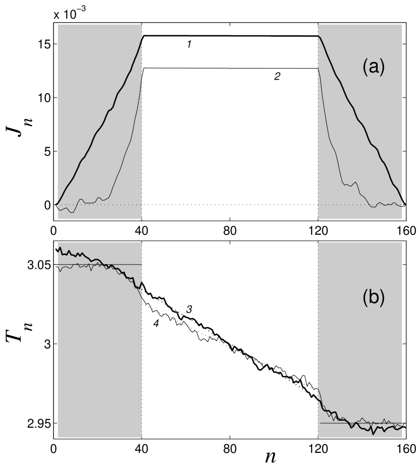
Figure 17: Distribution of local heat flux $J_{n}$ (a) and and local temperature $T_{n}$ (b) in the chain with periodic on-site potential (4), $\epsilon=1$, $N=160$, $N_{\pm}=40$, $T_{+}=3.05$, $T_{-}=2.95$, averaging time $\tau=10^{7}$. Grey zones denote the chain fragments embedded in the thermostats. Thick lines (1, 3) correspond to NHT ($\tau_{r}=1$), and thin (2, 4) – to LT ($\tau_{r}=10$).

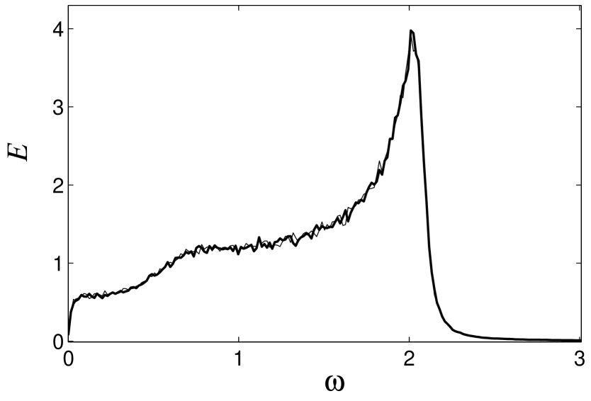
Figure 18: Frequency distribution of the energy of particle having number $N/2$ in the chain with periodic on-site potential (4), $\epsilon=1$, $N=160$, $N_{\pm}=40$, $T_{+}=3.05$, $T_{-}=2.95$. Thick line corresponds to use of NHT ($\tau_{r}=1$), and thin – to use of LT ($\tau_{r}=10$).

Usually the simulations of the heat conductivity [2, 3, 15, 17] take $\tau_{r}=1$, and $N_{+}=N_{-}=2$ (only end particles are attached to the thermostat $n=2$ and $n=N_{+}+N+N_{-}-1$). But, as stated in [25], such thermostats are not enough random – they cover only a part of the phase space and correspond to strange attractors. In order to reduce this effect we attach to the thermostat $N_{+}=N_{-}=40$ particles from every side of the chain.

The dynamics of system (22) is also completely deterministic. It should be mentioned that it is impossible to use the initial condition (19) corresponding to ground state of the system (it is stationary point of system (22)). We take the initial condition

$$u_{n}=u_{0},~{}~{}~{}{u_{n}}^{\prime}(0)=4(\xi_{n}-\frac{1}{2})\sqrt{(T_{+}+T_{-})/2},$$ (23)

where $\xi_{n}$ – independent realizations of the random variable over the interval [0,1].

We choose $\epsilon=1$ ($g=1$), $T_{+}=3.05$, $T_{-}=2.95$, $N=80$ and integrate system (22) numerically with initial condition (23). The distribution of heat fluxes $J_{n}$ and local temperatures $T_{n}$ is presented at Fig. 17 (for the sake of comparison we present also the results received bu using LT - thin lines). Within the left thermostat the heat flux grows linearly and within the other thermostat it decreases linearly with $n$. At central part of the chain the value of the heat flux does not depend on $n$. Linear temperature profile is formed and the heat conductivity coefficient may be computed according to (12) – $\kappa(N)=18.4$. Use of LT gives $\kappa(N)=18.5$ (see above), i.e. the value of $\kappa$ does not depend on the type of the thermostat.

In addition, it is possible to conclude from Fig. 18 that the frequency distribution of the energy of vibrations also does not depend on the type of thermostat used. It means that for the case of the temperatures close to the value of the potential barrier the choices of NHT or LT bring about equivalent results

The situation is strikingly different if the temperature is lower and the chain is closer to the linear case. The Nose-Hoover thermostat is not effective in this case. In order to illustrate this fact we use the model of harmonic chain. As it is clear from Fig. 3 NHT gives values of the heat flow substantially different from the correct values; at the same times the use of LT secures much better results. That is why in the present paper we used more complicated and consuming LT.

It should be mentioned that sometimes due to its simplicity NHT is used incorporate with LT [31] (LT is used for the parameters of the model where NHT is not acceptable).

References

- [1] E. Fermi, J. Pasta, and S. Ulam, Los Alamos Rpt LA-1940, 1955.
- [2] S. Lepri, L. Roberto, and A. Politi, Phys. Rev. Lett. 78, 1896 (1997).
- [3] S. Lepri, R. Livi, and A. Politi, Physica D 119, 140 (1998).
- [4] S. Lepri, R. Livi, and A. Politi, Evrophys. Lett. 43, 271 (1998).
- [5] R. Rubin and W. Greer, J. Math. Phys. (N.Y.) 12, 1686 (1971).
- [6] A. Casher and J.L. Lebowitz, J. Math. Phys. (N.Y.) 12, 1701 (1971).
- [7] A. Dhar, Phys. Rev. Lett. 86, 5882 (2001).
- [8] A. Dhar, Phys. Rev. Lett. 86, 3554 (2001).
- [9] A.V. Savin, G.P. Tsironis, and A.V. Zolotaryuk, Phys. Rev. Lett. 88, (15)/154301 (2002).
- [10] G. Casati and T. Prosen, arXiv:cond-mat/0203331.
- [11] T. Hatano, Phys. Rev. E 59, R1 (1999).
- [12] G. Casati, J. Ford, F. Vivaldi, and V.M. Visscher, Phys. Rev. Lett. 52, 1861 (1984).
- [13] T. Prosen, M. Robnik, J. Phys. A 25, 3449 (1992).
- [14] M. J. Gillan, R. W. Holloway, J. Phys. C 18, 5705 (1985).
- [15] B. Hu, B. Li, and H. Zhao, Phys. Rev. E 57, 2992 (1998).
- [16] G.P. Tsironis, A.R. Bishop, A.V. Savin, and A.V. Zolotaryuk, Phys. Rev. E 60, 6610 (1999).
- [17] B. Hu, B. Li, and H. Zhao, Phys. Rev. E 61, 3828 (2000).
- [18] K. Aoki and D. Kuznezov, Phys. Lett. A 265, 250 (2000); arXiv:chao-dyn/9910015.
- [19] F. Bonetto, J.L. Lebowitz and L. Ray-Bellet in Mathematical Physics 2000, ed. A. Fokas, A. Grigoryan, T. Kibble and B. Zegarlins
- [20] S. Lepri, R. Livi, and A. Politi, arXiv:cond-mat/0112193.
- [21] C. Giardina, R. Livi, A. Politi, and M. Vassalli, Phys. Rev. Lett. 84 2144 (2000).
- [22] O.V. Gendelman and A.V. Savin, Phys. Rev. Lett. 84, 2381 (2000).
- [23] A.V. Savin and O.V. Gendelman, Fizika Tverdogo Tela 43, 341 (2001) [Physics of the Solid State 43, 355 (2001)].
- [24] S. Nose, J. Chem. Phys. 81, 511 (1984); W. G. Hoover, Phys. Rev. A 31, 1695 (1985).
- [25] A. Fillipov, B. Hu, B. Li, and A. Zeltser, J. Phys. A 31, 7719, (1998).
- [26] K. Aoki and D. Kusnezov, Phys. Rev. Lett. 86, 4029 (2001).
- [27] R. Kubo, M. Toda, and N. Hashitsume, Statistical Physics II, Springer Ser. Solid State Sci., 31 (1991).
- [28] V.L. Pokrovsky, A.L. Talapov, Zh. Eksp. Teor. Fiz. 75, 1151 (1978).
- [29] W.P. Petersen, ”Lagged Fibonacci Random Number Generators for the NEC SX-3” is to be published in the International Journal of High Speed Computing (1994); ftp://ftp.netlib.org/random/zufall.f
- [30] A. Dhar, Phys. Rev. Lett. 87, 069401 (2001).
- [31] M. Terraneo, M. Peyrard, and G. Casati, Phys. Rev. Lett. 88, 094302 (2002).