Langevin dynamics of the Coulomb frustrated ferromagnet: a mode-coupling analysis.

Abstract

We study the Langevin dynamics of the soft-spin, continuum version of the Coulomb frustrated Ising ferromagnet. By using the dynamical mode-coupling approximation, supplemented by reasonable approximations for describing the equilibrium static correlation function, and the somewhat improved dynamical self-consistent screening approximation, we find that the system displays a transition from an ergodic to a non-ergodic behavior. This transition is similar to that obtained in the idealized mode-coupling theory of glassforming liquids and in the mean-field generalized spin glasses with one-step replica symmetry breaking. The significance of this result and the relation to the appearance of a complex free-energy landscape are also discussed.

I Introduction

Models with a competition between a short-range ordering interaction and a long-range frustrating interaction have been recently introduced to explain the slowing down of relaxation in supercooled liquids and the resulting glass transitionKKZNT95 . The underlying picture is as follows: any given liquid possesses a locally preferred structure which is different than that of the actual crystalline phase, and this local arrangement of the molecules in the liquid cannot propagate at long distances to tile the whole space and form an “ideal crystal” because of ubiquitous frustration. It has been arguedKKZNT95 that, for weak enough frustration, this phenomenon can be described via effective interactions acting on very different length scales: a short-range term describing the tendency to extend the locally preferred structure and a long-range, Coulomb-like term describing the frustration-induced free-energy cost associated with this spatial extension. Such Coulomb frustrated systems have been shown, both by scaling argumentsKKZNT95 ; VTK00 and by Monte Carlo simulationGrTV01 , to display the generic features observed in fragile glassforming liquids, most notably the super-Arrhenius temperature dependence of the relaxation time and the two-step, non-exponential decay of the correlation function.

These Coulomb frustrated models have also been used in quite different contexts to describe the formation of modulated spatial patterns on mesoscopic length scales, such as lamellar and cubic phases in diblock copolymer meltsOK86 ; L80 ; FH87 , microemulsions in water-oil-surfactant mixturesS83 ; WCS92 , or stripe phases in high temperature superconductorsEK93 . In all these cases, slow relaxation is usually observed, and it has been recently arguedScWo00 that high-temperature superconductors could indeed form a “stripe glass” in which glassiness is self generated, i.e., does not result from the presence of quenched disorder. This latter result has been obtained through an investigation of the properties of the free-energy landscape of the Coulomb frustrated $\phi^{4}$ scalar field theory: by using a thermodynamic approach combining the replica method proposed for the study of structural glassesM95 ; MP99 and a particular approximation, the self-consistent screening approximation (SCSA)AJBa74 , for calculating the pair correlation functions, Schmalian and WolynesScWo00 have derived that the free-energy landscape of the Coulomb frustrated model becomes non-trivial below some temperature $T_{A}$ at which an exponentially large number of metastable states appears; the associated configurational entropy decreases with further decrease of the temperature and vanishes at a lower temperature $T_{K}$ScWo00 ; SW201 ; endnote1 .

Motivated by these results giving evidence for fragile glassforming behavior in Coulomb frustrated models, we have studied the Langevin dynamics of the Coulomb frustrated $\phi^{4}$ scalar field theory within the mode-coupling and related approximations. Mode-coupling approaches have been widely used to study glassforming liquidsgotze91 ; Cummins99 , and the dynamical ergodicity-breaking singularity predicted to occur in the weakly supercooled liquid regions, albeit “avoided” in real systems, is taken by many as a canonical feature of fragile glassforming systems. It is therefore tempting to investigate whether Coulomb frustrated models also display this feature.

The paper is organized as follows. We first present the model and summarize the equilibrium phase behavior and the results previously obtained by Schmalian and Wolynes. We also introduce the Langevin equation describing the relaxational dynamics of the system. In section III, we derive the evolution equations followed by the equilibrium time-dependent correlation function obtained within two resummation schemes of perturbative expansions: the mode-coupling approximation and the dynamical SCSA. Section IV is devoted to the search for an ergodicity-breaking transition. We find that such a phenomenon is indeed observed with the two approximations considered. We also show that the dynamical singularity predicted by the dynamical SCSA coincides with the temperature $T_{A}$ at which the replica analysis of RefsScWo00 ; SW201 predicts the occurrence of an exponentially large number of metastable states. In section V, we present the full numerical solution of the mode-coupling equations, thereby obtaining the time-evolution of the equilibrium correlation function; this latter is similar to that obtained in the idealized mode-coupling theory of supercooled liquidsgotze91 and in mean-field generalized spin-glass modelsKT87 ; BCKM96 ; CHS93 . In the last two section, we address the question of sensitivity of the results to the level and the details of the approximation scheme and we give some concluding remarks.

II Model

We consider the field-theoretical version of the $3$-dimensional Coulomb frustrated Ising ferromagnet defined by the Hamiltonian

$$H[\phi]= \frac{1}{2}\int d^{3}{\bf{x}}\left\{(\nabla\phi({\bf{x}}))^{2}+r_{0}\phi^{2}({\bf{x}})+\frac{u}{2}\phi^{4}({\bf{x}})\right\}+\frac{Q}{8\pi}\int d^{3}{\bf{x}}\int d^{3}{\bf{x}}^{\prime}\frac{\phi({\bf{x}})\phi({\bf{x^{\prime}}})}{|{\bf{x}}-{\bf{x^{\prime}}}|}$$ (1)

$$= \frac{V}{2}\int\frac{d^{3}{\bf k}}{(2\pi)^{3}}\left(r_{0}+k^{2}+\frac{Q}{k^{2}}\right)\phi_{-{\bf k}}\phi_{{\bf k}}+\frac{uV}{4}\int\frac{d^{3}{\bf k_{1}}}{(2\pi)^{3}}\int\frac{d^{3}{\bf k_{2}}}{(2\pi)^{3}}\int\frac{d^{3}{\bf k_{3}}}{(2\pi)^{3}}\phi_{{\bf k_{1}}}\phi_{{\bf k_{2}}}\phi_{{\bf k_{3}}}\phi_{-{\bf k_{1}}-{\bf k_{2}}-{\bf k_{3}}},$$ (2)

where $\phi({\bf{x}})$ is a real scalar field ($\phi_{\bf k}$, the associated ${\bf k}-$Fourier component), $V$ is the volume, $u$ is a strictly positive coupling constant, $Q$ is the frustration parameter, and all momentum integrations are performed up to a cut-off $\Lambda$, i.e., $|{\bf k}|\leq\Lambda$; $r_{0}$ is a temperature-dependent mass which is proportional to the deviation, $T-T^{0}_{c,MF}$, from the mean-field transition temperature of the unfrustrated $(Q=0)$ model.

Figure 1: Temperature ($r_{0}$)-frustration ($Q^{1/4}$) equilibrium phase diagram in the self-consistent Hartree approximation. The full line denotes the fluctuation-induced first-order transition to modulated phases; below this line, the paramagnetic phase exists in a metastable state. The coupling constant $u$ is set equal to $1$.

The equilibrium partition function is

$$Z=\int{\cal D}\phi e^{-H(\phi)/T}.$$ (3)

In what follows, we take $\Lambda=1$, and $T$ is set equal to $1$ in Eq. (3) so that the whole temperature dependence is contained in $r_{0}$. We are interested in the weak-frustration region for which $Q<<1$.

In the absence of frustration $(Q=0)$, the model defined by Eqs. (1-3) reduces to the usual $\phi^{4}$ theory. It undergoes a second-order transition at a finite temperature $T^{0}_{c}$ to a broken-symmetry phase characterized by a non-zero value of $<\phi_{{\bf k=0}}>$, where $<>$ denotes an equilibrium average. For $Q>0$, an ordered phase with $<\phi_{{\bf k=0}}>\neq 0$ is forbidden, but the system can still undergo a phase transition at a temperature $T_{DO}(Q)$ to a phase with long-range modulated order. This transition has been studied by Monte Carlo simulation for the case of the Coulomb frustrated Ising ferromagnet on a cubic latticeGTV01b and via the self-consistent Hartree approximation for a Hamiltonian similar to Eq. (1) describing microphase separation in diblock copolymer meltsFH87 : it has then been shown that, whereas the mean-field theory predicts a second-order transition, the fluctuations change the order of the transition and induce a first-order transition. Such a fluctuation-induced first-order transition was first discussed by Brazovskii for a related modelB75 . Within the self-consistent Hartree approximation, the equilibrium (connected) correlation function

$$VC({\bf k})=<\phi_{-{\bf k}}\phi_{{\bf k}}>-<\phi_{-{\bf k}}><\phi_{{\bf k}}>$$ (4)

is obtained via a self-consistent equation; for instance, in the paramagnetic phase where $<\phi_{{\bf k}}>=0$, this equation is

$$C^{-1}({\bf{k}})=r_{0}+k^{2}+\frac{{Q}}{k^{2}}+3u\int\frac{d^{3}{\bf q}}{(2\pi)^{3}}C({\bf{q}}).$$ (5)

The renormalized mass, $r=r_{0}+3u\int\frac{d^{3}{\bf q}}{(2\pi)^{3}}C({\bf{q}})$, is then given by

$$r=r_{0}+3u\int\frac{d^{3}{\bf q}}{(2\pi)^{3}}\frac{1}{r+q^{2}+\frac{Q}{q^{2}}}.$$ (6)

Since $k^{2}+\frac{Q}{k^{2}}$ is minimum for non-zero wave vectors with modulus $k_{m}=Q^{1/4}$, a value characterizing the incipient modulated order, one easily checks that $r$ only goes to zero when $r_{0}\to-\infty$. This means that the paramagnetic phase is (meta)stable at all finite “temperatures”, its spinodal being depressed to $r_{0}\to-\infty$. The Hartree approximation allows one to calculate the free energy of the paramagnetic phase and that of the phase with modulated order. One then obtains the temperature $r_{0}^{DO}(Q)$ of the first-order transition at the point at which the two free energies are equal. The details are given in Appendix A and the resulting phase diagram is shown in Fig. 1.

In their recent work, Schmalian and WolynesScWo00 have applied the thermodynamic approach of non-random glassforming systems developed by Mézard and ParisiMP99 to the Coulomb frustrated model. The basic idea, originally motivated by the behavior of a class of mean-field generalized spin glasses such as $p-$spin and Potts glassesKT87 ; BCKM96 , is that glassiness arises because of the occurrence of an exponentially large number of metastable states. This occurrence, and the associated emergence of a non-zero complexity or configurational entropy, can be more conveniently studied within the replica formalismM95 . Approximations are of course necessary to solve the corresponding many-body problem and obtain all relevant correlation functions. Schmalian and Wolynes have shown that within the SCSAAJBa74 , an approximation that goes beyond the Hartree result in that it explicitly includes more diagrams of the perturbative expansionendnote2 , there is a temperature $T_{A}$ at which an exponentially large number of metastable states emerges, as signaled by a non-zero configurational entropy. The configurational entropy decreases with further decay of the temperature and it vanishes at a temperature $T_{K}$ at which the system undergoes a random first-order transition to an “ideal glass”ScWo00 .

In the present work, we focus on the dynamics of the Coulomb frustrated model defined by Eq. (1). The starting point is the Langevin equation,

$$\frac{\partial\phi_{{\bf{k}}}(t)}{\partial t}=-\frac{{\delta}(H[\phi_{{\bf{k}}}(t)]/V)}{\delta\phi_{-{\bf{k}}}(t)}+\eta_{{\bf{k}}}(t),$$ (7)

that describes the purely relaxational dynamics of the system; $\eta_{{\bf{k}}}(t)$ is a gaussian thermal noise with $<\eta_{{\bf{k}}}(t)>=0$ and $<\eta_{{\bf{k}}}(t)\eta_{{\bf{k}}^{\prime}}(t^{\prime})>=2T\delta({\bf{k}}+{\bf{k}}^{\prime})\delta(t-t^{\prime})$. Eq. (7) can be explicitly written as

$$\frac{\partial\phi_{{\bf{k}}}(t)}{\partial t} =-(r_{0}+k^{2}+\frac{{Q}}{k^{2}})\phi_{{\bf{k}}}$$

$$- u\int\frac{d^{3}{\bf{k}}_{1}}{(2\pi)^{3}}\int\frac{d^{3}{\bf{k}}_{2}}{(2\pi)^{3}}\phi_{{\bf{k}}_{1}}\phi_{{\bf{k}}_{2}}\phi_{{\bf{k}}-{{\bf{k}}_{1}}-{{\bf{k}}_{2}}}+\eta_{{\bf{k}}}(t).$$ (8)

Solving this set of coupled non-linear dynamical equations is a daunting task, and virtually all available approximations amount to performing some self-consistent resummation of perturbative expansions, e.g,. expansions in powers of the coupling constant $u$ or of the inverse of the number of components of the field, $1/n$, for an $O(n)$ model. In what follows, we shall consider two such self-consistent resummation schemes, the mode-coupling approximation and the dynamical SCSAendnote3 .

III Dynamical self-consistent approximations

To introduce the mode-coupling approximation, we first define the time-dependent correlation function $C({\bf k},t,t^{\prime})$ and the associated response function $G({\bf k},t,t^{\prime})$:

$$\delta({\bf{k}}+{\bf{k}}^{\prime})C({\bf{k}},t,t^{\prime}) = <\phi_{{\bf{k}}}(t)\phi_{{\bf{k}}^{\prime}}(t^{\prime})>,$$ (9)

$$\delta({\bf{k}}+{\bf{k}}^{\prime})G({\bf{k}},t,t^{\prime}) = <\frac{\partial\phi_{{\bf{k}}}(t)}{\partial\eta_{{\bf{k}}^{\prime}}(t^{\prime})}>$$ (10)

$$= \frac{1}{2T}<\phi_{{\bf{k}}}(t)\eta_{{\bf{k}}^{\prime}}(t^{\prime})>.$$

As in the preceding section, we set $T=1$ in the following.

The perturbative expansion of $C({\bf k},t,t^{\prime})$ and $G({\bf k},t,t^{\prime})$ in powers of $u$ is more conveniently expressed by introducing the zeroth-order correlation and response functions,

$$C_{0}({\bf{k}},t,t^{\prime})= \frac{1}{\mu({\bf{k}})}\exp\left[\mu({\bf{k}})(t-t^{\prime})\right],$$ (11)

$$G_{0}({\bf{k}},t,t^{\prime})= \exp\left[\mu({\bf{k}})(t-t^{\prime})\right],$$ (12)

where

$$\mu({\bf{k}})=r_{0}+k^{2}+\frac{{{Q}}}{k^{2}},$$ (13)

and the two kernels $\Sigma({\bf{k}},t,t^{\prime})$ and $D({\bf{k}},t,t^{\prime})$ defined though the standard Dyson equations,

$$C({\bf{k}},t,t^{\prime}) = \int_{0}^{t}dt_{1}\int_{0}^{t^{\prime}}dt_{2}G({\bf{k}},t,t_{1})\left[2\delta(t_{1}-t_{2})+D({\bf{k}},t_{1},t_{2})\right]G({\bf{k}},t^{\prime},t_{2}),$$ (14)

$$G({\bf{k}},t,t^{\prime}) = G_{0}({\bf{k}},t,t^{\prime})+\int_{t^{\prime}}^{t}dt_{1}\int_{t^{\prime}}^{t_{1}}dt_{2}G_{0}({\bf{k}},t,t_{1})\Sigma({\bf{k}},t_{1},t_{2})G({\bf{k}},t_{2},t^{\prime}).$$ (15)

The diagrammatic representation of the perturbative expansion and a detailed derivation of the mode-coupling approximation can be found in Ref.BCKM96 ; the only difference with the cases considered in BCKM96 is the presence of the frustration term $Q/k^{2}$ in the expression of $\mu(k)$, and we merely sketch here the main steps of the derivation.

The mode-coupling approximation amounts to expanding the kernels $D({\bf{k}},t,t^{\prime})$ and $\Sigma({\bf{k}},t,t^{\prime})$ to second order in $u$ and replacing the bare (zeroth-order) functions $C_{0}({\bf{k}},t,t^{\prime})$ and $G_{0}({\bf{k}},t,t^{\prime})$ that appear in the resulting expressions by their renormalized counterparts $C({\bf{k}},t,t^{\prime})$ and $G({\bf{k}},t,t^{\prime})$. This leads toBCKM96 :

$$D({\bf{k}},t,t^{\prime})\simeq 6u^{2}\int\frac{d^{3}{\bf k}_{1}}{(2\pi)^{3}}\int\frac{d^{3}{\bf k}_{2}}{(2\pi)^{3}}C({\bf{k}}_{1},t,t^{\prime})C({\bf{k}}_{2},t,t^{\prime})C({\bf k}-{\bf k}_{1}-{\bf k}_{2},t,t^{\prime}),$$ (16)

$$\Sigma({\bf{k}},t,t^{\prime})\simeq 18u^{2}\int\frac{d^{3}{\bf k}_{1}}{(2\pi)^{3}}\int\frac{d^{3}{\bf k}_{2}}{(2\pi)^{3}}C({\bf{k}}_{1},t,t^{\prime})C({\bf{k}}_{2},t,t^{\prime})G({\bf k}-{\bf k}_{1}-{\bf k}_{2},t,t^{\prime}).$$ (17)

At the same time $\mu({\bf{k}})$ is renormalized to include the so-called tadpole diagrams, which replaces Eq. (13) by an expression similar to that obtained within the static Hartree approximation.

In this work, we are interested by the dynamical properties of the system at equilibrium: therefore, the fluctuation-dissipation theorem and the time-translation invariance apply, which reduces the dependence upon the two times $t$ and $t^{\prime}$ to the mere dependence on the difference $t-t^{\prime}$ and gives

$$G({\bf{k}},t)=-\Theta(t)\frac{\partial C({\bf{k}},t)}{\partial t}$$ (18)

and

$$\Sigma({\bf{k}},t)=-\Theta(t)\frac{\partial D({\bf{k}},t)}{\partial t},$$ (19)

where $\Theta(t)$ is the Heaviside step function ($\Theta(t)$ is equal to $0$ for $t<0$ and to $1$ pour $t>0$). Applying the operator $G_{0}^{-1}({\bf k})=\left[\mu({\bf{k}})+\frac{\partial}{\partial t}\right]$ to both sides of Eq. (15) yields

$$\frac{\partial G({\bf{k}},t)}{\partial t}=\delta(t)-\mu({\bf{k}})G({\bf{k}},t)+\int_{0}^{t}dt^{\prime}\Sigma({\bf{k}},t-t^{\prime})G({\bf{k}},t^{\prime}),$$ (20)

which, when combined with the time derivative of Eq. (18),

$$\frac{\partial G({\bf{k}},t)}{\partial t}=-\delta(t)\left(\frac{\partial C({\bf{k}},t)}{\partial t}\right)_{t=0}-\Theta(t)\frac{\partial^{2}C({\bf{k}},t)}{\partial t^{2}},$$ (21)

gives

$$\left(\frac{\partial C({\bf{k}},t)}{\partial t}\right)_{t=0}=-1.$$ (22)

For $t>0$, the equation for the response function thus reads

$$\frac{\partial G({\bf{k}},t)}{\partial t}=-\mu({\bf{k}})G({\bf{k}},t)+\int_{0}^{t}dt^{\prime}\Sigma({\bf{k}},t-t^{\prime})G({\bf{k}},t^{\prime})$$ (23)

with the initial condition $G({\bf{k}},t=0^{+})=1$. By Laplace transforming Eqs. (18), (19) and (23) and using the initial condition $\left(\frac{\partial C({\bf{k}},t)}{\partial t}\right)_{t=0}=-G({\bf{k}},t=0^{+})=-1$, one finally obtains

$$1= \left(z{\hat{C}}({\bf{k}},z)+C({\bf{k}},t=0)\right)\times$$

$$\times \left(\mu({\bf{k}})-iz-z{\hat{D}}({\bf{k}},z)-D({\bf{k}},t=0)\right),$$ (24)

where $\hat{C}({\bf{k}},z)=i\int_{0}^{\infty}dte^{izt}C({\bf{k}},t)$, and a similar expression holds for ${\hat{D}}({\bf{k}},z)$. Going back to the time dependence leads to

$$\frac{\partial C({\bf{k}},t)}{\partial t}= -\left(\mu({\bf{k}})-D({\bf{k}},t=0)\right)C({\bf{k}},t)$$

$$- \int_{0}^{t}dt^{\prime}D({\bf{k}},t-t^{\prime})\frac{\partial C({\bf{k}},t^{\prime})}{\partial t^{\prime}}$$ (25)

with the initial condition $C({\bf{k}},t=0)=\left(\mu({\bf{k}})-D({\bf{k}},t=0)\right)^{-1}$ that follows from Eqs. (22) and (III).

The mode-coupling approximation finally results in the following self-consistent equation for the time-dependent correlation function at equilibrium:

$$\frac{\partial C({\bf{k}},t)}{\partial t}= -C({\bf{k}},t=0)^{-1}C({\bf{k}},t)$$

$$- \int_{0}^{t}dt^{\prime}D({\bf{k}},t-t^{\prime})\frac{\partial C({\bf{k}},t^{\prime})}{\partial t^{\prime}}$$ (26)

with

$$D({\bf{k}},t)= 6u^{2}\int\frac{d^{3}{\bf k}_{1}}{(2\pi)^{3}}\int\frac{d^{3}{\bf k}_{2}}{(2\pi)^{3}}C({\bf{k}}_{1},t)C({\bf{k}}_{2},t)\times$$

$$\times C({\bf k}-{\bf k}_{1}-{\bf k}_{2},t).$$ (27)

Except for the absence of inertial term, $\frac{\partial^{2}C({\bf{k}},t)}{\partial t^{2}}$, in the purely relaxational dynamics associated with the Langevin equation and the cubic dependence of the memory kernel $D({\bf{k}},t)$ on the correlation function $C({\bf{k}},t)$, the above equations are similar to the mode-coupling equations used to describe the time-dependent density fluctuations in supercooled liquidsgotze91 ; they are also analogous to those derived for the mean-field spin glass with $4$-spin interactionsBCKM96 ; CHS93 .

The necessary input for solving the self-consistent Eqs. (III) and (III) is the knowledge of the equilibrium static correlation function $C({\bf{k}},t=0)$. Treating the statics and the dynamics of the system on an equal footing, as for instance done in the above derivation, leads to considering a mode-coupling approximation for the static correlation function, $C({\bf{k}},t=0)=\left(\mu({\bf{k}})-D({\bf{k}},t=0)\right)^{-1}$. However, we shall rather introduce more flexibility in the mode-coupling scheme (a flexibility that goes with the many ways to implement the self-consistency at the second order of the perturbative expansion) by allowing $C({\bf{k}},t=0)$ to be computed with several approximations, such as the Hartree approximation and the SCSA, that are a priori better behaved than the mode-coupling approximation as far as the static properties are concerned.

A somewhat refined resummation scheme is provided by the dynamical SCSA. (As mentioned in endnote2 , it consists in using an $n$-component vector field $\phi$, resumming self-consistently all the diagrams of order $1/n$ in the large $n$ expansion, and, eventually, for the problem considered here, setting $n$ equal to $1$.) Details on the derivation of the approximate equation for the time-dependent correlation function $C({\bf{k}},t)$ can be found in Refs.BCKM96 ; MCJPB97 . A convenient way to proceed is to introduce a complex auxiliary field $\sigma({\bf{x}})$ such that the partition function, Eq. (3), can be rewritten $Z=\int\int{\cal D}\phi{\cal D}\sigma e^{-H[\phi,\sigma]}$ (here $T=1$) with

$$H[\phi,\sigma]= \frac{1}{2}\int d^{3}{\bf{x}}\left\{(\nabla\phi({\bf{x}}))^{2}+r_{0}\phi^{2}({\bf{x}})-\sigma^{2}({\bf{x}})\right.$$

$$+ \left.\sqrt{2u}\sigma({\bf{x}})\phi^{2}({\bf{x}})\right\}$$

$$+ \frac{Q}{8\pi}\int d^{3}{\bf{x}}\int d^{3}{\bf{x}}^{\prime}\frac{\phi({\bf{x}})\phi({\bf{x^{\prime}}})}{|{\bf{x}}-{\bf{x^{\prime}}}|}.$$ (28)

The field $\sigma({\bf{x}})$ is such that $<\sigma({\bf{x}})>=\sqrt{u/2}<\phi^{2}({\bf{x}})>$ and its connected pair correlation function $C_{\sigma}({\bf{x}},{\bf{x}}^{\prime})=<\sigma({\bf{x}})\sigma({\bf{x}}^{\prime})>_{c}$ is equal to

$$C_{\sigma}({\bf{x}},{\bf{x}}^{\prime})= -\delta({\bf{x}}-{\bf{x}}^{\prime})$$

$$+ u/2(<\phi^{2}({\bf{x}})\phi^{2}({\bf{x}}^{\prime})>-<\phi^{2}({\bf{x}})><\phi^{2}({\bf{x}}^{\prime})>).$$ (29)

One can then apply to the dynamics of the coupled fields $\sigma({\bf{x}})$ and $\phi({\bf{x}})$ a treatment similar to that sketched above. Defining the equilibrium time-dependent correlation function $C_{\sigma}({\bf k},t)$ via $\delta({\bf{k}}+{\bf{k}}^{\prime})C_{\sigma}({\bf{k}},t)=<\sigma_{{\bf{k}}}(t)\sigma_{{\bf{k}}^{\prime}}(0)>_{c}$, the associated kernel $D_{\sigma}({\bf{k}},t)$ obtained through the Dyson equation (see above), and similar functions for the response properties, one can perform a mode-coupling approximation to the coupled dynamical equations for the fields $\sigma({\bf{x}})$ and $\phi({\bf{x}})$. This leads to Eq. (III) with $D({\bf{k}},t)$ now given byMCJPB97

$$D({\bf{k}},t)=2u\int\frac{d^{3}{\bf p}}{(2\pi)^{3}}C_{\sigma}({\bf p},t)C({\bf k}-{\bf p},t);$$ (30)

the auxiliary-field correlation function $C_{\sigma}({\bf{k}},t)$ is solution of the equation

$$\frac{\partial C_{\sigma}({\bf{k}},t)}{\partial t}= C_{\sigma}({\bf{k}},t=0)^{-1}C_{\sigma}({\bf{k}},t)$$

$$- \int_{0}^{t}dt^{\prime}D_{\sigma}({\bf{k}},t-t^{\prime})\frac{\partial C_{\sigma}({\bf{k}},t^{\prime})}{\partial t^{\prime}}$$ (31)

with

$$D_{\sigma}({\bf{k}},t)=-u\int\frac{d^{3}{\bf q}}{(2\pi)^{3}}C({\bf q},t)C({\bf k}-{\bf q},t).$$ (32)

These equations are supplemented by the initial conditions $C({\bf k},t=0)=\left(\mu({\bf{k}})-D({\bf{k}},t=0)\right)^{-1}$ and $C_{\sigma}({\bf k},t=0)=-\left(1-D_{\sigma}({\bf{k}},t=0)\right)^{-1}$ which are easily shown to be identical to the equilibrium, static SCSA equations first derived by BrayAJBa74 .

IV Transition from ergodic to non-ergodic behavior

It is well known that mode-coupling and related approximations, when applied to glassforming systems, may lead to a dynamical singularitygotze91 ; BCKM96 . This latter corresponds to a transition from an ergodic to a non-ergodic behavior and is not associated with any thermodynamic equilibrium transition. For searching for such a singularity in the above equations, it is convenient to Laplace transform Eq. (III), which gives

$$\hat{C}({\bf{k}},z)=\frac{-C({\bf{k}},t=0)}{z-\displaystyle\frac{1}{C({\bf{k}},t=0)(i+\hat{D}({\bf{k}},z))}}.$$ (33)

An ergodicity-breaking transition is associated with the appearance of a non-zero value of the long-time limit of the correlation function, $C({\bf{k}},t\to\infty)$; as a result, in the small-$z$ limit, $\hat{C}({\bf{k}},z)\sim-\frac{C({\bf{k}},t\to\infty)}{z}$ and $\hat{D}({\bf{k}},z)\sim-\frac{D({\bf{k}},t\to\infty)}{z}$, which when inserted in Eq. (33) leads to

$$D({\bf{k}},t\to\infty)=\frac{C({\bf{k}},t\to\infty)}{C({\bf{k}},t=0)(C({\bf{k}},t=0)-C({\bf{k}},t\to\infty))}.$$ (34)

The kernel $D({\bf{k}},t\to\infty)$ is obtained from Eq. (III) for the mode-coupling approximation and from Eqs. (30)-(32) for the dynamical SCSA.

Consider first the equation resulting from the mode-coupling approximation,

$$\frac{C({\bf{k}},t\to\infty)}{C({\bf{k}},t=0)-C({\bf{k}},t\to\infty)}=6u^{2}C({\bf{k}},t=0)\int\frac{d^{3}{\bf k}_{1}}{(2\pi)^{3}}\int\frac{d^{3}{\bf k}_{2}}{(2\pi)^{3}}C({\bf{k}}_{1},t\to\infty)C({\bf{k}}_{2},t\to\infty)C({\bf k}-{\bf k}_{1}-{\bf k}_{2},t\to\infty).$$ (35)

Note that this actually represents a set of coupled equations for the various ${\bf k}$-modes. The necessary input for solving this equation is the knowledge of the equilibrium static correlation function $C({\bf{k}},t=0)$ (see discussion above). We consider here two standard approximations:

(i) the Hartree approximation, already presented in Eqs. (5) and (6), and

(ii) the SCSA, described in the previous section and leading to

$$C^{-1}({\bf{k}},0)=\mu({\bf{k}})+2u\int\frac{d^{3}{\bf{q}}}{(2\pi)^{3}}\frac{C({\bf{k}}-{\bf{q}},0)}{1+u\Pi({\bf{q}})}.$$ (36)

where

$$\mu({\bf{k}})=r_{0}+k^{2}+\frac{{Q}}{k^{2}}+u\int\frac{d^{3}{\bf q}}{(2\pi)^{3}}C({\bf{q}},0)$$ (37)

and

$$\Pi({\bf{k}})=\int\frac{d^{3}{\bf q}}{(2\pi)^{3}}C({\bf{q}},0)C({\bf{k}}-{\bf{q}},0).$$ (38)

Note that if one neglects the term $u\Pi({\bf{q}})$ in Eq. (36), one recovers the Hartree approximation.

In both cases, only the paramagnetic phase $<\phi_{\bf k}>=0$, is considered. From now on, we take $u=1$ (recall that all momentum integrations are cut-off at $\Lambda=1$).

Other approximations will be discussed in section VI.

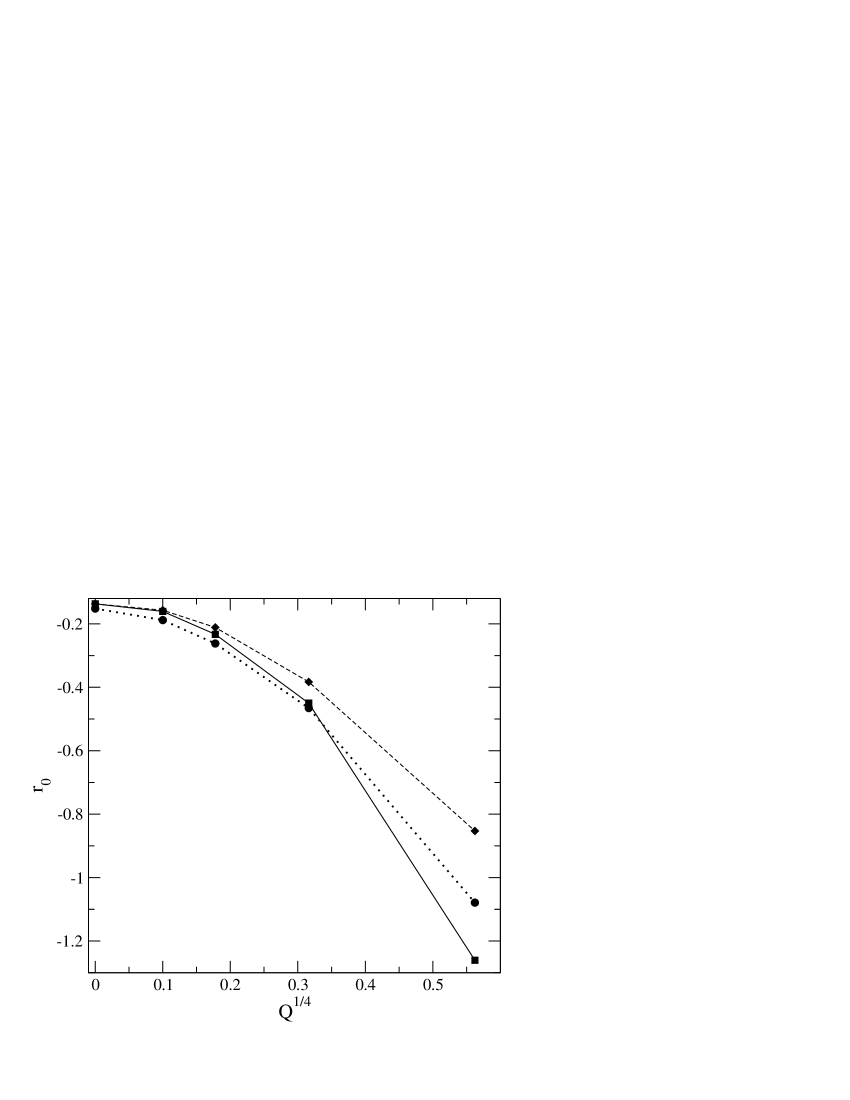
Figure 2: Ergodicity-breaking transition in the $r_{0}-(Q^{1/4})$ diagram. Dotted line: mode-coupling approximation with the static Hartree approximation; dashed line: mode-coupling approximation with the static SCSA; full line: dynamical SCSA.

We have solved the set of coupled equations, Eq. (35), by an iterative method. We find that with the above two approximations, the mode-coupling approach does lead to an ergodicity-breaking transition for the Coulomb frustrated model. When decreasing the temperature, i.e., the bare mass $r_{0}$, one reaches a point at which $C({\bf k},t\to\infty)$ discontinuously jumps to a non-zero value. The transition temperature increases as frustration decreases; it seems to reach continuously, when $Q\to 0$, the (equilibrium) critical temperature of the unfrustrated system, i.e., of the standard $\phi^{4}$ theory in either the Hartree approximation or the SCSA. This behavior is illustrated in Fig. 2. One observes a discrepancy between the results obtained with the two different approximations (i) and (ii) for $C({\bf{k}},t=0)$, but it stays within reasonable bounds: the relative difference is about $20\%$ or less. As can be seen from Fig. 3, the two approximations predict very similar correlation functions, both at equilibrium ($t=0$) and in the non-ergodic state $(t\to\infty)$ when the temperature is at (or just below) the dynamical transition. Roughly speaking, this latter takes place when the maximum of the equilibrium correlation function $C({\bf{k}},t=0)$, a maximum that occurs for $|{\bf k}|\simeq k_{m}=Q^{1/4}$, reaches a given, $Q$-dependent value: this is illustrated for $Q=0.1$ in Fig. 4 where the dynamical transition occurs when ${\rm Max}_{{\bf k}}\{C({\bf{k}},0)\}\simeq 40$. As the maximum increases when $Q$ decreases slightly more rapidly with the SCSA than with the Hartree approximation, the former predicts a somewhat higher transition temperature than the latter: see Fig. 4. Note that the fact that the ergodicity-breaking transition is driven by the maximum of the ${\bf k}$-dependent equilibrium correlation function is well established in the context of mode-coupling approachesgotze91 . As illustrated in Fig. 5, the transition takes place at the same temperature for all ${\bf{k}}$-modes.

Figure 3: Correlation function $C({\bf{k}},t)$ at $t=0$ (full line) and in the $t\to\infty$ limit (dashed line) in the dynamical mode-coupling approximation just below the ergodicity-breaking transition for two different values of the frustration $Q$: (a) static Hartree approximation; (b) static SCSA.

Figure 4: Maximum of the static correlation function ${\rm Max}_{\bf k}\{C({\bf{k}},t)\}$ versus temperature ($r_{0}$) for $t=0$ (full line) and $t\to\infty$ (dashed line) in the dynamic mode-coupling approximation for a frustration $Q=0.1$. The left curves correspond to the static Hartree approximation and the right curves to the static SCSA. The jump in ${\rm Max}_{\bf k}\{C({\bf{k}},t\to\infty)\}$ signals the transition from an ergodic (high temperature) to a non-ergodic (low temperature) behavior. The inset shows the normalized non-ergodicity factor ${\rm Max}_{\bf k}\{C({\bf{k}},t\to\infty)\}/{\rm Max}_{\bf k}\{C({\bf{k}},t=0)\}$ versus $r_{0}$.

The transition form ergodic to non-erogodic dynamical behavior can also been studied within the dynamical SCSA. The corresponding equations to be solved are given above and in Appendix B. A dynamical transition is indeed found, and the frustration-dependence of the transition temperature is shown in Fig. 2. The predicted transition line is not much different from those obtained with the above mode-coupling approximations. We show in Appendix B that the expressions for the correlation function $C({\bf{k}},t)$ for $t=0$ and $t\to\infty$ derived within the dynamical SCSA when ergodicity is broken are identical to those obtained in Refs.ScWo00 ; SW201 by using the purely thermodynamic analysis based on the replica formalism and the static SCSA. As a result, the dynamical SCSA predicts that the dynamics looses ergodicity precisely at the point at which an exponentially large number of metastable states occurs in the Schmalian-Wolynes treatment. Below this temperature, ergodicity is broken: the fluctuation-dissipation theorem and the time-translation invariance no longer apply, and Eqs. (III)-(30) should be generalized to describe the evolution of two-time correlation and response functions and the associated aging behaviorBCKM96 .

Finally, it is instructive to compare the location of the mode-coupling-like dynamical transition with that of the equilibrium, thermodynamic transition discussed in section II. The dynamical transition occurs at a temperature that is lower than the critical temperature of the unfrustrated system, a temperature that was shown in the Monte Carlo study of Ref.GrTV01 to mark the onset of fragile glassforming behavior; it seems to occur at a temperature close to that of the fluctuation-induced first-order transition from the paramagnetic to the modulated phases. This is illustrated in Fig. 6 where we display the first-order transition obtained within the Hartree approximation (see section II and Fig. 1) and the dynamical transition obtained within the mode-coupling approximation supplemented by the static Hartree approximation (as discussed above, the other predictions are quite close to this latter).

Figure 5: Correlation function $C({\bf{k}},t=\infty)$ versus temperature ($r_{0}$) for $Q=0.1$ and $3$ different momenta ${\bf{k}}$ corresponding to the maximum of the function ($k_{\max}$, full line), a higher value ($k_{\max}+0.05$, dashed line) and a lower value ($k_{\max}-0.05$, dotted line). The results are obtained for the dynamical mode-coupling approximation supplemented by the static SCSA. Note that the jumps occur at the same temperature.

Figure 6: Ergodicity-breaking transition (dynamical mode-coupling approximation with static Hartree approximation), full curve, and fluctuation-induced first-order transition (static Hartree approximation), dashed curve, in the $r_{0}-Q^{1/4}$ diagram.

Actually at small $Q$’s the dynamical transition appears even below the temperature of the equilibrium first-order transition: in such a case, the dynamical transition takes place in the supercooled paramagnetic (“liquid”) regime, a regime that appears because of the first-order nature of the transition to the modulated phases and that can be described by the Hartree approximation. As discussed in section II, the paramagnetic phase is (meta)-stable at all finite temperatures within this approximation, and the equilibrium correlation length is therefore finite in all the region where the dynamics are studied.

V Evolution with time of the correlation function

We have also solved the full set of coupled equations describing the time evolution of the equilibrium correlation function $C({\bf{k}},t)$ in the mode-coupling approximation, Eqs. (III)- (III). (The algorithm is described in RefsFGHL91 ; K00 .) For the input quantity, $C({\bf{k}},t=0)$, we have used the Hartree approximation. The results are shown in Fig. 7 for the time-dependent correlation function at a momentum $k_{\max}\simeq k_{m}=Q^{1/4}$ that corresponds to the maximum value of the function; curves for the frustration parameter $Q=0.1$ and several temperatures (i.e., several values of the bare mass $r_{0}$) are shown. One observes a behavior typical of the mode-coupling equations with a so-called $B$-type transitiongotze91 as those used to describe glassforming liquidsgotze91 and those describing the dynamics of a class of mean-field generalized spin glassesBCKM96 .

At high temperature, the correlation function decays in one step, but as temperature is lowered a second relaxation step appears, that becomes slower and slower so that a plateau develops between the two relaxation steps. When temperature is further decreased, one reaches a point at which the slow (“$\alpha$”) relaxation time diverges. The correlation function no longer decays to zero, but stays at the plateau value. Below this point, ergodicity is broken and the mode-coupling equations derived under the condition of equilibrium (with the fluctuation-dissipation theorem and the time-translation invariance) are no longer valid.

In the vicinity of the dynamical transition, various scaling laws are observed, and the slow (“$\alpha$”) relaxation time diverges as a power law,

$$\tau_{\alpha}(Q,T)\sim(T-T_{c})^{-\gamma},$$ (39)

where the exponent $\gamma\simeq 1.85-1.89$ is weakly dependent on the frustration parameter, provided $Q>0$. (For $Q=0$, the system shows standard critical slowing down with $\tau(T)\sim(T-T_{c})^{-z\nu}$, where $z$ is the dynamical exponent and $\nu$ the (static) correlation length exponentHH77 .) For illustration, we have plotted the logarithm of the $\alpha-$ relaxation time versus temperature $r_{0}$ for two different frustrations in Fig. 8.

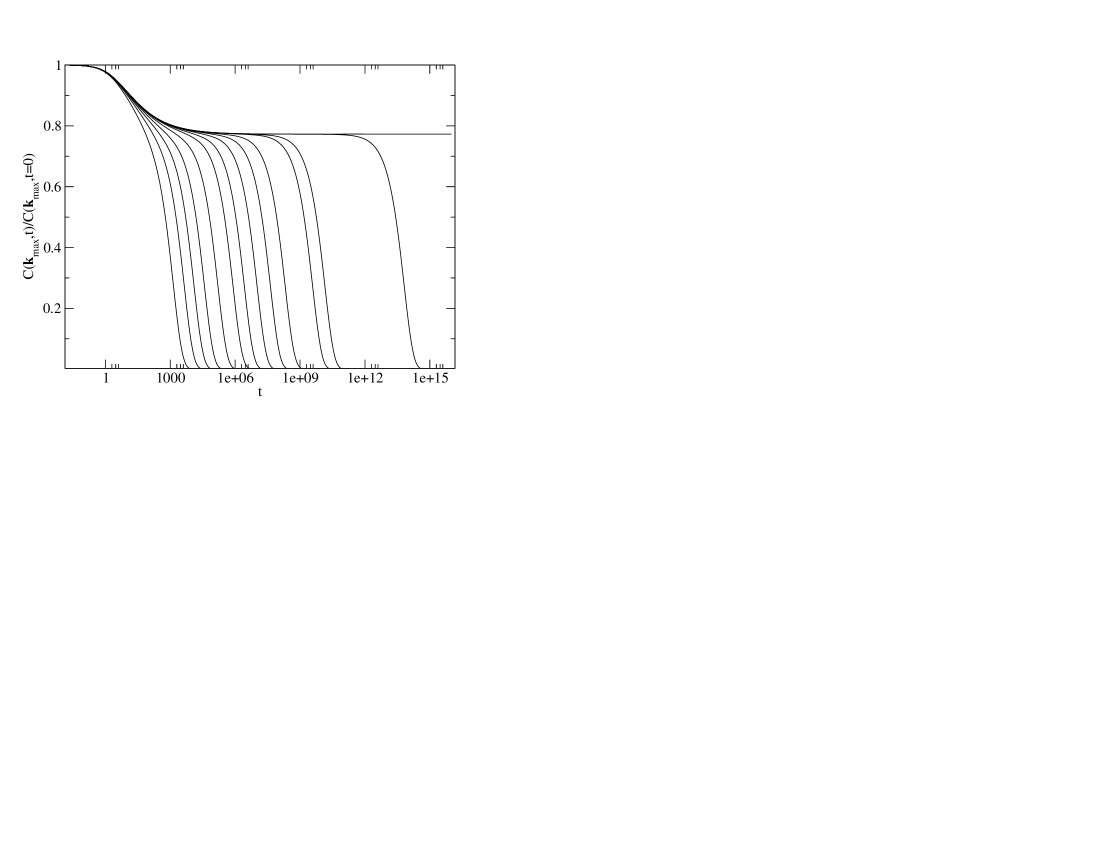
Figure 7: Time dependence of the correlation function $C({{\bf{k}}_{\max}},t)$ for $Q=0.1$ as predicted by the mode-coupling approximation (supplemented by the static Hartree approximation). Curves from left to right correspond to decreasing temperatures : $r_{0}=-1.05$, $-1.06$, $-1.065$, $-1.068$, $-1.070$, $-1.071$, $-1.07135$,$-1.07155$,$-1.07165$, $-1.0717$, $-1.07173$, $-1.071734$, $-1.0717379$, and $-1.071738$ .The dynamical transition is at $r_{0}\simeq-1.0717379\ldots$

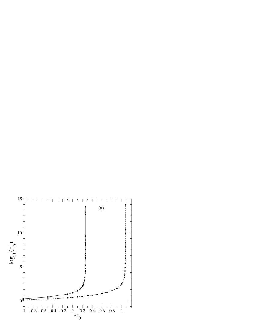
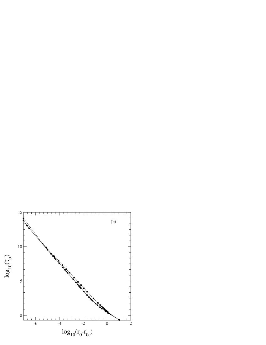
Figure 8: Temperature dependence of the $\alpha$-relaxation time $\tau_{\alpha}$ obtained from the dynamical mode-coupling prediction (with the static Hartree approximation) for the time dependent correlation function $C({\bf{k}_{\max}},t)$. $\tau_{\alpha}$ is defined as the time at which $C({\bf{k}_{\max}},t)=0.1$. Two frustrations, $Q=0.1$ and $Q=0.001$, are shown. (a) $\log_{10}(\tau_{\alpha})$ versus $-r_{0}$; the left and right curves correspond to $Q=0.1$ and $Q=0.001$ respectively. (b) $\log_{10}(\tau_{\alpha})$ versus $\log_{10}(r_{0}-r_{0c}(Q))$, where $r_{0c}(Q)$ is the ergodicity-breaking transition point.

VI Sensitivity of the results to the approximation scheme

We have already mentioned (see Ref. endnote3 ) that enough of the non-linearities of the original dynamical equation or of the equations in replica space must be kept in any approximate treatment in order to find non-trivial phenomena such as ergodicity breaking and appearance of an exponentially large number of metastable states. For this reason, the dynamical as well as the replica-space Hartree approximations are unable to generate such phenomena. One must therefore consider improved resummation schemes such as the mode-coupling approximation and the SCSAendnote4 .

The additional point we would like to make here is that even in the mode-coupling approximation, the results are somewhat dependent upon the supplementary approximation which is made to describe the static properties of the system entering as an input in the dynamical equation. It is well known, and was recalled above, that the location, or even the existence of an ergodicity-breaking transition is sensitive to the amplitude of the peak in the equilibrium (static) correlation function $C({{\bf{k}},t=0})$. We have seen that the Hartree and SCSA give slightly different, but compatible results. If one uses instead a somewhat less renormalized version of the SCSA with $\mu({\bf{k}})$ in Eq. (37) now defined with the Hartree and not the full correlation function, i.e.,

$$\mu({\bf{k}})=r_{0}+k^{2}+\frac{{{Q}}}{k^{2}}+u\int\frac{d^{3}{\bf q}}{(2\pi)^{3}}\frac{1}{\mu({\bf{q}})},$$ (40)

a different behavior is obtained. As shown in Fig. 9, the maximum of the static correlation function appears to saturate, as one lowers the temperature, to a value that is too small to trigger a breaking of ergodicity.

Finally, considering the static analog of the mode-coupling approximation to compute $C({{\bf{k}},t=0})$ (see Eq. (III) and below), i.e.,

$$C^{-1}({\bf{k}},t=0)= r_{0}+k^{2}+\frac{Q}{k^{2}}+3u\int\frac{d^{3}{\bf q}}{(2\pi)^{3}}C({\bf{q}},t=0)$$

$$- D({\bf{k}},t=0).$$ (41)

where $D({{\bf{k}},t=0})$ is given by Eq. (III) leads to a situation in which the limit of stability (spinodal) of the paramagnetic phase is reached at a finite temperature, before the occurrence of an ergodicity-breaking transition.

The validity of these various approximations should of course be checked by performing a computer simulation of the model. However, one can tentatively conclude from the above exercise that despite the formal similarity between the dynamics and the statics that comes from using the Martin-Siggia-Rose functional formalismMSR78 , different levels of approximation may be required to describe the dynamical and the static properties of the Coulomb frustrated model.

VII Conclusion

We have studied the Langevin dynamics of the soft-spin, continuum version of the Coulomb frustrated Ising ferromagnet. By using the dynamical mode-coupling approximation, coupled with reasonable approximations for describing the equilibrium static correlation function, and the dynamical self-consistent screening approximation, we have found that the system’s dynamics display a transition from ergodic to non-ergodic behavior, similar to that obtained in the idealized mode-coupling theory of glassforming liquidsgotze91 and in the mean-field generalized spin-glasses with one-step replica symmetry breakingKT87 ; BCKM96 . This transition occurs in the paramagnetic phase, either in the stable or the metastable region. It is related to the emergence of an exponentially large number of metastable states found by a purely static replica approach: the system looses ergodicity because it gets trapped in free-energy minima separated from each other by infinite barriers. This whole description, as can be inferred from the very nature of the approximations that amount to partial resummations of perturbative expansions, has a mean-field character: thermally activated processes are completely ignored. The predicted singularity is “avoided” in the true dynamics of the system and it remains to be seen, e.g., in computer simulations of Coulomb frustrated models, what signatures may still be observed in the time evolution of the correlation function. As for describing the activated processes, other, non-perturbative approaches, such as the phenomenological frustration-limited domainKKZNT95 and entropic-droplet picturesKTW89 , must be used.

Figure 9: Maximum of the correlation function $C({\bf{k}_{\max}},t)$ versus temperature ($r_{0}$) for $t=0$ (full lines) and $t\to\infty$ (dashed line) in the dynamical mode-coupling approximation. The value of the frustration is $Q=0.1$. The two upper curves correspond to the static Hartree approximation that predicts an ergodicity breaking transition. The lower curve that saturates at low temperatures corresponds to the less renormalized version of the SCSA (Eq. (40)): no dynamical transition is observed in this case.

Appendix A Fluctuation-induced first order transition

In this appendix, we calculate the temperature of the equilibrium transition between the paramagnetic phase and phases with spatially modulated order within the self-consistent Hartree approximation. The derivation given below closely follows Brazovskii’s original treatmentB75 .

The starting point is the Hamiltonian in Eq. (2) augmented by the introduction of spatially varying external fields $h_{{\bf{k}}}$ that are linearly coupled to the scalar field $\phi_{{\bf{k}}}$. As a result, $\phi_{{\bf{k}}}$ is now the sum of an average component, $m_{{\bf{k}}}=<\phi_{{\bf{k}}}>$, and a fluctuation $\psi_{{\bf{k}}}=\phi_{{\bf{k}}}-m_{{\bf{k}}}$. The self-consistent Hartree approximation is then equivalent to a gaussian variational approximation for the fluctuations. The resulting equation of state reads

$$h_{{\bf{k}}}= \left(r_{0}+k^{2}+\frac{Q}{k^{2}}\right)m_{{\bf{k}}}+u\int\frac{d^{3}{\bf k}_{1}}{(2\pi)^{3}}\int\frac{d^{3}{\bf k}_{2}}{(2\pi)^{3}}\left(m_{{\bf{k}_{1}}}m_{{\bf{k}_{2}}}+3C({\bf{k}_{1}},{\bf{k}_{2}})\right)m_{{\bf{k-k}_{1}-\bf{k}_{2}}},$$ (42)

where the connected correlation function $C({\bf{k}},{\bf{k}^{\prime}})=<\psi_{{\bf{k}}}\psi_{{\bf{k}}^{\prime}}>$, is obtained self-consistently by solving

$$C^{-1}({\bf{k}},{\bf{k}^{\prime}})=\left(r_{0}+k^{2}+\frac{Q}{k^{2}}\right)\delta({\bf{k}}+{\bf{k}^{\prime}})+3u\int\frac{d^{3}{\bf q}}{(2\pi)^{3}}\left(m_{{\bf{q}}}m_{{\bf{k+k^{\prime}-q}}}+C({\bf{q}},{\bf{k}}+{\bf{k}^{\prime}}-{\bf{q}})\right),$$ (43)

together with the inversion formula

$$\int\frac{d^{3}{\bf q}}{(2\pi)^{3}}C^{-1}({\bf{k}},{\bf{q}})C({\bf{q}},{\bf{k}^{\prime}})=\delta({\bf{k}^{\prime}}-{\bf{k}}).$$ (44)

In the paramagnetic phase when all $h_{{\bf{k}}}$’s, and therefore $m_{{\bf{k}}}$’s, are equal to zero, Eqs. (43) and (44) reduce to Eq. (5) with $C({\bf{k}},{\bf{k}^{\prime}})=C({\bf{k}})\delta({\bf{k}}+{\bf{k}^{\prime}})$.

In the vicinity of the transition between paramagnetic and modulated phases and for small enough frustration $Q$ ($Q<<1$), the modulated order is one-dimensional and characterized by a wave-vector ${\bf{k}}_{m}$ with $|{\bf{k}}_{m}|=k_{m}=Q^{1/4}$. It is then sufficient to consider

$$h_{{\bf{k}}}=\tilde{h}\left(\delta({\bf{k-k}_{m}})+\delta({\bf{k+k}_{m}})\right)$$ (45)

and

$$m_{{\bf{k}}}=\tilde{m}\left(\delta({\bf{k-k}_{m}})+\delta({\bf{k+k}_{m}})\right).$$ (46)

In this region, the fluctuations of wave-vector ${\bf{k}}$ with $|{\bf{k}}|=k_{m}$ are dominant, and BrazovskiiB75 has shown that the effect of the off-diagonal terms with ${\bf{k}}\neq{\bf{k}}^{\prime}$ could be neglected in the correlation function. As a result,

$$C({\bf{k}},{\bf{k}^{\prime}})\simeq\frac{\delta({\bf{k+k}^{\prime}})}{r+k^{2}+\frac{Q}{k^{2}}},$$ (47)

where the renormalized mass in a phase characterized by Eqs. (45,46), is given by:

$$r= r_{0}+3u\int\frac{d^{3}{\bf k}}{(2\pi)^{3}}\left(\frac{1}{r+k^{2}+\frac{Q}{k^{2}}}+|m_{{\bf{k}}}|^{2}\right)$$

$$= r_{0}+3u\int\frac{d^{3}{\bf k}}{(2\pi)^{3}}\frac{1}{r+k^{2}+\frac{Q}{k^{2}}}+6u|\tilde{m}|^{2}.$$ (48)

By introducing Eqs. (45)- (A) in Eq. (42) and recalling that $k_{m}=Q^{1/4}$, one obtains the following equation of state:

$$\tilde{h}= \left(r_{0}+2Q^{1/2}\right.$$

$$+ \left.3u\int\frac{d^{3}{\bf k}}{(2\pi)^{3}}\frac{1}{r+k^{2}+\frac{Q}{k^{2}}}+3u|\tilde{m}|^{2}\right)\tilde{m}$$

$$= \left(r+2Q^{1/2}-3u|\tilde{m}|^{2}\right)\tilde{m}.$$ (49)

In the Hartree approximation, and below some temperature, there is a coexistence of the paramagnetic phase and the modulated phase. In zero field ($\tilde{h}=0$), the former is characterized by $\tilde{m}=0$ and the latter by $\tilde{m}\neq 0$, where $\tilde{m}$ is solution of $\left(r+2Q^{1/2}-3u|\tilde{m}|^{2}\right)=0$. The transition point, which is then associated with a first-order transition, is obtained as the temperature at which the free-energies of the two phases are equal. Following BrazovskiiB75 , it is convenient to calculate directly the free-energy difference $\Delta F(r_{0})$ between the modulated ($\tilde{m}\neq 0$) and the paramagnetic ($\tilde{m}=0$) phases at a given temperature $r_{0}$ from the following expression:

$$\Delta F= \int_{0}^{\tilde{m}}d\tilde{m}^{\prime}\frac{\partial F}{\partial\tilde{m}^{\prime}}=2\int_{0}^{\tilde{m}}d\tilde{m}^{\prime}\tilde{h}(\tilde{m}^{\prime})$$ (50)

where $\tilde{h}_{\tilde{m}^{\prime}}$ is given by Eq. (A). One can change the integration variable from $\tilde{m}^{\prime}$ to $r^{\prime}$ with $r^{\prime}(\tilde{m}^{\prime})$ solution of Eq. (A). After some algebra, Eq. (50) can be recast as

$$u\Delta F= \int_{r(\tilde{m}=0)}^{r(\tilde{m})}d\tilde{r}^{\prime}\left(\frac{r^{\prime}+r_{0}}{2}+2Q^{1/2}+\frac{3u}{4\pi^{2}}\int dk\frac{k^{2}}{r+k^{2}+\frac{Q}{k^{2}}}\right)\left(\frac{1}{6}+\frac{u}{4\pi^{2}}\int dk\frac{k^{2}}{\left(r^{\prime}+k^{2}+\frac{Q}{k^{2}}\right)^{2}}\right),$$ (51)

where $r(\tilde{m}=0)$ is solution of Eq. (A) with $\tilde{m}=0$, i.e., of Eq. (6), and $r(\tilde{m})$ and $\tilde{m}$ are solutions of the two coupled equations, Eq. (A) and $\left(r+2Q^{1/2}-3u|\tilde{m}|^{2}\right)=0$. By solving Eq. (51) numerically for several values of $Q<<1$ (and for $u=1$), we have found that the sign of $\Delta F$ changes at a finite value of $r_{0}$ that marks the first-order transition between paramagnetic and modulated phases. The result is shown in Fig. 1. The transition being second-order in the mean-field approximation, it is then driven first-order by the fluctuations.

Appendix B Ergodicity breaking in the Dynamical SCSA

One can see from Eqs. (30)- (32) that ergodicity breaking requires that both $C({\bf{k}},t)$ and $C_{\sigma}({\bf{k}},t)$, and as a consequence $D({\bf{k}},t)$ and $D_{\sigma}({\bf{k}},t)$, go to non-zero values in the limit $t\to\infty$. From Eq. (34)), one obtains

$$C({\bf{k}},t\to\infty)=\frac{D({\bf{k}},t\to\infty)C({\bf{k}},0)^{2}}{1+D({\bf{k}},t\to\infty)C({\bf{k}},0)}.$$ (52)

A similar expression can be derived for $C_{\sigma}({\bf{k}},t\to\infty)$ by first Laplace transforming Eq. (III),

$$\hat{C}_{\sigma}({\bf{k}},z)=\frac{-C_{\sigma}({\bf{k}},0)}{z-\displaystyle\frac{1}{C_{\sigma}({\bf{k}},0)(i+\hat{D}_{\sigma}({\bf{k}},z))}}\,,$$ (53)

and by looking for the dominant behavior in the small-$z$ limit, $\hat{C}_{\sigma}({\bf{k}},z)\sim-C_{\sigma}({\bf{k}},t\to\infty)/z$, $\hat{D}_{\sigma}({\bf{k}},z)\sim-D_{\sigma}({\bf{k}},t\to\infty)/z$; one finally gets

$$C_{\sigma}({\bf{k}},t\to\infty)=\frac{-D_{\sigma}({\bf{k}},t\to\infty)C_{\sigma}({\bf{k}},0)^{2}}{1-D_{\sigma}({\bf{k}},t\to\infty)C_{\sigma}({\bf{k}},0)}.$$ (54)

By introducing the time-dependent polarization

$$\Pi({\bf{k}},t)=\int\frac{d^{3}{\bf{q}}}{(2\pi)^{3}}C({\bf{q}},t)C({\bf{k-q}},t),$$ (55)

one can express the memory kernel $D_{\sigma}({\bf{k}},t)$ given in Eq. (32) as

$$D_{\sigma}({\bf{k}},t)=-u\Pi({\bf{k}},t),$$ (56)

so that the $t=0$ and $t\to\infty$ values of $C_{\sigma}({\bf{k}},t)$ (given below Eq. (32) and in Eq. (54), respectively) can be written as

$$C_{\sigma}({\bf{k}},0)= \frac{-1}{1+u\Pi({\bf{k}},0)}$$ (57)

$$C_{\sigma}({\bf{k}},t\to\infty)= \frac{-u\Pi({\bf{k}},t\to\infty)C_{\sigma}({\bf{k}},0)^{2}}{1+u\Pi({\bf{k}},t\to\infty)C_{\sigma}({\bf{k}},0)}.$$ (58)

Recalling that $C({\bf{k}},0)=(\mu({\bf{k}})-D({\bf{k}},0))^{-1}$ with $\mu({\bf{k}})=r_{0}+k^{2}+Q/k^{2}+u\int\frac{d^{3}{\bf{q}}}{(2\pi)^{3}}C({\bf{q}},0)$ and that $D({\bf{k}},t)$ is given by Eq. (III), one obtains with Eqs. (52), (56) and (57) a closed set of equations that determines the non-ergodicity parameter $C({\bf{k}},t\to\infty)$. If one changes the notations from $C({\bf{k}},0)$ and $C({\bf{k}},t\to\infty)$ to $\cal{G}({\bf{k}})$ and $\cal{F}({\bf{k}})$, from $-D({\bf{k}},0)$ and $-D({\bf{k}},t\to\infty)$ to $\Sigma({\bf{k}})$ and $\Sigma_{\sigma}({\bf{k}})$, from $-uC({\bf{k}},0)$ and $-uC_{\sigma}({\bf{k}},t\to\infty)$ to ${\cal D}_{\cal G}({\bf{k}})$ and ${\cal D}_{\cal F}({\bf{k}})$, one can easily check that the above equations are identical to those obtained in RefsScWo00 ; SW201 with the replica formalism and the static SCSA.

References

- (1) D. Kivelson, S. A. Kivelson, X. L. Zhao, Z. Nussinov, and G. Tarjus, Physica A 219, 27 (1995); D. Kivelson, G. Tarjus, and S. A. Kivelson, Progress in Theo. Physics 126, 289 (1997).
- (2) P. Viot, G. Tarjus, and D. Kivelson, J. Chem. Phys. 112, 10368 (2000); G. Tarjus, D. Kivelson, and P. Viot, J. Phys: Cond. Mat. 12, 6497 (2000).
- (3) M. Grousson, G. Tarjus, and P. Viot, Phys. Rev. Lett. 86, 3455 (2001); M. Grousson, G. Tarjus, and P. Viot, cond-mat 0111305, (2001); M. Grousson, G. Tarjus, and P. Viot, J. Phys.: Cond. Mat. 14, 1617 (2002).
- (4) T. Ohta and K. Kawazaki, Macromolecules 19, 2621 (1986).
- (5) L. Leibler, Macromolecules 13, 1602 (1980).
- (6) G. H. Fredrickson and E. Helfand, J. Chem. Phys. 87, 697 (1987).
- (7) F. H. Stillinger, J. Chem. Phys. 78, 4654 (1983).
- (8) D. Wu, D. Chandler, and B. Smit, J. Phys. Chem. 96, 4077 (1992);H. J. Woo, C. Carraro, and D. Chandler, Phys. Rev. E 52, 6497 (1995).
- (9) V. J. Emery and S. A. Kivelson, Physica C 209, 597 (1993);U. Low, V. J. Emery, K. Fabricius, and S. A. Kivelson, Phys. Rev. Lett. 72, 1918 (1994).
- (10) J. Schmalian and P.G. Wolynes, Phys. Rev. Lett. 85, 836 (2000).
- (11) R. Monasson, Phys. Rev. Lett. 75, 2847 (1995).
- (12) M. Mézard and G. Parisi, Phys. Rev. Lett. 82, 747 (1999).
- (13) A. J. Bray, Phys. Rev. Lett. 32, 1413 (1974).
- (14) J. Schmalian and P.G. Wolynes, Phys. Rev. Lett. 86, 3456 (2001); H. Westfahl, J. Schmalian, and P.G. Wolynes, Phys. Rev. B 64, 174203 (2001).
- (15) One should note that is very close of , the relative difference being less than in the small frustration range, .
- (16) W. Götze, in Liquids, Freezing and the Glass transition, edited by J. P. H. D. Levesque and J. Zinn-Justin (North Holland, Amsterdam, 1991), p. 287.
- (17) H. Z. Cummins, J. Phys.: Cond. Mat. 11, 95 (1999).
- (18) T. R. Kirkpatrick and D. Thirumalai, Phys. Rev. Lett. 58, 2091 (1987).
- (19) J. P. Bouchaud, L. Cugliandolo, J. Kurchan, and M. Mézard, Physica A 226, 243 (1996).
- (20) A. Crisanti, H. Horner, and H. J. Sommers, Zeit. Phys. B 92, 257 (1993).
- (21) M. Grousson, G. Tarjus, and P. Viot, Phys. Rev. E 64, 036109 (2001).
- (22) S. A. Brazovskii, Sov. Phys. JETP 41, 85 (1975).
- (23) For a field theory with -component fields with symmetry, the Hartree approximation takes into account all diagrams that survive in the limit whereas the SCSA includes in a self-consistent manner the leading corrections. In the present case, one is of course interested by .
- (24) Contrary to those two approximations that retain some of the non-linearities of the dynamics, the dynamical counterpart of the Hartree approximation leads to an essentially linear equation, and it is not further considered in this work.
- (25) M. Campellone and J.-P. Bouchaud, J. Phys. A 30, 333 (1997).
- (26) M. Fuchs, W. Götze, I. Hofacker, and A. Latz, J. Phys.: Condens. Matter. 3, 5047 (1991).
- (27) V. Krakoviack, Ph.D. thesis, Univ. Paris Sud, Orsay, France, 2000.
- (28) P. Hohenberg and B. Halperin, Rev. Mod. Phys. 49, 435 (1977).
- (29) Note that the same considerations apply to the replica approach of the glassy state of simple liquids, where non-trivial behavior can be found with the hypernetted chain approximation, but not with the “too linear” Percus-Yevick and mean-spherical approximationsMP99 .
- (30) P.C. Martin, E.D. Siggia, and H.A. Rose, Phys. Rev. A 8, 423 (1973).
- (31) T. R. Kirkpatrick, D. Thirumalai, and P. G. Wolynes, Phys. Rev. A 40, 1045 (1989).