Thermodynamics and collapse of self-gravitating
Brownian particles in $D$ dimensions

Abstract

We address the thermodynamics (equilibrium density profiles, phase diagram, instability analysis…) and the collapse of a self-gravitating gas of Brownian particles in $D$ dimensions, in both canonical and microcanonical ensembles. In the canonical ensemble, we derive the analytic form of the density scaling profile which decays as $f(x)\sim x^{-\alpha}$, with $\alpha=2$. In the microcanonical ensemble, we show that $f$ decays as $f(x)\sim x^{-\alpha_{\rm max}}$, where $\alpha_{max}$ is a non-trivial exponent. We derive exact expansions for $\alpha_{\rm max}$ and $f$ in the limit of large $D$. Finally, we solve the problem in $D=2$, which displays rather rich and peculiar features.

1 Introduction

In an earlier paper [1], we studied a model of self-gravitating Brownian particles confined within a three-dimensional spherical box. We considered a high friction limit in which the equations of the problem reduce to a Smoluchowski-Poisson system with appropriate constraints ensuring the conservation of energy (in the microcanonical ensemble) or temperature (in the canonical ensemble) [2]. The equilibrium states (maximum entropy states) correspond to isothermal configurations which are known to exist only above a critical energy or a critical temperature (see, e.g., [3]). When no hydrostatic equilibrium exists, we found that the system generates a finite time singularity (i.e., the central density becomes infinite in a finite time) and we derived self-similar solutions describing the collapse. This study was performed both in the microcanonical and canonical ensembles, with emphasize on the inequivalence of ensembles for such a nonextensive system. In the canonical ensemble, we showed that the scaling exponent for the density is $\alpha=2$ and we determined the invariant profile $f(x)$, satisfying $f(x)\sim x^{-\alpha}$ for $x\rightarrow+\infty$, analytically. In the microcanonical ensemble, the scaling exponent $\alpha\simeq 2.21...$ and the corresponding invariant profile $f(x)$ were determined numerically.

In this paper, we propose to extend our analysis to a space of arbitrary dimension $D$. The interest of this extension is twofold. First, we shall consider an infinite dimension limit $D\rightarrow+\infty$ in which the problem can be solved analytically. In particular, it is possible to determine the scaling exponent $\alpha(D)$ and the profile $f(x,D)$ in the microcanonical ensemble by a systematic expansion procedure in powers of $D^{-1}$ (Sec. 3.4), while the canonical value is always $\alpha=2$ and the profile can be calculated exactly for any dimension (Sec. 3.3). We show that, already up to order $O(D^{-2})$, the results of the large $D$ expansion agree remarkably well with those found numerically for $D=3$. Moreover, we show that the nature of the problem changes at two particular dimensions $D=2$ and $D=10$. In Sec. 2, we compute the equilibrium phase diagram as a function of the dimension. For $2<D<10$, the $T-E$ curve has a spiral shape like in $3D$. For $D>10$ and $D<2$, the $T-E$ curve is monotonous. The dimension $D=2$ is critical and requires a particular attention that is given in Sec. 4. We show that for $D=2$ the system generates a Dirac peak (containing a finite fraction of mass) while for $D>2$, the central singularity contains no mass (at the collapse time). The case $D=2$ has interest in theoretical physics regarding 2D gravity [4] and string theory [5] (in connection with the Liouville field theory). It has also applications in the physics of random surfaces [6] and random potentials [7], 2D turbulence [8] and chemotaxis [9] (for bacterial populations). Finally, the dynamical equations considered in this paper and in Ref. [2] are receiving a growing interest from mathematicians who established rigorous results concerning the existence and unicity of solutions for arbitrary domain shape without specific symmetry. We refer to the papers of Rosier [10] and Biler et al. [11], and references therein, for the connection of our study with mathematical results.

2 Equilibrium structure of isothermal spheres in dimension $D$

2.1 The maximum entropy principle

Consider a system of particles with mass $m$ interacting via Newtonian gravity in a space of dimension $D$. The particles are enclosed within a box of radius $R$ so as to prevent evaporation and make a statistical approach rigorous. Let $f({\bf r},{\bf v},t)$ denote the distribution function of the system, i.e. $f({\bf r},{\bf v},t)d^{D}{\bf r}d^{D}{\bf v}$ gives the mass of particles whose position and velocity are in the cell $({\bf r},{\bf v};{\bf r}+d^{D}{\bf r},{\bf v}+d^{D}{\bf v})$ at time $t$. The integral of $f$ over the velocity determines the spatial density

(1) $$\rho=\int f\,d^{D}{\bf v}.$$

The total mass of the configuration is

(2) $$M=\int\rho\,d^{D}{\bf r}.$$

In the meanfield approximation, the total energy of the system can be expressed as

(3) $$E={1\over 2}\int fv^{2}\,d^{D}{\bf r}d^{D}{\bf v}+{1\over 2}\int\rho\Phi\,d^{D}{\bf r}=K+W,$$

where $K$ is the kinetic energy and $W$ the potential energy. The gravitational potential $\Phi$ is related to the density by the Newton-Poisson equation

(4) $$\Delta\Phi=S_{D}G\rho,$$

where $S_{D}$ is the surface of a unit sphere in a $D$-dimensional space and $G$ is the constant of gravity. Finally, we introduce the Boltzmann entropy

(5) $$S=-\int f\ln f\,d^{D}{\bf r}d^{D}{\bf v},$$

and the free energy (more precisely the Massieu function)

(6) $$J=S-\beta E,$$

where $\beta=1/T$ is the inverse temperature. If the system is isolated, the equilibrium state maximizes the entropy $S$ at fixed energy $E$ and mass $M$ (microcanonical description). Alternatively, if the system is in contact with a heat bath which maintains its temperature fixed, the equilibrium state maximizes the free energy $J$ at fixed mass $M$ and temperature $T$ (canonical description). It can be shown that for systems interacting via a long-range potential like gravity, this meanfield description is exact so that our “thermodynamical approach” is rigorous.

To solve this variational problem, we shall proceed in two steps. We first maximize $S$ (resp. $J$) at fixed $M$, $E$ (resp. $T$) and $\rho({\bf r})$. This yields the Maxwell distribution

(7) $$f={1\over(2\pi T)^{D/2}}\rho({\bf r})e^{-{v^{2}\over 2T}}.$$

It is now possible to express the energy and the entropy in terms of $\rho({\bf r})$ as

(8) $$E={D\over 2}MT+{1\over 2}\int\rho\Phi d^{D}{\bf r},$$

(9) $$S={D\over 2}M\ln T-\int\rho\ln\rho d^{D}{\bf r},$$

where we have omitted unimportant constant terms in the entropy (9). The entropy and the free energy are now functionals of $\rho({\bf r})$ and we consider their maximization at fixed energy or temperature. Introducing Lagrange multipliers to satisfy the constraints, the critical points of $S$ or $J$ are given by the Boltzmann distribution

(10) $$\rho=Ae^{-\beta\Phi}.$$

Then, the equilibrium state is obtained by solving the Boltzmann-Poisson equation

(11) $$\Delta\Phi=S_{D}GAe^{-\beta\Phi},$$

and relating the Lagrange multipliers to the appropriate constraints. Note that a similar variational problem occurs in the context of two-dimensional turbulence ($D=2$) to characterize large-scale vortices considered as maximum entropy structures [12, 2, 13].

It is easy to show that there is no global maximum of entropy at fixed mass and energy for $D>2$ (see, e.g., Ref. [1] for $D=3$). We can make the entropy diverge to $+\infty$ by approaching an arbitrarily small fraction of particles in the core ($M_{core}\ll M$) so that the potential energy goes to $-\infty$. Since the total energy is conserved, the temperature must rise to $+\infty$ and this leads to a divergence of the entropy to $+\infty$. Note that if we collapse all particles in the core, the entropy would diverge to $-\infty$. Therefore, the formation of a Dirac peak is not thermodynamically favorable in the microcanonical ensemble. For $D=2$, there exists a global entropy maximum for all energies. On the other hand, there is no global maximum of free energy at fixed mass and temperature for $D>2$ (see, e.g., Ref. [18] for $D=3$) and if $T<T_{c}=GM/4$ for $D=2$ (see Appendix A). We can make the free energy $J$ diverge to $+\infty$ by collapsing all particles at $r=0$. Therefore, a canonical system is expected to form a Dirac peak. For $D=2$ and $T>T_{c}$, there exists a global maximum of free energy. For $D<2$, there exists a global maximum of entropy and free energy for all accessible values of energy and temperature. We refer to Refs. [14, 15] for a rigorous proof of these results. When no global maxima of entropy or free energy exist, we can nevertheless look for local maxima since they correspond to metastable states which can be relevant for the considered time scales. Of course, the critical points of entropy at fixed $E$ and $M$ are the same as the critical point of free energy at fixed $T$ and $M$. Only the onset of instability (regarding the second order variations of $S$ or $J$ with appropriate constraints) will differ from one ensemble to the other. For $D=3$, this stability problem was considered by Antonov [16] and Padmanabhan [17] in the microcanonical ensemble and by Chavanis [18] in the canonical ensemble, by solving an eigenvalue equation. It was also studied by Lynden-Bell & Wood [19] and Katz [20] by using an extension of Poincaré theory of linear series of equilibria. We shall give the generalization of these results in Sec. 2.6 to the case of a system of arbitrary dimension $D$.

2.2 The $D$-dimensional Emden equation

To determine the structure of isothermal spheres, we introduce the function $\psi=\beta(\Phi-\Phi_{0})$, where $\Phi_{0}$ is the gravitational potential at $r=0$. Then, the density field can be written

(12) $$\rho=\rho_{0}e^{-\psi},$$

where $\rho_{0}$ is the central density. Introducing the notation $\xi=(S_{D}G\beta\rho_{0})^{1/2}r$ and restricting ourselves to spherically symmetrical configurations (which maximize the entropy for a non-rotating system), the Boltzmann-Poisson Eq. (11) reduces to the form

(13) $${1\over\xi^{D-1}}{d\over d\xi}\biggl{(}\xi^{D-1}{d\psi\over d\xi}\biggr{)}=e^{-\psi},$$

which is the $D$-dimensional generalization of the Emden equation [21]. For $D>2$, Eq. (13) has a simple explicit solution, the singular sphere

(14) $$e^{-\psi_{s}}={2(D-2)\over\xi^{2}}.$$

The regular solution of Eq. (13) satisfying the boundary conditions

(15) $$\psi=\psi^{\prime}=0\qquad{\rm at}\qquad\xi=0,$$

must be computed numerically. For $\xi\rightarrow 0$, we can expand the solution in Taylor series and we find that

(16) $$\psi={1\over 2D}\xi^{2}-{1\over 8D(D+2)}\xi^{4}+{1\over 24}{D+1\over D^{2}(D+2)(D+4)}\xi^{6}+...$$

To obtain the asymptotic behavior of the solutions for $\xi\rightarrow+\infty$, we note that the transformation $t=\ln\xi$, $\psi=2\ln\xi-z$ changes Eq. (13) in

(17) $${d^{2}z\over dt^{2}}+(D-2){dz\over dt}=-e^{z}+2(D-2).$$

For $D>2$, this corresponds to the damped oscillations of a fictitious particle in a potential $V(z)=e^{z}-2(D-2)z$, where $z$ plays the role of the position and $t$ the role of time. For $t\rightarrow+\infty$, the particle will come at rest at the bottom of the well at position $z_{0}=\ln(2(D-2))$. Returning to original variables, we find that

(18) $$e^{-\psi}\rightarrow{2(D-2)\over\xi^{2}}=e^{-\psi_{s}},\qquad{\rm for}\qquad\xi\rightarrow+\infty.$$

Therefore, the regular solution of the Emden equation (13) behaves like the singular solution for $\xi\rightarrow+\infty$. To determine the next order correction, we set $z=z_{0}+z^{\prime}$ with $z^{\prime}\ll 1$. Keeping only terms that are linear in $z^{\prime}$, Eq. (17) becomes

(19) $${d^{2}z^{\prime}\over dt^{2}}+(D-2){dz^{\prime}\over dt}+2(D-2)z^{\prime}=0.$$

The discriminant associated with this equation is $\Delta=(D-2)(D-10)$. It exhibits two critical dimensions $D=2$ and $D=10$. For $2<D<10$, we have

(20) $$e^{-\psi}={2(D-2)\over\xi^{2}}\biggl{\{}1+{A\over\xi^{{D-2\over 2}}}\cos\biggl{(}{\sqrt{(D-2)(10-D)}\over 2}\ln\xi+\delta\biggr{)}\biggr{\}},\qquad(\xi\rightarrow+\infty).$$

The density profile (20) intersects the singular solution (14) infinitely often at points that asymptotically increase geometrically in the ratio $1:e^{2\pi/\sqrt{(D-2)(10-D)}}$ (see, e.g., Fig. 1 of Ref. [18] for $D=3$). For $D\geq 10$, we have

(21) $$e^{-\psi}={2(D-2)\over\xi^{2}}\biggl{\{}1+{1\over\xi^{{D-2\over 2}}}\biggl{(}A\xi^{\sqrt{(D-2)(10-D)}\over 2}+B\xi^{-\sqrt{(D-2)(10-D)}\over 2}\biggr{)}\biggr{\}},\qquad(\xi\rightarrow+\infty).$$

For $D=2$, Eq. (17) can be solved explicitly and we get

(22) $$e^{-\psi}={1\over(1+{1\over 8}\xi^{2})^{2}}.$$

This result has been found by various authors in different fields (see, e.g., [4, 22]). Note that $e^{-\psi}\sim\xi^{-4}$ at large distances instead of the usual $\xi^{-2}$ behavior obtained for $D>2$. This implies that the mass of an unbounded isothermal sphere is finite in $D=2$, although it is infinite for $D>2$.

For $D<2$, we can neglect the r.h.s. in Eq. (18) and we get

(23) $$e^{-\psi}\sim e^{-A_{D}\xi^{2-D}},\qquad(\xi\rightarrow+\infty),$$

where $A_{D}$ is a constant depending on the dimension $D$. For $D=1$, Eq. (13) can be solved exactly, yielding the result

(24) $$e^{-\psi}={1\over\cosh^{2}(\xi/\sqrt{2})},$$

establishing $A_{1}=\sqrt{2}$.

2.3 The Milne variables

As is well-known [21], isothermal spheres satisfy a homology theorem: if $\psi(\xi)$ is a solution of the Emden equation, then $\psi(A\xi)-2\ln A$ is also a solution, with $A$ an arbitrary constant. This means that the profile of isothermal configurations is always the same (characterized intrinsically by the function $\psi$), provided that the central density and the typical radius are rescaled appropriately. Because of this homology theorem, the second order differential equation (13) can be reduced to a first order differential equation for the Milne variables

(25) $$u={\xi e^{-\psi}\over\psi^{\prime}}\qquad{\rm and}\qquad v=\xi\psi^{\prime}.$$

Taking the logarithmic derivative of $u$ and $v$ with respect to $\xi$ and using Eq. (13), we get

(26) $${1\over u}{du\over d\xi}={1\over\xi}(D-v-u),$$

(27) $${1\over v}{dv\over d\xi}={1\over\xi}(2-D+u).$$

Taking the ratio of the foregoing equations, we obtain

(28) $${u\over v}{dv\over du}={2-D+u\over D-u-v}.$$

The solution curve in the $(u,v)$ plane is plotted in Fig. 1 for different values of $D$. The curve is parameterized by $\xi$. It starts from the point $(u,v)=(D,0)$ with a slope $(dv/du)_{0}=-(D+2)/D$ corresponding to $\xi=0$. The points of horizontal tangent are determined by $u=D-2$ and the points of vertical tangent by $u+v=D$. These two lines intersect at $(u_{s},v_{s})=(D-2,2)$, which corresponds to the singular solution (14). For $2<D<10$, the solution curve spirals indefinitely around the point $(u_{s},v_{s})$. For $D\geq 10$, the curve reaches the point $(u_{s},v_{s})$ without spiraling. For $D=2$, we have the explicit solution $v=2(2-u)$ so that $(u,v)\rightarrow(0,4)$ for $\xi\rightarrow+\infty$. For $D<2$, $(u,v)\rightarrow(0,+\infty)$ for $\xi\rightarrow+\infty$ (see Fig. 2). More precisely,

(29) $${ue^{v\over 2-D}\over v^{D\over 2-D}}\sim\omega_{D},\qquad(\xi\rightarrow+\infty),$$

where we have defined $\omega_{D}=1/(A_{D}(2-D)^{2\over 2-D})$. For $D=1$, $\omega_{1}=1/\sqrt{2}$.

Figure 1: The solutions of the Emden equation in the $(u,v)$ plane for systems with dimension $2<D<10$.

Figure 2: The solutions of the Emden equation in the $(u,v)$ plane for systems with dimension $D=1$ and $D=2$.

2.4 The thermodynamical parameters

For bounded isothermal systems, the solution of Eq. (13) is terminated by the box at a normalized radius given by $\alpha=(S_{D}\beta\rho_{0})^{1/2}R$. We shall now relate the parameter $\alpha$ to the temperature and energy. According to the Poisson equation (4), we have

(30) $$GM=\int G\rho d^{D}{\bf r}=\int_{0}^{R}S_{D}G\rho r^{D-1}dr=\int_{0}^{R}{d\over dr}\biggl{(}r^{D-1}{d\Phi\over dr}\biggr{)}dr=\biggl{(}r^{D-1}{d\Phi\over dr}\biggr{)}_{r=R}.$$

Introducing the dimensionless variables defined previously (using $r/R=\xi/\alpha$), we get

(31) $$\eta\equiv{\beta GM\over R^{D-2}}=\alpha\psi^{\prime}(\alpha).$$

We note that, for $D=2$, the parameter $\eta$ is independent on $R$. This is a consequence of the logarithmic form of the Newtonian potential in two dimensions.

The computation of the energy is a little more intricate. First, using an extension of the potential tensor theory developed by Chandrasekhar (see, e.g., Ref. [23]), we can show that the potential energy in $D$-dimensions can be written

(32) $$W=-{1\over D-2}\int\rho\ {\bf r}\cdot\nabla\Phi d^{D}{\bf r},$$

for $D\neq 2$. Now, the Boltzmann-Poisson equation (11) is equivalent to the condition of hydrostatic equilibrium

(33) $$\nabla p=-\rho\nabla\Phi,$$

with an equation of state $p=\rho T$. Substituting this relation in Eq. (32) and integrating by parts, we obtain

(34) $$2K+(D-2)W=DV_{D}R^{D}p(R),$$

where $V_{D}=S_{D}/D$ is the volume of a hypersphere with unit radius. Eq. (34) is the form of the Virial theorem in $D$-dimension. The total energy $E=K+W$ can be written

(35) $$E={D-4\over D-2}K+{D\over D-2}V_{D}R^{D}p(R).$$

Expressing the pressure in terms of the Emden function, using $p=\rho T$ and Eq. (12), and using Eq. (31) to eliminate the temperature, we finally obtain

(36) $$\Lambda\equiv-{ER^{D-2}\over GM^{2}}={D(4-D)\over 2(D-2)}{1\over\alpha\psi^{\prime}(\alpha)}-{1\over D-2}{e^{-\psi(\alpha)}\over\psi^{\prime}(\alpha)^{2}}.$$

It turns out that the normalized temperature and the normalized energy can be expressed very simply in terms of the values of the Milne variables at the normalized box radius. Indeed, writing $u_{0}=u(\alpha)$ and $v_{0}=v(\alpha)$ and using Eqs. (31)(36), we get

(37) $$\eta=v_{0},$$

(38) $$\Lambda={1\over v_{0}}\biggl{[}{D(4-D)\over 2(D-2)}-{u_{0}\over D-2}\biggr{]}.$$

Figure 3: Evolution of the inverse temperature $\eta$ along the series of equilibrium (parameterized by $\alpha$) for $2<D<10$. The curves correspond to $D=4,3,2.5,2.2$ from bottom to top.

Figure 4: Evolution of the energy $\Lambda$ along the series of equilibria (parameterized by $\alpha$) for $2<D<10$.

The curves $\eta(\alpha)$, $\Lambda(\alpha)$ are plotted in Figs. 3-4. For $2<D<10$, they exhibit damped oscillations toward the values $\eta_{s}=2$ and $\Lambda_{s}=1/(D-2)-D/4$, corresponding to the singular solution (14). For $D\geq 10$ the curves are monotonous. For $D=2$, we have explicitly

(39) $$\eta={\alpha^{2}\over 2(1+{1\over 8}\alpha^{2})},\qquad\Lambda={2\over\alpha^{2}}\biggl{(}1+{\alpha^{2}\over 8}\biggr{)}\biggl{\{}{8\over\alpha^{2}}\biggl{(}1+{\alpha^{2}\over 8}\biggr{)}\ln\biggl{(}1+{\alpha^{2}\over 8}\biggr{)}-2\biggr{\}}.$$

The expression of the energy has been obtained directly from Eq. (8) with the boundary condition $\Phi(R)=0$. The inverse temperature increases monotonically with $\alpha$ up to the value $\eta_{c}=4$. Using Eq. (22) and returning to the original variables, we can write the density profile in the form

(40) $$\rho={4M\over\pi R^{2}(4-\eta)(1+{\eta\over 4-\eta}{r^{2}\over R^{2}})^{2}}.$$

This density profile is represented in Fig. 5 for different temperatures. At the critical inverse temperature $\eta_{c}=4$, all the particles are concentrated at the center of the domain. The density profile approaches the Dirac distribution

(41) $$\rho({\bf r})\rightarrow M\delta({\bf r})\qquad{\rm for}\qquad\eta\rightarrow\eta_{c}=4,$$

which has an infinite (negative) energy.

For $D<2$, the curves $\eta(\alpha)$ and $\Lambda(\alpha)$ tend to $+\infty$ and $0$ as $\alpha\rightarrow+\infty$. For $D=1$, we have explicitly

(42) $$\eta=2\sqrt{2}\alpha\tanh(\alpha/\sqrt{2}),\qquad\Lambda=-{3\over 4\sqrt{2}}{1\over\alpha\tanh(\alpha/\sqrt{2})}+{1\over 8}{1\over\sinh^{2}(\alpha/\sqrt{2})}.$$

Note that according to Eq. (32), the energy is necessarily positive for $D<2$, so the region $\Lambda\geq 0$ is forbidden. Returning to original variables, the density profile is given by

(43) $$\rho={M\over 4\sqrt{2}R}\ {\alpha\over\tanh(\alpha/\sqrt{2})}\ {1\over\cosh^{2}\bigl{(}{\alpha r\over\sqrt{2}R}\bigr{)}},$$

where we recall that $S_{1}=2$. For $\alpha\rightarrow+\infty$, the profile tends to a Dirac peak $M\delta(r)$.

Figure 5: Equilibrium density profile of a two-dimensional self-gravitating system as a function of the inverse temperature $\eta$. For $\eta=0$, the density is uniform. For $\eta\rightarrow\eta_{c}=4$, the density tends to a Dirac peak. For $\eta>\eta_{c}$, there is no equilibrium state.

In Figs. 6-7, we have plotted the equilibrium phase diagram $\Lambda-\eta$, giving the temperature as a function of the energy, for different dimensions $D$. For $2<D<10$, the curve spirals around the limit point $(\Lambda_{s},\eta_{s})$ corresponding to the singular solution. For $D\geq 10$, the curve is monotonous until the limit point. For $D=2$, the curve is explicitly given by

(44) $$\Lambda={1\over\eta}\biggl{[}{4\over\eta}\ln\biggl{(}{4\over 4-\eta}\biggr{)}-2\biggr{]},$$

and is represented in Fig. 7, together with the case $D=1$.

We stress that the preceding results, obtained in the meanfield approximation, are exact in the thermodynamical limit $N\rightarrow+\infty$ such that $\eta$ and $\Lambda$ are kept fixed. If the box radius is given, this implies that $T\sim N$ and $E\sim N^{2}$. Alternatively, if the temperature and the energy per particle are given, the thermodynamical limit is such that $N\rightarrow+\infty$ with $N/R^{D-2}$ constant (for $D>2$).

Figure 6: Equilibrium phase diagram giving the inverse temperature $\eta$ as a function of minus the energy $\Lambda$ for systems with dimension $2<D<10$.

Figure 7: Equilibrium phase diagram for two-dimensional self-gravitating systems. For infinitely negative energies, the inverse temperature tends to the value $\eta_{c}=4$.

2.5 The minimum temperature and minimum energy

For $2<D<10$, the curve $\eta(\alpha)$ presents an extremum at points $\alpha_{n}$ such that $d\eta/d\alpha(\alpha_{n})=0$. Using Eqs. (37) and (27), we find that this condition is equivalent to

(45) $$u_{0}=D-2=u_{s}.$$

Since the curve $u=u_{s}$ passes through the center of the spiral in the $(u,v)$ plane, this determines an infinity of solutions (see Fig. 8), one at each extremum of $v$ (since $\eta=v_{0}$). Asymptotically, the $\alpha_{n}$ follow a geometric progression (see Ref. [18] for more details):

(46) $$\alpha_{n}\sim e^{2\pi n/\sqrt{(D-2)(10-D)}},\qquad(n\rightarrow+\infty,\ {\rm integer}).$$

In Fig. 3, we see that an equilibrium state exists only for

(47) $$\eta={\beta GM\over R^{D-2}}\leq\eta(\alpha_{1}),\qquad(2<D<10).$$

This determines a maximum mass (for given $T$ and $R$) or a minimum temperature (for given $M$ and $R$) beyond which no equilibrium state is possible. In that case, the system is expected to undergo an isothermal collapse (see Sect. 3.3). For $D=2$ and for $D\geq 10$, the $\eta(\alpha)$ curve is monotonous. An equilibrium state exists only provided that

(48) $$\eta={\beta GM}\leq\eta_{c}=4,\qquad(D=2),$$

(49) $$\eta={\beta GM\over R^{D-2}}\leq\eta_{s}=2,\qquad(D\geq 10).$$

Figure 8: Location of the turning points of energy and temperature in the $(u,v)$ plane for systems with dimension $2<D<10$. The construction is made explicitly for $D=3$, which corresponds to the case extensively studied in Refs. [17, 18]. The dashed line $v=2$ determines the location of the nodes of the density profiles that trigger the instabilities (see Sec. 2.6).

We get comparable results for the energy. For $2<D<10$, the curve $\Lambda(\alpha)$ presents an extremum at points $\alpha^{\prime}_{n}$ such that $d\Lambda/d\alpha(\alpha^{\prime}_{n})=0$. Using Eqs. (38) and (26)(27), we find that this condition is equivalent to

(50) $$4u_{0}^{2}+2u_{0}v_{0}+(D^{2}-8D+4)u_{0}+D(D-2)(4-D)=0.$$

We can check that the limit point $(u_{s},v_{s})$ is solution of this equation. Therefore, the intersection of the parabola $(P)$ defined by Eq. (50) with the spiral in the $(u,v)$ plane determines an infinity of points $\alpha^{\prime}_{n}$ at which the energy is extremum (see Fig. 8). On Fig. 4, we see that an equilibrium state exists only for

(51) $$\Lambda={-ER^{D-2}\over GM^{2}}\leq\Lambda(\alpha^{\prime}_{1}),\qquad(2<D<10).$$

This determines a minimum energy (for given $M$ and $R$) or a maximum radius (for given $M$ and $E$) beyond which no equilibrium state exists. In that case, the system is expected to collapse and overheat; this is called gravothermal catastrophe (see Sect. 3.4). For $D\geq 10$, the curve $\Lambda(\alpha)$ is monotonous. An equilibrium state exist only for

(52) $$\Lambda={-ER^{D-2}\over GM^{2}}\leq\Lambda_{s}={1\over D-2}-{D\over 4},\qquad(D\geq 10).$$

For $D=2$, there exists an equilibrium state for each value of energy (see Fig. 7): there is no gravothermal catastrophe in the microcanonical ensemble in two-dimensions [4]. For $D<2$, there exists an equilibrium state for all accessible values of energy and temperature.

2.6 The thermodynamical stability

We now study the thermodynamical stability of self-gravitating systems in various dimensions. We start by the canonical ensemble which is simpler in a first approach. A critical point of free energy at fixed mass and temperature is a local maximum if, and only if, the second order variations

(53) $$\delta^{2}J=-\int{(\delta\rho)^{2}\over 2\rho}d^{D}{\bf r}-{1\over 2T}\int\delta\rho\delta\Phi d^{D}{\bf r},$$

are negative for any variation $\delta\rho$ that conserves mass to first order, i.e.

(54) $$\int\delta\rho d^{D}{\bf r}=0.$$

This is the condition of thermodynamical stability in the canonical ensemble. Introducing the function $q(r)$ by the relation

(55) $$\delta\rho={1\over S_{D}r^{D-1}}{dq\over dr},$$

and following a procedure similar to the one adopted in Ref. [18], we can put the second order variations of free energy in the quadratic form

(56) $$\delta^{2}J={1\over 2}\int_{0}^{R}drq\biggl{[}{G\over Tr^{D-1}}+{d\over dr}\biggl{(}{1\over S_{D}\rho r^{D-1}}{d\over dr}\biggr{)}\biggr{]}q.$$

The second order variations of free energy can be positive (implying instability) only if the differential operator which occurs in the integral has positive eigenvalues. We need therefore to consider the eigenvalue problem

(57) $$\biggl{[}{d\over dr}\biggl{(}{1\over S_{D}\rho r^{D-1}}{d\over dr}\biggr{)}+{G\over Tr^{D-1}}\biggr{]}q_{\lambda}(r)=\lambda q_{\lambda}(r).$$

with $q_{\lambda}(0)=q_{\lambda}(R)=0$. If all the eigenvalues $\lambda$ are negative, then the critical point is a maximum of free energy. If at least one eigenvalue is positive, the critical point is an unstable saddle point. The point of marginal stability, i.e. the value of $\alpha$ in the series of equilibria $\eta(\alpha)$ at which the solutions pass from local maxima of free energy to unstable saddle points, is determined by the condition that the largest eigenvalue is equal to zero ($\lambda=0$). We thus have to solve the differential equation

(58) $${d\over dr}\biggl{(}{1\over S_{D}\rho r^{D-1}}{dF\over dr}\biggr{)}+{GF\over Tr^{D-1}}=0,$$

with $F(0)=F(R)=0$. Introducing the dimensionless variables defined previously, we can rewrite this equation in the form

(59) $${d\over d\xi}\biggl{(}{e^{\psi}\over\xi^{D-1}}{dF\over d\xi}\biggr{)}+{F(\xi)\over\xi^{D-1}}=0,$$

with $F(0)=F(\alpha)=0$. If

(60) $${\cal L}\equiv{d\over d\xi}\biggl{(}{e^{\psi}\over\xi^{D-1}}{d\over d\xi}\biggr{)}+{1\over\xi^{D-1}}$$

denotes the differential operator which occurs in Eq. (59), we can check by using the Emden Eq. (13) that

(61) $${\cal L}(\xi^{D-1}\psi^{\prime})=\psi^{\prime},\qquad{\cal L}(\xi^{D}e^{-\psi})=(D-2)\psi^{\prime}.$$

Therefore, the general solution of Eq. (59) satisfying the boundary conditions at $\xi=0$ is

(62) $$F(\xi)=c_{1}(\xi^{D}e^{-\psi}-(D-2)\xi^{D-1}\psi^{\prime}).$$

Using Eq. (62) and introducing the Milne variables (25), the condition $F(\alpha)=0$ can be written

(63) $$u_{0}=D-2.$$

This relation determines the points at which a new eigenvalue becomes positive (crossing the line $\lambda=0$). Comparing with Eq. (45), we see that a mode of stability is lost each time that $\eta$ is extremum in the series of equilibria, in agreement with the turning point criterion of Katz [20] in the canonical ensemble. In particular, the series becomes unstable at the point of minimum temperature (or maximum mass) $\alpha_{1}$. Secondary modes of instability appear at values $\alpha_{2}$, $\alpha_{3}$,… We obtain the same results by considering the dynamical stability of isothermal gaseous spheres with respect to the Navier-Stokes equations (see Ref. [18] for $D=3$). Therefore, dynamical and thermodynamical stability criteria coincide for isothermal gaseous spheres.

According to Eq. (55), the perturbation profile that triggers a mode of instability at the critical point $\lambda=0$ is given by

(64) $${\delta\rho\over\rho_{0}}={1\over S_{D}\xi^{D-1}}{dF\over d\xi},$$

where $F(\xi)$ is given by Eq. (62). Introducing the Milne variables (25), we get

(65) $${\delta\rho\over\rho}={c_{1}\over S_{D}}(2-v).$$

The density perturbation $\delta\rho$ becomes zero at point(s) $\xi_{i}$ such that $v(\xi_{i})=2$. The number of zeros is therefore given by the number of intersections between the spiral in the $(u,v)$ plane and the line $v=2$ (see Fig. 8). For the $n$-th mode of instability we need to follow the spiral to the $n$-th extremum of $v$ (since $\alpha_{n}$ corresponds to an extremum of $\eta$, hence $v$). Therefore, the density perturbation $\delta\rho$ corresponding to the $n$-th mode of instability has $n$ zeros $\xi_{1},\xi_{2},...,\xi_{n}<\alpha_{n}$. Asymptotically, the zeros follow a geometric progression with ratio $e^{2\pi/\sqrt{(D-2)(10-D)}}$ [18].

In the microcanonical ensemble, the condition of thermodynamical stability requires that the equilibrium state is an entropy maximum at fixed mass and energy. This condition can be written

(66) $$\delta^{2}S=-\int{(\delta\rho)^{2}\over 2\rho}d^{D}{\bf r}-{1\over 2T}\int\delta\rho\delta\Phi d^{D}{\bf r}-{1\over DMT^{2}}\biggl{(}\int\Phi\delta\rho d^{D}{\bf r}\biggr{)}^{2}<0,$$

for any variation $\delta\rho$ that conserves mass to first order (the conservation of energy has already been taken into account in obtaining Eq. (66)). Now, following a procedure similar to that of Ref. [3] in $D=3$, the second variations of entropy can be put in a quadratic form

(67) $$\delta^{2}S=\int_{0}^{R}\int_{0}^{R}drdr^{\prime}q(r)K(r,r^{\prime})q(r^{\prime}),$$

with

(68) $$K(r,r^{\prime})=-{1\over DMT^{2}}{d\Phi\over dr}(r){d\Phi\over dr}(r^{\prime})+{1\over 2}\delta(r-r^{\prime})\biggl{[}{G\over Tr^{D-1}}+{d\over dr}\biggl{(}{1\over S_{D}\rho r^{D-1}}{d\over dr}\biggr{)}\biggr{]}.$$

The problem of stability can therefore be reduced to the study of the eigenvalue equation

(69) $$\int_{0}^{R}dr^{\prime}K(r,r^{\prime})F_{\lambda}(r^{\prime})=\lambda F_{\lambda}(r),$$

with $F_{\lambda}(0)=F_{\lambda}(R)=0$. The point of marginal stability ($\lambda=0$) will be determined by solving the differential equation

(70) $${d\over dr}\biggl{(}{1\over S_{D}\rho r^{D-1}}{dF\over dr}\biggr{)}+{GF\over Tr^{D-1}}={2V\over DMT^{2}}{d\Phi\over dr}(r),$$

with

(71) $$V=\int_{0}^{R}{d\Phi\over dr}(r^{\prime})F(r^{\prime})dr^{\prime}.$$

Introducing the dimensionless variables defined previously, this is equivalent to

(72) $${d\over d\xi}\biggl{(}{e^{\psi}\over\xi^{D-1}}{dF\over d\xi}\biggr{)}+{F\over\xi^{D-1}}=\chi{d\psi\over d\xi},$$

with

(73) $$\chi={2\over D\alpha^{D-1}\psi^{\prime}(\alpha)}\int_{0}^{\alpha}{d\psi\over d\xi}(\xi^{\prime})F(\xi^{\prime})d\xi^{\prime},$$

and $F(0)=F(\alpha)=0$. Using the identities (61), we can check that the general solution of Eq. (72) satisfying the boundary conditions for $\xi=0$ and $\xi=\alpha$ is

(74) $$F(\xi)={\chi\over D-2-u_{0}}\biggl{(}\xi^{D}e^{-\psi}-(D-2)\xi^{D-1}\psi^{\prime}\biggr{)}+{\chi}\xi^{D-1}\psi^{\prime},$$

The point of marginal stability is then obtained by substituting the solution (74) in Eq. (73). Using the identities

(75) $$\int_{0}^{\alpha}\psi^{\prime}\xi^{D}e^{-\psi}d\xi=\alpha^{D-1}\psi^{\prime}(\alpha)(D-{u_{0}}),$$

(76) $$(D-2)\int_{0}^{\alpha}\xi^{D-1}(\psi^{\prime})^{2}d\xi=\alpha^{D-1}\psi^{\prime}(\alpha)(2D-2u_{0}-v_{0}),$$

which result from simple integrations by parts and from the properties of the Emden equation (13), it is found that the point of marginal stability is determined by the condition (50). Therefore, the series of equilibria becomes unstable at the point of minimum energy in agreement with the turning point criterion of Katz [20] in the microcanonical ensemble. The structure of the perturbation that triggers the instability can be determined with the graphical construction described in Ref. [17]. It is found that the first mode of instability has a core-halo structure (i.e., two nodes) in the microcanonical ensemble, unlike the first mode of instability in the canonical ensemble [18].

The thermodynamical stability analysis presented in this section also shows that the equilibrium states for $D\leq 2$ and $D\geq 10$ are always stable since the series of equilibria do not present turning points of energy or temperature.

3 Dynamics of self-gravitating Brownian particles in dimension $D$

3.1 The Smoluchowski-Poisson system

We now consider the dynamics of a system of self-gravitating Brownian particles in a space of dimension $D$. Like in Ref. [1], we consider a high friction limit in order to simplify the problem. We thus study the Smoluchowski equation

(77) $${\partial\rho\over\partial t}=\nabla\biggl{[}{1\over\xi}(T\nabla\rho+\rho\nabla\Phi)\biggr{]},$$

coupled to the Newton-Poisson equation (4). In the microcanonical ensemble, the temperature $T(t)$ evolves in time so as to satisfy the energy constraint (8). In the canonical ensemble, the temperature is constant. The Smoluchowski equation can be obtained from a variational principle called the Maximum Entropy Production Principle [2]. This variational approach is interesting as it makes a direct link between the dynamics and the thermodynamics. In the microcanonical description, the rate of entropy production can be put in the form [2]

(78) $$\dot{S}=\int{1\over T\rho\xi}(T\nabla\rho+\rho\nabla\Phi)^{2}d^{D}{\bf r}\geq 0.$$

For a stationary solution, $\dot{S}=0$ and we obtain the Boltzmann distribution (10) which is a critical point of entropy. Considering a small perturbation around equilibrium, we can establish the identity [1]:

(79) $$\delta^{2}\dot{S}=2\lambda\delta^{2}S\geq 0,$$

where $\lambda$ is the growth rate of the perturbation defined such that $\delta\rho\sim e^{\lambda t}$. This relation shows that a stationary solution of the Smoluchowski-Poisson system is dynamically stable if and only if it is a local entropy maximum. We get similar results in the canonical ensemble with $J$ in place of $S$. The relation (79) has been found for other kinetic equations satisfying a $H$-theorem (Chavanis, in preparation). In $D=2$, an equation morphologically similar to the Smoluchowski equation (77) can been derived from the $N$-body Liouville equation for a gas of point vortices [25].

3.2 Self-similar solutions of the Smoluchowski-Poisson system

From now on, we set $M=R=G=\xi=1$. The equations of the problem become

(80) $${\partial\rho\over\partial t}=\nabla(T\nabla\rho+\rho\nabla\Phi),$$

(81) $$\Delta\Phi=S_{D}\rho,$$

(82) $$E={D\over 2}T+{1\over 2}\int\rho\Phi d^{D}{\bf r},$$

with boundary conditions

(83) $${\partial\Phi\over\partial r}(0,t)=0,\qquad\Phi(1)={1\over 2-D},\qquad T{\partial\rho\over\partial r}(1)+\rho(1)=0,$$

for $D>2$. For $D=2$, we take $\Phi(1)=0$ on the boundary. Integrating Eq. (81) once, we can rewrite the Smoluchowski-Poisson system in the form of a single integrodifferential equation

(84) $${\partial\rho\over\partial t}={1\over r^{D-1}}{\partial\over\partial r}\biggl{\{}r^{D-1}\biggl{(}T{\partial\rho\over\partial r}+{\rho\over r^{D-1}}\int_{0}^{r}\rho(r^{\prime})S_{D}r^{{}^{\prime}D-1}dr^{\prime}\biggr{)}\biggr{\}}.$$

The Smoluchowski-Poisson system is also equivalent to a single differential equation

(85) $$\frac{\partial M}{\partial t}=T\left(\frac{\partial^{2}M}{\partial r^{2}}-\frac{D-1}{r}\frac{\partial M}{\partial r}\right)+{1\over r^{(D-1)}}M\frac{\partial M}{\partial r},$$

for the quantity

(86) $$M(r,t)=\int_{0}^{r}\rho(r^{\prime})S_{D}r^{{}^{\prime}D-1}dr^{\prime},$$

which represents the mass contained within the sphere of radius $r$. The appropriate boundary conditions are

(87) $$M(0,t)=0,\qquad M(1,t)=1.$$

It is also convenient to introduce the function $s(r,t)=M(r,t)/r^{D}$ satisfying

(88) $${\partial s\over\partial t}=T\biggl{(}{\partial^{2}s\over\partial r^{2}}+{D+1\over r}{\partial s\over\partial r}\biggr{)}+\biggl{(}r{\partial s\over\partial r}+Ds\biggr{)}s.$$

We look for self-similar solutions of the form

(89) $$\rho(r,t)=\rho_{0}(t)f\biggl{(}{r\over r_{0}(t)}\biggr{)},\qquad r_{0}=\biggl{(}{T\over\rho_{0}}\biggr{)}^{1/2}.$$

In terms of the mass profile, we have

(90) $$M(r,t)=M_{0}(t)g\biggl{(}{r\over r_{0}(t)}\biggr{)},\qquad{\rm with}\qquad M_{0}(t)=\rho_{0}r_{0}^{D},$$

and

(91) $$g(x)=\int_{0}^{x}f(x^{\prime})S_{D}x^{{}^{\prime}D-1}dx^{\prime}.$$

In terms of the function $s$, we have

(92) $$s(r,t)=\rho_{0}(t)S\biggl{(}{r\over r_{0}(t)}\biggr{)},\qquad{\rm with}\qquad S(x)={g(x)\over x^{D}}.$$

Substituting the ansatz (92) into Eq. (88), we find that

(93) $${d\rho_{0}\over dt}S(x)-{\rho_{0}\over r_{0}}{dr_{0}\over dt}xS^{\prime}(x)={\rho_{0}^{2}}\biggl{(}S^{\prime\prime}(x)+{D+1\over x}S^{\prime}(x)+xS(x)S^{\prime}(x)+DS(x)^{2}\biggr{)},$$

where we have set $x=r/r_{0}$. The variables of position and time separate provided that there exists $\alpha$ such that

(94) $$\rho_{0}r_{0}^{\alpha}=\kappa,$$

where $\kappa$ is a constant. In that case, Eq. (93) reduces to

(95) $${d\rho_{0}\over dt}\biggl{(}S(x)+{1\over\alpha}xS^{\prime}(x)\biggr{)}={\rho_{0}^{2}}\biggl{(}S^{\prime\prime}(x)+{D+1\over x}S^{\prime}(x)+xS(x)S^{\prime}(x)+DS(x)^{2}\biggr{)}.$$

Assuming that such a scaling exists implies that $(1/\rho_{0}^{2})(d\rho_{0}/dt)$ is a constant that we arbitrarily set equal to $\alpha$ (note that this convention is different from the one adopted in Ref. [1]). This leads to

(96) $$\rho_{0}(t)={1\over\alpha}(t_{coll}-t)^{-1},$$

so that the central density becomes infinite in a finite time $t_{coll}$. The scaling equation now reads

(97) $$\alpha S+xS^{\prime}=S^{\prime\prime}+{D+1\over x}S^{\prime}+S(xS^{\prime}+DS).$$

For $x\rightarrow+\infty$, we have asymptotically

(98) $$S(x)\sim x^{-\alpha},\qquad g(x)\sim x^{D-\alpha},\qquad f(x)\sim x^{-\alpha}.$$

3.3 Canonical ensemble

In the canonical ensemble in which the temperature $T$ is a constant, we have

(99) $$\alpha=2,\qquad\kappa=T.$$

In that case, the scaling equation (97) can be solved analytically. Following a procedure similar to the one developed in Ref. [1], we find that

(100) $$S(x)={4\over D-2+{x^{2}}}.$$

Then, Eqs. (92) and (91) yield

(101) $$g(x)={4x^{D}\over D-2+{x^{2}}},\qquad f(x)={4(D-2)\over S_{D}}{D+x^{2}\over\bigl{(}D-2+{x^{2}}\bigr{)}^{2}}.$$

According to Eqs. (89) and (96), the central density evolves with time like

(102) $$\rho(0,t)=\rho_{0}(t)f(0)={2D\over(D-2)S_{D}}(t_{coll}-t)^{-1}.$$

According to Eqs. (89) and (90), the core radius and the core mass evolve like

(103) $$r_{0}(t)=\sqrt{2T}(t_{coll}-t)^{1/2},\qquad M_{0}(t)={1\over 2}(2T)^{D/2}(t_{coll}-t)^{{D\over 2}-1}.$$

Note that for $D>2$, the core mass goes to zero at the collapse time. At $t=t_{coll}$, we get the singular profile

(104) $$\rho(r,t=t_{coll})={4T(D-2)\over S_{D}r^{2}},\qquad M(r,t=t_{coll})=4Tr^{D-2}.$$

3.4 Microcanonical ensemble

In the microcanonical ensemble, the exponent $\alpha$ is not determined by simple dimensional analysis. In Ref. [1], we found numerically that the scaling equation (97) has physical solutions only for $\alpha\leq\alpha_{\rm max}$, with $\alpha_{max}\simeq 2.21$ for $D=3$. We also argued that the system will select the exponent $\alpha_{max}$, since it leads to a maximum increase of entropy. In this section, we show that in the limit of large dimension $D$, we can explicitly understand the occurrence of such a $\alpha_{\rm max}$. In addition, we will present the derivation of perturbative expansions for $\alpha_{\rm max}$ and the scaling function $S$, in powers of $D^{-1}$.

Eq. (97) can be formally integrated as a first order differential equation (writing $S^{\prime\prime}=S^{\prime}\times[S^{\prime\prime}/S^{\prime}]$), leading to an expression of $S(x)$ as a function of $x$, $S(x)$ itself, and $S^{\prime\prime}(x)/S^{\prime}(x)$:

(105) $$\left|\frac{\alpha}{DS(x)}-1\right|=\left|\frac{\alpha}{DS(0)}-1\right|\exp\left[\alpha\int_{0}^{x}\frac{y\,dy}{y^{2}(1-S(y))-y\frac{S^{\prime\prime}(y)}{S^{\prime}(y)}-(D+1)}\right].$$

We now define $x_{0}$, such that $S(x_{0})=\alpha/D$. Since $S$ should be analytic, the foregoing relation implies for $x\rightarrow x_{0}$,

(106) $$\int_{0}^{x}{\alpha y\over F(y)}dy\sim\ln|x-x_{0}|,$$

where $F(y)$ is the function which occurs in the denominator of the integral in Eq. (105). From Eq. (106), we must have $F(y)=\alpha x_{0}(y-x_{0})$ for $y\rightarrow x_{0}$, which implies $F(x_{0})=0$ and $F^{\prime}(x_{0})=\alpha x_{0}$. These conditions can be rewritten

(107) $$x_{0}^{2}\biggl{(}1-{\alpha\over D}\biggr{)}-x_{0}{S^{\prime\prime}(x_{0})\over S^{\prime}(x_{0})}-(D+1)=0,$$

(108) $$(\alpha-2)x_{0}=-\frac{d}{dx}\left[x^{2}S(x)+x\frac{S^{\prime\prime}(x)}{S^{\prime}(x)}\right]_{x_{0}}.$$

This preparatory work now allows the introduction of a systematic expansion in large dimension $D$ for the scaling function $S$, the scaling exponent $\alpha$, and $x_{0}$. In this limit, let us neglect the contribution of the terms which are not of order $D$ in the right-hand side of Eq. (97). This actually amounts to take $F(y)\simeq y^{2}-D$ in Eq. (105). Within this approximation, we find

(109) $$\left|\frac{\alpha}{DS(x)}-1\right|=\left|\frac{\alpha}{DS(0)}-1\right|\times\left|\frac{x^{2}}{D}-1\right|^{\alpha/2},$$

which is an analytic function only if $\alpha=2$. This leads to $x_{0}=\sqrt{D}$, and to the more explicit form for $S$,

(110) $$S(x)=\frac{S(0)}{1+\left(\frac{DS(0)}{2}-1\right)\frac{x^{2}}{D}}.$$

$S(0)$ remains undetermined, and will be fixed by the next order approximation. Indeed, we can iteratively solve the full scaling equation Eq. (97), by reinserting the zeroth order solution into Eq. (105), and eventually continue this process with the new improved scaling function, and so forth… Thus, expressing the conditions of Eq. (107) and Eq. (108), and defining $z=\frac{DS(0)}{2}$ (which will be of order $O(1)$), we obtain

(111) $$x_{0}^{2}=D+\frac{4}{z}+O(D^{-1}),{\rm\ or\ }x_{0}=\sqrt{D}\left(1+\frac{2}{zD}+O(D^{-2})\right),$$

and

(112) $$\alpha-2=\frac{4}{D}\left[\frac{1}{z}-\frac{2}{z^{2}}\right]+O(D^{-2}).$$

Eq. (112) provides a relation between the possible values for $\alpha$ and the associated value of $S(0)=\frac{2z}{D}$. Note that the function of $z$ in the right-hand side of Eq. (112) has a well defined maximum. Hence, up to order $O(D^{-1})$, we find that $\alpha\leq\alpha_{\rm max}$, with

(113) $$\alpha_{\rm max}=2+\frac{1}{2}\,D^{-1}+O(D^{-2}),$$

which is associated to the value $z=4+O(D^{-1})$ or $S(0)=\frac{8}{D}+O(D^{-2})$. As $\alpha$ is necessarily greater than 2 (as the temperature cannot vanish), a solution exists for any $\alpha\in[2,\alpha_{\rm max}]$. As already mentioned, $\alpha_{\rm max}$ is dynamically selected as it leads to the maximum divergence of the entropy and the temperature (see Eq. (123) below).

Inserting Eq. (110) into Eq. (105), we find the next order approximation for $S$

(114) $$\left|\frac{\alpha}{DS(x)}-1\right|=\left|\frac{\alpha}{DS(0)}-1\right|\times\left|\frac{x^{2}}{x_{0}^{2}}-1\right|^{\frac{\alpha}{2}(1-\phi)}\times\left[\frac{x^{2}}{x_{1}^{2}}+1\right]^{\frac{\alpha\phi}{2}},$$

where $x_{0}$ is given by Eq. (111), and $x_{1}$ and $\phi$ are defined by

(115) $$x_{1}^{2}=\frac{D}{z-1}+\frac{2(z-2)}{z(z-1)}+O(D^{-1}),\quad\phi=\frac{2}{D}\left[\frac{1}{z}-\frac{2}{z^{2}}\right]+O(D^{-2}).$$

Again, the analyticity condition imposes that $\frac{\alpha}{2}(1-\phi)=1$, which exactly leads to Eq. (112), and to the following explicit form for $S$:

(116) $$S(x)=\frac{\alpha}{D}\left[1+\left(1-\frac{\alpha}{2z}\right)\left(\frac{x^{2}}{x_{0}^{2}}-1\right)\left(\frac{x^{2}}{x_{1}^{2}}+1\right)^{\frac{\alpha}{2}-1}\right]^{-1}.$$

This improved scaling function can be inserted again into the conditions expressed by Eq. (107) and Eq. (108), leading to the next order term in the expansion of $\alpha$. After elementary but cumbersome calculations, we end up with

(117) $$\alpha-2=\frac{4}{D}\left[\frac{1}{z}-\frac{2}{z^{2}}\right]+\frac{8}{D^{2}}\left[\frac{5}{z}-\frac{26}{z^{2}}+\frac{31}{z^{3}}-\frac{6}{z^{4}}-\left(\frac{1}{z}-\frac{7}{z^{2}}+\frac{14}{z^{3}}-\frac{8}{z^{4}}\right)\ln z\right]+O(D^{-3}).$$

This function has again a well defined maximum for

(118) $$z=\frac{D}{2}S(0)=4+\left(\frac{41}{2}-6\ln 2\right)D^{-1}+O(D^{-2}),$$

associated to the value

(119) $$\alpha_{\rm max}=2+\frac{1}{2}\,D^{-1}+\frac{11}{16}\,D^{-2}+O(D^{-3}).$$

This expansion gives $\alpha_{\rm max}=2.24...$ in $D=3$, in fair agreement with the exact value $\alpha_{\rm max}=2.2097...$ obtained numerically in [1]. In addition, the exponent $\alpha=2$ is associated to $z=2+4D^{-1}+O(D^{-2})$. In principle, these expansions can be systematically pursued to the prize of increasingly complicated calculations.

Finally note that Eqs. (89) and (96) lead to the following exact asymptotic for the central density $\rho(0,t)$:

(120) $$\rho(0,t)\sim{K_{D}(\alpha)}({t_{coll}-t})^{-1},\quad K_{D}(\alpha)=\frac{2z(\alpha)}{\alpha S_{D}},$$

where we have used $f(0)=DS(0)/S_{D}$ and the definition of $z$. The function $z(\alpha)$ is determined implicitly by Eq. (117), up to order $O(D^{-2})$. For the special cases $\alpha=2$ and $\alpha=\alpha_{\rm max}$, we respectively find

(121) $$K_{D}(2) = 2S_{D}^{-1}\left(1+2D^{-1}+O(D^{-2})\right),$$

(122) $$K_{D}(\alpha_{\rm max}) = 4S_{D}^{-1}\left(1+\left(\frac{39}{8}-\frac{3}{2}\ln 2\right)D^{-1}+O(D^{-2})\right),$$

which shows that $K_{D}(\alpha_{\rm max})$ is substantially greater than $K_{D}(2)$ (twice bigger in the infinite $D$ limit, the ratio being even bigger for finite $D$, as $\frac{39}{8}-\frac{3}{2}\ln 2\approx 3.835...>2$). This substantial difference was noted in Ref. [1], in the case $D=3$. Finally, as expected in the microcanonical ensemble, the temperature diverges during the collapse as $T(t)\sim(t_{coll}-t)^{-\alpha_{T}}$ with $\alpha_{T}=1-2/\alpha$; see Eqs. (89)(94)(96). The strongest divergence is obtained for $\alpha=\alpha_{\rm max}$. According to Eq. (119), we have

(123) $$\alpha_{T}=2-\frac{2}{\alpha_{\rm max}}=\frac{1}{4}\,D^{-1}+\frac{9}{32}\,D^{-2}+O(D^{-3}).$$

If we plug $D=3$ in Eq. (123), we find the estimate $\alpha_{T}\approx 0.11...$ in fair agreement with the exponent measured numerically in [1], $\alpha_{T}\approx 0.1$.

4 The two-dimensional case

4.1 The critical temperature

In two dimensions, the dynamical equation (85) for the mass profile reads

(124) $$\frac{\partial M}{\partial t}=4Tu\frac{\partial^{2}M}{\partial u^{2}}+2M\frac{\partial M}{\partial u},$$

after the change of variable $u=r^{2}$ has been effected. Looking for a stationary solution, and using $uM^{\prime\prime}=(uM^{\prime})^{\prime}-M^{\prime}$, Eq. (124) is readily integrated leading to

(125) $$M(u)={4T\over 4T-1}\ \frac{u}{1+\frac{u}{4T-1}},$$

Note that $M(1)=1$, ensuring that the whole mass is included in this solution. Using $\rho=M^{\prime}/\pi$, we find that the density profile is given by

(126) $$\rho(r)=\frac{4\rho_{0}}{\pi}\frac{1}{(1+(r/r_{0})^{2})^{2}},$$

with

(127) $$r_{0}=\sqrt{4T-1}\qquad{\rm and}\qquad\rho_{0}r_{0}^{2}=T.$$

This solution exists provided that $T>T_{c}=1/4$, which defines the collapse temperature. We have thus recovered the result (40) by a slightly different method. Note that the value of $T_{c}$ and the dependance of $r_{0}$ and $\rho_{0}$ with the temperature coincide with the exact results obtained within conformal field theory [26]. In the following, $T$ is set constant as we have already seen that the gravothermal does not exist in the microcanonical ensemble in two dimensions.

4.2 Scaling collapse for $T=T_{c}$

We now address the dynamics at the critical temperature $T=T_{c}=1/4$. We note that contrary to what happens in other dimensions, the central density diverges at $T_{c}$. Thus, in analogy with critical phenomena, we anticipate a scaling solution for $M(u,t)$, of the form

(128) $$M(u,t)\approx\frac{(a(t)+1)u}{1+a(t)u},$$

which preserves the scaling form obtained above $T_{c}$, and which satisfies the boundary condition $M(1,t)=1$. The corresponding density profile is

(129) $$\rho(r,t)=\frac{a(t)+1}{\pi}{1\over(1+a(t)r^{2})^{2}}.$$

The central density

(130) $$\rho(0,t)=\frac{a(t)+1}{\pi},$$

is expected to diverge for $t\rightarrow+\infty$, so that $a(t)$ is also expected to diverge.

Inserting the ansatz Eq. (128) into Eq. (124) shows that the left-hand term is indeed negligible compared to both terms of the right-hand side, to leading order in $a$. So far, this prevents us from determining a dynamical equation for $a$. In order to achieve that, we must solve Eq. (124) to the next order in $a^{-1}$. We thus look for a solution of the form

(131) $$M(u,t)=\frac{a(t)u}{1+a(t)u}+a(t)^{-1}h(u,t),$$

where $h(u,t)$ is expected to be of order $O(1)$, and should satisfy $h(0,t)=0$ and $h(1,t)=1$ (the total integrated mass should be 0 and 1, respectively, for $u=0$ and $u=1$), and $\frac{\partial h}{\partial u}(0,t)=0$, which ensures that Eq. (130) is exactly obeyed, defining $a(t)$ without any ambiguity. The contribution of $\frac{\partial M}{\partial t}$ in the left-hand side of Eq. (124) is dominated by the time derivative of Eq. (128) :

(132) $$\frac{\partial}{\partial t}\left[\frac{(1+a(t))u}{1+a(t)u}\right]=\frac{u(1-u)}{(1+au)^{2}}\frac{da}{dt},$$

which will be checked self-consistently hereafter. In addition, non linear terms in $h$ in the right-hand side are also negligible. Therefore, $h$ satisfies

(133) $$\frac{au(1-u)}{(1+au)^{2}}\frac{da}{dt}=u\frac{\partial^{2}h}{\partial u^{2}}+2\frac{\partial}{\partial u}\left(\frac{au}{1+au}h\right).$$

Actually, for a given time, this equation becomes an ordinary differential equation involving only one variable $u$, as $a$ and ${da}/{dt}$ appear as parameters. Eq. (133) can be integrated leading to a first order equation in $h$, which can be easily solved. Defining $v=au$, we finally get

(134) $$h(u,t)=a^{-1}\left(1+\frac{2}{a}\right)\frac{da}{dt}(1+v)^{-2}\times$$

$$\left[(v^{2}-1)\ln(1+v)+v(1-2v)+2v\int_{0}^{v}\frac{\ln(1+z)}{z}\,dz-\frac{2v^{2}+v^{3}}{2(a+2)}\right],$$

which depends on time only through the variable $a$ and ${da}/{dt}$. Now, ${da}/{dt}$ is determined by imposing the boundary condition $h(1,t)=1$, which leads to

(135) $$\frac{da}{dt}=\frac{a}{\ln a-5/2}\left[1+O(\ln a^{-2})\right].$$

One can solve iteratively Eq. (124), by adding the time derivative of the above solution to the left-hand side, in order to compute an improved $h$. To leading order, the solution of Eq. (134) is preserved. However, new terms are generated which are important for $v\sim a$ ($u\sim 1$), and which generate terms of order $O(a/\ln^{3}a)$ is the expansion for ${da}/{dt}$. This explains the form of the error term in Eq. (135).

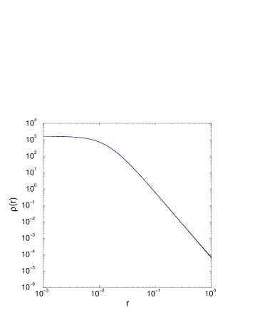
Figure 9: At $T=T_{c}=1/4$, and when the central density has reached the value $\rho(0,t)\approx 1644.8...=\frac{a(t)+1}{\pi}$ ($a(t)\approx 5166.3...$), we have plotted the result of the numerical calculation compared to our exact scaling form $\rho(r,t)=\frac{a(t)+1}{\pi}(1+a(t)r^{2})^{-2}$ obtained in Eq. (129). The two curves are indistinguishable as the relative error is, as predicted, of order $a^{-1}\sim 10^{-4}$. Note finally that for this range of density, the density contrast is huge, of order $10^{7}$.

Integrating Eq. (135) for large time, we get the exact asymptotic expansion for large time

(136) $$a(t)=\exp\left(\frac{5}{2}+\sqrt{2t}\right)\left[1+O(t^{-1/2}\ln t)\right].$$

For $t\rightarrow+\infty$, the central density diverges like $a(t)$ and the core radius goes to zero like $a(t)^{-1/2}$. In addition, the scaling solution (129) at $T=T_{c}$ goes to a Dirac peak containing the whole mass (see Eq. (41)), as the decay exponent of the scaling function is 4, which is strictly greater than 2.

Figure 10: We plot $a(da/dt)^{-1}$ as a function of $\ln a$, which is predicted to behave as $a(da/dt)^{-1}\sim\ln a-5/2+O([\ln a]^{-1})$ (see Eq. (135)). Even for the moderate range of accessible densities ($a_{\rm max}\sim 5166$), we clearly find that the numerical result evolves toward the theoretical asymptotic (dashed line).

4.3 Collapse for $T<T_{c}$

For $D=2$, the scaling equation associated to Eq. (85) does not display any physical solution when numerically solved. In this section, we thus present a special treatment adapted to this case. The principal difference with other dimensions is the divergence of the central density at $T_{c}$, and the occurrence of a scaling solution at this temperature.

Strictly below $T_{c}$, we expect a finite time collapse. Close to the center, the solution takes the form

(137) $$M(u,t)\approx 4T\frac{a(t)u}{1+a(t)u},$$

where again the left-hand side of Eq. (124) is negligible compared to each term on the right-hand side. We thus look for a solution of the type

(138) $$M(u,t)=4T\frac{a(t)u}{1+a(t)u}+h(u,t),$$

where $h$ is now of order $O(1)$ as it contains a finite fraction of the total mass, since the first term contains a mass of order $4T<1$. Inserting this ansatz in the dynamical equation Eq. (124), we obtain

(139) $$\frac{1}{4T}\frac{\partial h}{\partial t}+\frac{da}{dt}\frac{u}{(1+au)^{2}}=u\frac{\partial^{2}h}{\partial u^{2}}+2\frac{\partial}{\partial u}\left(\frac{au}{1+au}h\right)+2h\frac{\partial h}{\partial u}.$$

One can look for a scaling solution of the type

(140) $$h(u,t)=a^{\gamma-1}H(au),{\rm\ with\ }H(v)\sim cv^{1-\gamma},{\rm\ when\ }v\to+\infty,$$

so that the mass included in this scaling profile $h(1,t)=c=O(1)$. With this definition, the density profile decays for large distance as $\rho\sim r^{-\alpha}$, with $\alpha=2\gamma$. Inserting this ansatz in Eq. (139), we obtain

(141) $$\left[\frac{1}{4T}\left(vH^{\prime}+(\gamma-1)H\right)+a^{1-\gamma}\frac{v}{(1+v)^{2}}\right]\frac{da}{dt}a^{-2}=vH^{\prime\prime}+2\left(\frac{v}{1+v}H\right)^{\prime}+2a^{\gamma-1}HH^{\prime},$$

where derivatives are with respect to the variable $v$. We are free to choose $a(t)=\pi\rho(0,t)/(4T)$, so that $H^{\prime}(0)=H(0)=0$. For small $v$, Eq. (141) leads to

(142) $$\frac{da}{dt}=H^{\prime\prime}(0)a^{\gamma+1}.$$

Eq. (141) has a global scaling solution only for $\gamma=1$. However, we know that in this case the scaling equation obtained by setting $\gamma=1$ does not display any physical solution. Thus, we conclude that there is no scaling solution obtained by imposing that all terms in Eq. (141) scale the same way. However, as we will see in the section devoted to numerical simulations, the direct simulation of Eq. (124) seems to display a scaling solution with $\gamma\approx 0.6-0.7$ for numerically accessible densities. Strictly speaking, this is totally excluded by the above equation, except if one allows $\gamma$ to very slowly depend on the density or $a$. For a given $a$, we thus want to solve Eq. (141), where the boundary conditions will ultimately select the effective value of $\gamma$, and that of ${da}/{dt}$. More precisely, once we impose $H^{\prime}(0)=H(0)=0$, and the condition of Eq. (142), we end up with a shooting problem for $H^{\prime\prime}(0)$ and $\gamma$. For large $a$, and $v\ll a$, it is clear that the non linear term of the right-hand side of Eq. (141) becomes irrelevant, and we drop it from now on.

In order to understand the origin of this shooting problem, and to obtain an accurate estimate of $\gamma$, let us solve Eq. (141) in the limit of very large $a$, in the range $1\ll v\ll a$. In this regime, Eq. (141) simplifies to the following equation

(143) $$\left[\frac{1}{4T}\left(vH^{\prime}+(\gamma-1)H\right)+a^{1-\gamma}v^{-1}\right]\omega=vH^{\prime\prime}+2H^{\prime},$$

where

(144) $$\omega=\frac{da}{dt}a^{-2}=H^{\prime\prime}(0)a^{\gamma-1}.$$

Let us now multiply this equation by $v^{\gamma-2}$ and integrate the resulting equation. After elementary manipulations, we obtain

(145) $$H^{\prime}+\left[\frac{3-\gamma}{v}-\frac{\omega}{4T}\right]H=-\frac{\omega c}{4T}v^{1-\gamma}-\frac{\omega a^{1-\gamma}}{2-\gamma}v^{-1}+(2-\gamma)(3-\gamma)v^{1-\gamma}\int_{v}^{+\infty}w^{\gamma-3}H(w)\,dw,$$

where $c\sim O(1)$, which has been defined in Eq. (140), appears here as an integration constant. Then, one can integrate this differential equation which leads to the following self-consistent relation for $H$:

(146) $$H(v)=v^{\gamma-3}\exp\left(\frac{\omega v}{4T}\right)\int_{v}^{+\infty}w^{3-\gamma}\exp\left(-\frac{\omega w}{4T}\right)F(w)\,dw,$$

where $F$ is defined as the opposite of the right-hand side of Eq. (145):

(147) $$F(v)=\frac{\omega c}{4T}v^{1-\gamma}+\frac{\omega a^{1-\gamma}}{2-\gamma}v^{-1}-(2-\gamma)(3-\gamma)v^{1-\gamma}\int_{v}^{+\infty}w^{\gamma-3}H(w)\,dw.$$

Eq. (143) implies that $H(v)\sim\ln v$, when $v\to 0$ (of course, this apparent divergence does not occur in the full dynamical equation Eq. (141)). Considering the prefactor $v^{\gamma-3}$ in Eq. (146), this behavior can be obtained if and only if

(148) $$\int_{0}^{+\infty}w^{3-\gamma}\exp\left(-\frac{\omega w}{4T}\right)F(w)\,dw=0.$$

As $\omega$ is expected to go to zero for large $a$ as $\gamma<1$ (see Eq. (144)), the dominant contribution of the integral of the third term in the definition of $F$ comes from the large $w$ region, for which $H$ can be replaced by its asymptotic form. Hence, defining $\Gamma(x)=\int_{0}^{+\infty}w^{x}\exp(-w)\,dw$ and $\varepsilon=1-\gamma$, and using Eq. (144), the condition expressed in Eq. (148) can be rewritten

(149) $$c=\frac{\Gamma(1+\varepsilon)}{\varepsilon(1+\varepsilon)^{2}\Gamma(1+2\varepsilon)}H^{\prime\prime}(0)\left(\frac{H^{\prime\prime}(0)}{4T}\right)^{\varepsilon}a^{-\varepsilon^{2}}.$$

As $c$ is of order $O(1)$, we find that $\varepsilon\to 0$ as $a\to+\infty$. More precisely, in this limit, $\varepsilon$ is the solution of the following implicit equation

(150) $$\varepsilon=\sqrt{\frac{\ln(K/\varepsilon)}{\ln a}},$$

where $K=H^{\prime\prime}(0)/c+O(\varepsilon)$. Finally, we obtain

(151) $$\varepsilon=1-\gamma=\sqrt{\frac{\ln\ln a}{2\ln a}}\left(1+O([\ln\ln a]^{-1})\right).$$

In conclusion, although the solution is not strictly speaking a true scaling solution, the explicit dependence of $\gamma$ on $a$ is so weak that an apparent scaling should be seen with an effective $\gamma$ almost constant for a wide range of values of $a$. Hence, the total density profile is the sum of the scaling profile obtained at $T_{c}$ with a $T/T_{c}$ weight (behaving as a Dirac peak of weight $T/T_{c}$, at $t=t_{coll}$) and of a pseudo-scaling solution associated to an effective scaling exponent slowly converging to $\alpha=2$.

Let us illustrate quantitatively the time dependence of $\alpha=2\gamma$. For example, taking arbitrarily $K=1$ (the dependence on $K$ is weak and vanishes for large $a$), Eq. (150) and Eq. (151) respectively lead to $\gamma(a=10^{3})=0.624...$ and $\gamma(a=10^{3})=0.626...$, and to $\gamma(a=10^{5})=0.684...$ and $\gamma(a=10^{5})=0.674...$ (note that the error between the asymptotic expansion of Eq. (151) and the implicit expression first grows before slowly decaying for $a\gg 10^{12}$ !). Finally, for the maximum value of $a$ accessible numerically of order $a\sim 10^{4}$, we expect to observe an apparent scaling solution with $\gamma\approx 0.65$, or $\alpha=2\gamma\approx 1.3$.

Figure 11: At $T=T_{c}/2=1/8$, we have extracted the next correction to scaling $\rho_{\rm cor}=\rho-4T\rho_{T=T_{c}}$, where $\rho_{T=T_{c}}$ is defined in Eq. (129). We have then plotted $\rho_{\rm cor}(r,t)/\rho_{\rm cor}(r_{\rm max}(t),t)$ as a function of $x=r/r_{\rm max}(t)$, where $r_{\rm max}(t)$ is defined as the location of the maximum of $\rho_{\rm cor}(r,t)$. Consistently with the apparent scaling observed, we found $r_{\rm max}^{-1}(t)\sim\sqrt{a}\sim\sqrt{\rho_{\rm cor}(r_{\rm max}(t),t)}$. For $a=2^{n-1}\times 100$ ($n=1,...,8$), we have obtained a convincing data collapse associated to $\alpha=2\gamma\approx 1.3$, in agreement with the theoretical estimate of $\gamma$, in this range of $a$.

4.4 Numerical simulations

In this subsection, we present numerical simulations concerning the two-dimensional case. Indeed, the three-dimensional case has been extensively studied in [1]. It has been shown that the scaling function as well as the corrections to scaling (which have been calculated for the canonical ensemble in [1]) are perfectly described by the theory. In addition, as the system behaves qualitatively the same for any dimension $D>2$ in both thermodynamical ensembles, we have decided to focus on the numerical study of the $D=2$ case, which displays some very rich behaviors, as exemplified in the present section.

We consider the system in the canonical ensemble, as the gravitational collapse does not occur in the microcanonical ensemble. In Fig. 9, we show the scaling function at $T_{c}$, as given by Eq. (129), finding a perfect agreement. In Fig. 10, we also display $a(da/dt)^{-1}$ as a function of $\ln a$, and find an asymptotic behavior fully compatible with that given by Eq. (135).

Below $T_{c}$, and in the accessible range of $a$ (up to $a\sim 10^{5}$), we find an apparent scaling regime with $\alpha=2\gamma\approx 1.3$, as predicted in Sec. 4.3. This is illustrated in Fig. 11, for $T=T_{c}/2=1/8$. Note that the effective $\gamma$ or $\alpha$ can also be extracted from the time evolution of $a(t)$ or the central density (see Eq. (142)). In Fig. 12, we show that this way of measuring $\gamma$ is fully compatible with the value of the effective exponents $\alpha=2\gamma\approx 1.3$

Figure 12: We plot $a^{-1}(da/dt)\sim a^{\gamma}$ as a function of $a$, in order to extract the effective value of $\gamma$ directly from the time evolution of the central density. We find that the effective $\gamma$ is slowly growing with time, as predicted, and is of order $\gamma=\alpha/2\approx 0.65$ (the dashed line has a slope equal to 0.65), which is fully compatible with the value extracted from Fig. 11, and the value expected from Eq. (150) in this range of $a$.

5 The one dimensional case

When an equilibrium state exists, there is little hope to be able to solve the full Smoluchowski-Poisson system analytically in order to study the relaxation towards equilibrium. We shall consider a simpler problem in which a test particle evolves in a medium of field particles at statistical equilibrium (thermal bath approximation). The particles are assumed to create a stationary potential $\Phi_{eq}({\bf r})$ which induces a drift of the test particle along the gradient of $\Phi_{eq}$. In addition, the test particle is assumed to experience a diffusion process. If $\rho$ denotes the density probability of finding the test particle in ${\bf r}$ at time $t$, we expect the evolution of $\rho$ to be determined by a Smoluchowski equation of the form

(152) $${\partial\rho\over\partial t}=\nabla(T\nabla\rho+\rho\nabla\Phi_{eq}),$$

where $\Phi_{eq}({\bf r})$ is solution of the Boltzmann-Poisson equation (11). This means that we replace the true potential by its equilibrium value but still allow the density $\rho$ to vary with time. As we shall see, it is possible to solve the Smoluchowski equation (152) analytically in $D=1$ by using an analogy with a problem of quantum mechanics. An equation of the form (152) has been proposed in Refs. [27, 25] to model the motion of a test vortex in a bath of field vortices at statistical equilibrium. In that context, Eq. (152) can be formally derived from the $N$-body Liouville equation of the system by using projection operator technics.

It is well-known that a Fokker-Planck equation like Eq. (152) can be formally transformed into a Schrödinger equation with imaginary time. Indeed, performing the change of variable

(153) $$\rho=\psi e^{-{1\over 2T}\Phi_{eq}},$$

we find that the evolution of $\psi$ is determined by an equation of the form

(154) $${\partial\psi\over\partial t}=T\Delta\psi+\biggl{(}{1\over 2}\Delta\Phi_{eq}-{1\over 4T}(\nabla\Phi_{eq})^{2}\biggr{)}\psi.$$

This can be written as a Schrödinger-type equation

(155) $${\partial\psi\over\partial t}=T\Delta\psi-V({\bf r})\psi,$$

with a potential $V({\bf r})=-{1\over 2}\Delta\Phi_{eq}+{1\over 4T}(\nabla\Phi_{eq})^{2}$. So far, this transformation is general. If we now consider the one-dimensional case, the Boltzmann-Poisson equation (152) can be solved analytically and the potential $V(r)$ determined explicitly. Introducing the notations $\xi=\alpha r/\sqrt{2}R$ and $\tau=\alpha^{2}Tt/2R^{2}$ and using Eq. (24) we can rewrite Eq. (154) in the form

(156) $${\partial\psi\over\partial\tau}=\Delta\psi+\biggl{(}{2\over\cosh^{2}\xi}-1\biggr{)}\psi.$$

A separation of the variables can be effected by the substitution

(157) $$\psi(\xi,t)=\phi(\xi)e^{-\lambda t}\qquad(\lambda\geq 0),$$

where $\phi$ is solution of the ordinary differential equation

(158) $${d^{2}\phi\over d\xi^{2}}+2\biggl{(}E+{1\over\cosh^{2}\xi}\biggr{)}\phi=0,$$

where we have set $\lambda-1=2E$. The solutions of this Schrödinger equation are described in detail in Ref. [28]. The spectrum of positive energies is continuous. The spectrum of negative energies is discrete and reduces to $E_{0}=-1/2$ (fundamental state). The first excited state in the continuum is $E_{1}=0$. We can check that the corresponding eigenfunctions are $\phi_{0}=1/\cosh\xi$ and $\phi_{1}=\tanh\xi$. In order to obtain the qualitative behavior of the time dependent solution of Eq. (152), we neglect the contribution from the continuum states with $E>0$, only keeping the $E=-1/2$ and $E=0$ eigenstates.

Within this approximation and for sufficiently large times, we obtain

(159) $$\psi(\xi,\tau)={A\over\cosh\xi}+B\tanh\xi\ e^{-\tau},\qquad(\tau\rightarrow+\infty).$$

where $A$ and $B$ are constant. Returning to original variables, we get

(160) $$\rho(r,t)=\rho_{eq}(r)\biggl{\{}1+C\sinh\Bigl{(}{\alpha r\over\sqrt{2}R}\Bigr{)}e^{-{\alpha^{2}T\over 2R^{2}}t}+...\biggr{\}},$$

where $\rho_{eq}$ is given by Eq. (43) and $C=B/A$ is a constant. We find that the relaxation time is given by $t_{relax}=2R^{2}/\alpha^{2}T$.

6 Conclusion

In this paper, we have studied the Boltzmann-Poisson equation and the Smoluchowski-Poisson system in various dimensions of space. Our study shows in particular how the nature of the problem changes as we pass from $D=3$ to $D=2$. We showed that the dimension $D=2$ is critical in the sense that the results obtained for $D>2$ diverge if they are naively extrapolated to $D=2$. On a physical point of view, the two-dimensional problem differs from the $D>2$ case in two respects: in the 2D case, the central density of the equilibrium state is infinite at the critical temperature $T_{c}$ while it is finite at $T_{c}$ in higher dimensions. On the other hand, in $D=2$, the self-similar collapse results in a Dirac peak which contains a finite fraction of mass, while for $D>2$, the mass contained in the core tends to zero at the collapse time (but a Dirac peak is always formed in the canonical ensemble after $t_{coll}$ as discussed in Appendix B). We have also evidenced another characteristic dimension $D=10$ at which the nature of the problem changes. For $D\geq 10$ the classical spiral characterizing isothermal spheres in the physical three-dimensional space disappears. However, since the points in the spiral correspond to unstable states, that are therefore unphysical, this transition at $D=10$ is not so critical and indeed the nature of the self-similar collapse does not show any transition at that dimension. It is interesting to note that the dependance of the phase diagram in the $(E,T)$ and $(u,v)$ planes with the dimension of space $D$ shows some resemblance with the dependance of the phase diagram of confined polytropic spheres with the index $n$ of the polytrope [29]. An extension of our study would be to relax the high friction limit and consider solutions of the Kramers-Poisson system and other relaxation equations described in Ref. [2]. These equations are expected to display qualitatively similar behaviors than those described here (i.e. gravitational collapse, finite time singularity, self-similar solutions,…) but their study appears to be of considerable difficulty since we now need to consider the evolution of the system in phase space. We hope to come to that problem in future publications.

Appendix A Absence of global maximum of free energy in $D=2$ for $T<T_{c}=GM/4$

We give a proof similar to the one given in Ref. [18] for $D=3$. In two dimensions, we consider a homogeneous disk of mass $M$ and radius $a$ at temperature $T$. It is easy to show that the total energy (8) of this disk is

(161) $$E=MT+{1\over 2}GM^{2}\Bigl{(}\ln a-{1\over 4}\Bigr{)},$$

with the convention $\Phi\sim GM\ln r$ at large distances. According to Eqs. (6) and (9), its free energy reads

(162) $$J=M\ln T-M\ln\biggl{(}{M\over\pi a^{2}}\biggr{)}-M-{GM^{2}\over 2T}\Bigl{(}\ln a-{1\over 4}\Bigr{)}.$$

For $a\rightarrow 0$, the free energy behaves like

(163) $$J\sim 2M\biggl{(}1-{GM\over 4T}\biggr{)}\ln a.$$

Therefore, if $T<T_{c}=GM/4$ the free energy goes to $+\infty$ when we contract the system to a point. This is sufficient to prove the absence of a global maximum of free energy below $T_{c}$. This also shows the natural tendency (in a thermodynamical sense) of a canonical self-gravitating system to collapse to a Dirac peak for $T<T_{c}$.

Appendix B The case of cold systems ($T=0$)

For $T=0$, Eq. (88) reduces to

(164) $$\frac{\partial s}{\partial t}=\left(r\frac{\partial s}{\partial r}+ds\right)s.$$

Looking for a self-similar solution of the form (92) and imposing the conditions (94) and (96), we find that the scaling profile satisfies

(165) $$xS^{\prime}+\alpha S=\left(xS^{\prime}+DS\right)S.$$

Of course, for $T=0$, the exponent $\alpha$ cannot be determined on dimensional grounds, as the definition $r_{0}=\sqrt{T/\rho_{0}}$ is not relevant anymore. As we will see, $\alpha$ will be determined by imposing that the scaling solution is analytic. Eq. (165) can be readily solved leading to the following implicit equation for $S$:

(166) $$\left(\frac{\alpha}{D}-S(x)\right)^{1-\frac{\alpha}{D}}=Kx^{\alpha}S(x),$$

where $K$ is an integration constant. Now, from the definition of $S$, we expect a small $x$ expansion of the form $S(x)=S(0)+\frac{1}{2}S^{\prime\prime}(0)x^{2}+O(x^{4})$, which first implies that

(167) $$S(0)=\frac{\alpha}{D},$$

and that $(x^{2})^{1-\alpha/D}\sim x^{\alpha}$, which finally leads to

(168) $$\alpha=\frac{2D}{D+2}\qquad{\rm and}\qquad K={D+2\over 2}\biggl{(}{1\over 2}|S^{\prime\prime}(0)|\biggr{)}^{D\over D+2}.$$

In terms of the scaling function $g(x)$ associated to the mass profile, Eq. (166) can be rewritten

(169) $$g(x)=\frac{2x^{D}}{D+2}-\frac{|S^{\prime\prime}(0)|}{2}\left[\frac{D+2}{2}g(x)\right]^{\frac{D+2}{D}},$$

where $S^{\prime\prime}(0)<0$ is arbitrary. This leads to the exact large $x$ asymptotic behavior

(170) $$g(x)\sim\frac{2}{D+2}\left(\frac{4}{(D+2)|S^{\prime\prime}(0)|}\right)^{\frac{D}{D+2}}x^{\frac{D^{2}}{D+2}}.$$

Moreover, using Eq. (96) and (167), we get the exact universal asymptotic behavior of the central density

(171) $$\rho(0,t)\sim S_{D}^{-1}(t_{coll}-t)^{-1},$$

Finally, we note that the implicit equation (169) can be written as a parametric set of equations

(172) $$g(y)=\frac{2}{D+2}y,\qquad x(y)=\left[y+\frac{D+2}{4}|S^{\prime\prime}(0)|y^{\frac{D+2}{D}}\right]^{\frac{1}{D}}.$$

These results can be obtained by a different, more physical, method. We have indicated in Ref. [1] that, for $T=0$, the particles have a deterministic motion with equation

(173) $${d{\bf r}\over dt}={\bf u}=-\nabla\Phi.$$

For a spherically symmetrical system, this can be rewritten

(174) $${dr\over dt}=-{M(r,t)\over r^{D-1}},$$

where $M(r,t)$ is the mass within $r$. If $a$ denotes the initial position of the particle located at $r$ at time $t$, we have

(175) $$M(r,t)=M(a,0),$$

so Eq. (174) can be integrated explicitly in

(176) $$r^{D}=a^{D}-DM(a,0)t.$$

If $M(a,0)$ behaves like

(177) $$M(a,0)=A(a^{D}-Ba^{D+2})+...,$$

close to the origin (which is a regular expansion), then

(178) $$M(r,t)=Aa^{D}(1-Ba^{2}),\qquad{\rm with}\qquad r^{D}=(1-DAt)a^{D}+DABa^{D+2}t.$$

Introducing the collapse time $t_{coll}=1/DA$ and considering the limit $t\rightarrow t_{coll}$, we obtain

(179) $$M(r,t)={a^{D}\over Dt_{coll}},\qquad{\rm with}\qquad r^{D}={1\over t_{coll}}(t_{coll}-t)a^{D}+Ba^{D+2}.$$

Introducing the scaling variables

(180) $$x={r\over(t_{coll}-t)^{D+2\over 2D}},\qquad y={1\over t_{coll}}\biggl{[}{a\over(t_{coll}-t)^{1/2}}\biggr{]}^{D},$$

we can put the solution in a parametric form

(181) $$M(r,t)={1\over D}(t_{coll}-t)^{D/2}y,\qquad{\rm with}\qquad x=(y+Cy^{D+2\over D})^{1\over D},$$

where $C$ is a constant. At the collapse time $t=t_{coll}$,

(182) $$M(r,t=t_{coll})={1\over DC^{D\over D+2}}r^{D^{2}\over D+2},\qquad\rho(r,t=t_{coll})={D\over(D+2)S_{D}C^{D\over D+2}}r^{-{2D\over D+2}}.$$

These results are of course equivalent to those obtained previously.

We can now use this method to study the evolution of the system for $t>t_{coll}$ (post-collapse solution). For $t=t_{coll}+\delta t$, according to Eqs. (176) and (182), the mass contained inside the sphere of radius $a_{coll}=C^{-1/2}\delta t^{\frac{D+2}{2D}}$ at $t=t_{coll}$ has collapsed at $r=0$, resulting in a Dirac peak of weight

(183) $$M(0,t)={1\over DC^{D/2}}(t-t_{coll})^{D/2}.$$

Note that in a bounded domain the final collapse to a central Dirac peak containing the whole mass occurs in a finite time after $t_{coll}$. For $r>0$ (associated to $a>a_{coll}$), one has

(184) $$M(r,t)=M(0,t)+{1\over DC^{D\over D+2}}\left(a^{D^{2}\over D+2}-a_{coll}^{D^{2}\over D+2}\right),$$

(185) $$r^{D}=a^{D}\left(1-\left(\frac{a_{coll}}{a}\right)^{\frac{2D}{D+2}}\right).$$

Introducing the scaling variables

(186) $$x={r\over a_{coll}},\qquad y=\left(\frac{a}{a_{coll}}\right)^{\frac{D^{2}}{D+2}}-1,$$

we obtain

(187) $$M(r,t)=M(0,t)(1+y),\qquad{\rm with}\qquad x=(1+y)^{\frac{D^{2}}{D+2}}\left(1-(1+y)^{-{2\over D}}\right)^{1\over D}.$$

Subtracting the Dirac peak at $r=0$, and considering $x\ll 1$, for which $y\sim\frac{D}{2}x^{D}$, we find that the leading contribution to the mass profile for small $r$ is

(188) $$M(r,t)_{>}\approx\frac{r^{D}}{2\delta t}.$$

Hence the density profile does not diverge at $r=0^{+}$ for $t>t_{coll}$. Instead, the density approaches the constant value

(189) $$\rho(0+,t)=\frac{D}{2S_{D}\delta t},$$

which decreases with time. The density profile is thus depleted on a scale $r\sim a_{coll}\sim\delta t^{\frac{D+2}{2D}}$, which increases with time. For $r\gg a_{coll}$, the density profile remains essentially unaffected.

In principle, the same phenomenon arises for any $0<T<T_{c}$: the density profile obtained at $t_{coll}$ ultimately collapses into a central Dirac peak at a time $t_{*}>t_{coll}$. This solves the apparent paradox that the solution at $t=t_{coll}$ has a vanishing central mass and a finite free energy [1]. In fact, if we allow singular profiles to develop, the evolution continues for $t>t_{coll}$ and the Dirac peak with infinite free energy (predicted by statistical mechanics [14]) is formed during the post collapse regime of our Brownian model . In practice, degeneracy effects (of quantum or dynamical origin) lead to a finite small core of finite density, controlled by the maximum allowed degeneracy [30].

References

- [1] P.H. Chavanis, C. Rosier and C. Sire, “Thermodynamics of self-gravitating systems”, submitted to Phys. Rev. E (2002) [cond-mat/0107345].
- [2] P.H. Chavanis, J. Sommeria and R. Robert, “Statistical mechanics of two-dimensional vortices and collisionless stellar systems”, Astrophys. J. 471, 385 (1996).
- [3] T. Padmanabhan, “Statistical mechanics of gravitating systems”, Phys. Rep. 188, 285 (1990).
- [4] J. Katz and D. Lynden-Bell, “The gravothermal instability in two dimensions”, Mon. Not. R. astr. Soc. 184, 709 (1978).
- [5] A.M. Polyakov, Phys. Lett. 103B, 207 (1981).
- [6] M.E. Cates, Phys. Lett. 251B, 553 (1990).
- [7] D. Carpentier and P. Le Doussal, “Glass transition of a particle in a random potential, front selection in nonlinear renormalization group, and entropic phenomena in Liouville and sinh-Gordon models” Phys. Rev. E 63, 026110 (2001).
- [8] L. Onsager, “Statistical hydrodynamics”, Nuovo Cimento Suppl. 6, 279 (1949).
- [9] J.D. Murray, Mathematical Biology (Springer, 1991).
- [10] C. Rosier, “Problème de Cauchy pour une équation parabolique modélisant la relaxation des systèmes stellaires auto-gravitants”, C. R. Acad. Sci. Paris, Série I (2001).
- [11] P. Biler, P. Laurençot and T. Nadzieja, “Global and exploding solutions in a model of self-gravitating systems”, preprint.
- [12] G. Joyce and D. Montgomery, “Negative temperature states for the two-dimensional guiding-center plasma”, J. Plasma Physics 10, 107 (1973).
- [13] P.H. Chavanis and J. Sommeria, “Classification of self-organized vortices in two-dimensional turbulence: the case of a bounded domain” J. Fluid Mech. 314, 267 (1996).
- [14] M. Kiessling, “On the equilibrium statistical mechanics of isothermal classical selfgravitating matter”, J. Stat. Phys. 55, 203 (1989).
- [15] J.J. Aly, “Thermodynamics of a two-dimensional self-gravitating system”, Phys. Rev. E 49, 3771 (1994).
- [16] V.A. Antonov, Vest. Leningr. Gos. Univ. 7, 135 (1962).
- [17] T. Padmanabhan, “Antonov instability and the gravothermal catastrophe-revisited”, Astrophys. J. Supp. 71, 651 (1989).
- [18] P.H. Chavanis, “Gravitational instability of finite isothermal spheres”, Astron. Astrophys. 381, 340 (2002).
- [19] D. Lynden-Bell and R. Wood, “The gravothermal catastrophe in isothermal spheres and the onset of red-giants structure for stellar systems”, Mon. Not. R. astr. Soc. 138, 495 (1968).
- [20] J. Katz, “On the number of unstable modes of an equilibrium”, Mon. Not. R. astr. Soc. 183, 765 (1978).
- [21] S. Chandrasekhar, An introduction to the theory of stellar structure (Dover, 1939).
- [22] E. Caglioti, P.L. Lions, C. Marchioro, M. Pulvirenti, “A special class of stationary flows for two-dimensional Euler equations: a statistical mechanics description”, Commun. Math. Phys. 174, 229 (1995).
- [23] J. Binney and S. Tremaine, Galactic Dynamics (Princeton Series in Astrophysics, 1987).
- [24] H. Risken, The Fokker-Planck equation (Springer, 1989).
- [25] P.H. Chavanis “Kinetic theory of point vortices: diffusion coefficient and systematic drift”, Phys. Rev. E 64, 026309 (2001).
- [26] E. Abdalla and M.R.R Tabar, “Phase Transition in a Self-Gravitating Planar Gas”, Phys. Lett. B 440, 339 (1998).
- [27] P.H. Chavanis “Systematic drift experienced by a point vortex in two-dimensional turbulence”, Phys. Rev. E 58, R1199 (1998).
- [28] L. Landau and E. Lifschitz, Mécanique Quantique (Editions MIR, 1967).
- [29] P.H. Chavanis “Gravitational instability of polytropic spheres and generalized thermodynamics”, Astron. Astrophys., in press [astro-ph/0108378] (2002).
- [30] P.H. Chavanis, “Phase transitions in self-gravitating systems. Self-gravitating fermions and hard spheres models”, Phys. Rev. E, in press [cond-mat/0109294] (2002).