On apparent breaking the second law of thermodynamics in quantum transport studies

Abstract

We consider a model for stationary electronic transport through a one-dimensional chain of two leads attached to a perturbed central region (quantum dot) in the regime where the theory proposed recently by Čápek for a similar model of phonon transport predicts the striking phenomenon of a permanent current between the leads. This result based on a rigorous but asymptotic Davies theory is at variance with the zero current yielded by direct transport calculations which can be carried out in the present model. We find the permanent current to be within the error of the asymptotic expansion for finite couplings, and identify cancelling terms of the same order.

In recent years, the validity of the second law of thermodynamics has been questioned in several models Čápek (1998); Sheehan (1998); Nikulov (1999); Allahverdyan and Nieuwenhuizen (2000); Weiss (2000); Čápek (2002). In most of them the phenomenon of breaking the law was claimed to stem from the genuine quantum behaviour of the system considered, e.g. quantum entanglement between the system and bath. Several models support the idea that the quantum correlation features could be responsible for breaking the second law.

In spite of the seemingly academic nature of the models, had their predictions turned out to be true, it could have far reaching consequences in the practice. For example, in the rapidly developing field of nanotechnologies, the regimes of validity of the suggested models could be achieved with the present or soon incoming technology so that the predicted effects, if confirmed, could be used to supply power for the nano-machines Nikulov (1999). Thus, thorough experimental as well as further theoretical examination of this kind of models is a desirable task.

In this study, we consider a modified version of the model molecular ’demon’ operating between two reservoirs recently proposed by Čápek Čápek (2002). Namely, we study the electronic transport in a one-dimensional tight-binding chain the central part of which is considered as ’system’ and the rest of the chain forms two ’reservoirs’. While in a general fermionic case there might arise questions about the applicability of the standard projection techniques which assume separability of the system and bath Hilbert spaces this problem is harmless in our model since an exact mapping onto an excitonic chain using Jordan-Wigner transformation Tsvelik (1995) can be performed.

Then the standard techniques are fully justified and using the method of the modified Davies weak coupling theory from Čápek and Barvík (2001) and repeating the reasoning of Čápek (2002) we come to the result that a permanent stationary current (particle flow) between the two asymptotic parts of the chain is possible thus violating the second law. However, the present model can be solved explicitly in the full range of parameters, i.e. without the need to resort to any limit. The exact result contradicts the one obtained by the modified Davies weak coupling theory by Čápek. Now, let us consider the model in detail.

The Hamiltonian $H=H_{S}+H_{B}+H_{T}$ reads

$$H_{S} =\epsilon_{1}a^{{\dagger}}_{1}a_{1}+\epsilon_{2}a^{{\dagger}}_{2}a_{2}+J\,(a^{{\dagger}}_{1}a_{2}+a^{{\dagger}}_{2}a_{1})\ ,$$ (1)

$$H_{B} =\sum_{\alpha=1,2}\sum_{n=1}^{\infty}-\frac{\Delta}{2}(c^{{\dagger}}_{n+1\alpha}c_{n\alpha}+c^{{\dagger}}_{n\alpha}c_{n+1\alpha})$$

$$=\sum_{\bm{k},\alpha=1,2}\epsilon_{\bm{k}\alpha}\,c^{{\dagger}}_{\bm{k}\alpha}c_{\bm{k}\alpha}\ ,$$ (2)

$$H_{T} =\sum_{\alpha=1,2}V_{\alpha}(c^{{\dagger}}_{1\alpha}a_{\alpha}+a^{{\dagger}}_{\alpha}c_{1\alpha})$$

$$=\sum_{\bm{k},\alpha=1,2}(V_{\bm{k}\alpha}c^{{\dagger}}_{\bm{k}\alpha}a_{\alpha}+V^{*}_{\bm{k}\alpha}a^{{\dagger}}_{\alpha}c_{\bm{k}\alpha})\ ,$$ (3)

where $H_{S}$ denotes the part corresponding to the system, i.e. the quantum dot, $H_{B}$ describes the contacts (baths) and $H_{T}$ the tunneling between the respective contact and level of the dot. The second form of $H_{B},H_{T}$ is expressed in the eigenstates of the baths labeled by $\bm{k}$. All the creation and annihilation operators $a^{{\dagger}}_{\alpha},\ a_{\alpha},\ c^{{\dagger}}_{n\alpha},\ c_{n\alpha},(\text{or }c^{{\dagger}}_{\bm{k}\alpha},\ c_{\bm{k}\alpha})$ satisfy the anticommutation relations for the Fermi operators among themselves. It is assumed that $J,V_{\alpha},\text{ and }\Delta$ are real numbers.

In order to fully specify the problem we have to supply the initial conditions. Let us assume that before the initial time $t_{0}$ the system is decoupled from the contacts (i.e. $H_{T}$ is effectively equal to zero) and a particular contact is in the thermal equilibrium given by the values of the temperature $T_{\alpha}$ and electrochemical potential $\mu_{\alpha}$. The corresponding initial density matrix of the whole system is thus separable $\rho_{S+B}(t_{0})=\rho_{S}(t_{0})\otimes\rho_{B}^{\text{can}}$. At $t=t_{0}$ we switch on the tunneling interaction between the dot and the contacts and study the time evolution of the whole complex system dot plus baths.

The particle current into bath $\alpha,\ I_{\alpha}(t)$, is given by the time derivative of the particle number $N_{\alpha}=\sum_{\bm{k}}c^{{\dagger}}_{\bm{k}\alpha}c_{\bm{k}\alpha}=\sum_{n=1}^{\infty}c^{{\dagger}}_{n\alpha}c_{n\alpha}$ as ($\hbar=1$ in the whole paper)

$$\begin{split}I_{\alpha}(t)&=\langle\dot{N}_{\alpha}\rangle(t)=-i\langle[N_{\alpha},H]\rangle(t)\\ &=-i\sum_{\bm{k}}\bigl{(}V_{\bm{k}\alpha}\langle c^{{\dagger}}_{\bm{k}\alpha}a_{\alpha}\rangle(t)-V^{*}_{\bm{k}\alpha}\langle a^{{\dagger}}_{\alpha}c_{\bm{k}\alpha}\rangle(t)\bigr{)}\\ &=-iV_{\alpha}\bigl{(}\langle c^{{\dagger}}_{1\alpha}a_{\alpha}\rangle(t)-\langle a^{{\dagger}}_{\alpha}c_{1\alpha}\rangle(t)\bigr{)}\ ,\end{split}$$ (4)

where the mean value of an arbitrary operator $O$ is calculated by

$$\begin{split}\langle O\rangle(t)&=\mathrm{Tr}_{S+B}\bigl{(}\rho_{S+B}(t_{0})\,O(t)\bigr{)}=\mathrm{Tr}_{S+B}\bigl{(}\rho_{S+B}(t)\,O\bigr{)}\\ &=\mathrm{Tr}_{S+B}\bigl{(}\rho_{S+B}(t_{0})\,e^{iH(t-t_{0})}\,O\,e^{-iH(t-t_{0})}\bigr{)}\ .\end{split}$$ (5)

The particle current between any two adjacent sites is given by the analogy of the above formula with the creation and annihilation operators of the two sites Caroli et al. (1971).

In the stationary state the current does not depend on time and neither on the position of the sites between which it is evaluated (current is conserved and his divergence in the stationary state is thus zero). Therefore,

$$I^{\text{stat}}_{1}=-iJ\bigl{(}\langle a^{{\dagger}}_{1}a_{2}\rangle-\langle a^{{\dagger}}_{2}a_{1}\rangle\bigr{)}=-I_{2}^{\text{stat}}\ .$$ (6)

The solution of the model within the formalism of nonequilibrium Green functions is well known, see e.g. Caroli et al. (1971); Jauho et al. (1994); Haug and Jauho (1996). Therefore, we only briefly summarize the results here. If we define the one-particle density matrix of the dot by

$$\sigma_{\alpha\beta}(t)=\langle a^{{\dagger}}_{\beta}(t)a_{\alpha}(t)\rangle=-iG^{<}_{\alpha\beta}(t,t)$$ (7)

we get for the present model the result

$$\begin{split}\sigma(t)&=\mathbf{G}^{R}(t-t_{0})\cdot\sigma(t_{0})\cdot\mathbf{G}^{A}(t_{0}-t)\\ &+\int_{t_{0}}^{t}dt_{1}\,dt_{2}\mathbf{G}^{R}(t-t_{1})\cdot-i\mathbf{\Sigma}^{<}(t_{1}-t_{2})\cdot\mathbf{G}^{A}(t_{2}-t)\end{split}$$ (8)

where the retarded and advanced Green functions and the lesser selfenergy $\mathbf{G}^{R,A}(t),\mathbf{\Sigma}^{<}(t)$ are given as inverse Fourier transforms of

$$\mathbf{G}^{R,A}(\epsilon) =\begin{pmatrix}\epsilon-\epsilon_{1}-\Sigma^{R,A}_{1}(\epsilon)&-J\\ -J&\epsilon-\epsilon_{2}-\Sigma^{R,A}_{2}(\epsilon)\end{pmatrix}^{-1}$$ (9)

$$\mathbf{\Sigma}^{<}(\epsilon) =\begin{pmatrix}i\Gamma_{1}(\epsilon)f_{1}(\epsilon)&0\\ 0&i\Gamma_{2}(\epsilon)f_{2}(\epsilon)\end{pmatrix}$$ (10)

with

$$\Sigma^{R,A}_{\alpha}(\epsilon) =\Lambda_{\alpha}(\epsilon)\mp\frac{i}{2}\Gamma_{\alpha}(\epsilon)=\sum_{\bm{k}}\frac{|V_{\bm{k}\alpha}|^{2}}{\epsilon-\epsilon_{\bm{k}\alpha}\pm i\eta}$$

$$=V_{\alpha}^{2}g^{R,A}_{\alpha}(1,1;\,\epsilon)$$ (11)

$$f_{\alpha}(\epsilon) =\frac{1}{e^{\beta_{\alpha}(\epsilon-\mu_{\alpha})}+1}\ .$$ (12)

The Green functions $g^{R,A}_{\alpha}(1,1;\,\epsilon)$ are given by the matrix elements of the resolvents of the respective reservoirs and the parameters $\beta_{\alpha},\ \mu_{\alpha}$ denote their inverse temperature and electrochemical potential in the initial state.

In the limit $t_{0}\to-\infty$ which corresponds to the stationary state the first (initial conditions) term in (8) vanishes and the second one can be simplified by employing the Fourier transform yielding the final expression for the current

$$I_{1}=\int_{-\infty}^{\infty}\frac{d\epsilon}{2\pi}\,\Gamma_{1}(\epsilon)\Gamma_{2}(\epsilon)G^{R}_{12}(\epsilon)G^{A}_{21}(\epsilon)\bigl{(}f_{2}(\epsilon)-f_{1}(\epsilon)\bigr{)}\ .$$ (13)

One can immediately see that for the two bath being originally at the same temperature and electrochemical potential there is no stationary current between them. Also for different initial temperatures and/or electrochemical potentials the formula predicts correctly the stationary flow in the direction against the temperature and/or concentration gradient. This result is exact, i.e. it is valid for any values of the parameters in the Hamiltonian and, therefore, in the limit assumed by the modified Davies theory too.

Now, we want to express the current in terms of quantities employed in the modified Davies weak coupling formalism by Čápek. First, it should be noted that the presently considered model of a linear chain with at maximum nearest-neighbor interaction populated by fermions can be exactly mapped by the Jordan-Wigner transformation on the linear chain of Frenkel excitons which satisfy the Pauli commutation relations, i.e. anticommute on-site and commute at different sites, with the same form of the Hamiltonian expressed in terms of exciton operators, see Tsvelik (1995). Thus, the projection formalism used by Čápek can be safely used since no sign problem due to fermions appears. In the following, we solve by the projection method the corresponding exciton model but the results for the level occupations and the current are exactly equal to those of the fermion model.

Within the projection formalism only the reduced density matrix of the states of the dot is considered. The basis of the states in the Hilbert space of the dot corresponds to two excitonic levels and, thus, may be chosen to be $\mathcal{H}_{S}=\{|0\rangle\equiv|\mathrm{vac}\rangle,|1\rangle\equiv a^{{\dagger}}_{1}|0\rangle,|2\rangle\equiv a^{{\dagger}}_{2}|0\rangle,|3\rangle\equiv a^{{\dagger}}_{2}a^{{\dagger}}_{1}|0\rangle\}$. The reduced density matrix $\rho(t)$ with the matrix elements $\rho_{ij}(t)=\langle i|\rho(t)|j\rangle$ is given by

$$\begin{split}\rho(t)&=\mathrm{Tr}_{B}\bigl{(}\rho_{S+B}(t)\bigr{)}=\mathrm{Tr}_{B}\bigl{(}e^{-i\mathcal{L}(t-t_{0})}\rho_{S+B}(t_{0})\bigr{)}\\ &=\mathrm{Tr}_{B}\bigl{(}e^{-iH(t-t_{0})}\rho_{S+B}(t_{0})e^{iH(t-t_{0})}\bigr{)}\end{split}$$ (14)

with $\mathcal{L}\,\,\bullet=[H,\,\bullet]$ being the Liouville superoperator of the whole system. The relation between the one-fermion density matrix (7) and the above introduced exciton reduced density matrix (14) is as follows

$$\begin{split}\sigma_{11}(t)&=\rho_{11}(t)+\rho_{33}(t)\\ \sigma_{22}(t)&=\rho_{22}(t)+\rho_{33}(t)\\ \sigma_{12}(t)&=\rho_{12}(t)=\rho_{21}^{*}(t)=\sigma_{21}^{*}(t)\ .\end{split}$$ (15)

The modified Davies approach of Čápek and Barvík (2001) is valid in the limit $\lambda\to 0$ when the following scaling is performed $V_{\alpha}\to\lambda V_{\alpha}\text{ and }J\to\lambda^{2}J$. In this limit the reduced density matrix obeys the evolution equation

$$\frac{d\rho(t)}{dt}=-i\bigl{(}\mathcal{L}_{S}+\langle\mathcal{L}_{T}\rangle+i\mathcal{K}\bigr{)}\,\rho(t)$$ (16)

with the superoperator $\mathcal{L}_{S}$ corresponding to the dot Hamiltonian $H_{S}$ and

$$\langle\mathcal{L}_{T}\rangle\,\,\bullet =\mathrm{Tr}_{B}\bigl{(}[H_{T},\,\bullet\otimes\rho_{B}^{\mathrm{can}}]\bigr{)}$$ (17)

$$\mathcal{K}\,\,\bullet =\int_{0}^{\infty}d\tau\Bigl{\{}\mathrm{Tr}_{B}\bigl{(}(-i\mathcal{L}_{T}(\tau))(-i\mathcal{L}_{T})(\bullet\otimes\rho_{B}^{\mathrm{can}})\bigr{)}$$

$$\qquad\qquad\quad-\langle\mathcal{L}_{T}(\tau)\rangle\langle\mathcal{L}_{T}\rangle\,\bullet\Bigr{\}}$$ (18)

where $\mathcal{L}_{T}(\tau)=e^{i\mathcal{L}_{0}\tau}\mathcal{L}_{T}e^{-i\mathcal{L}_{0}\tau}$ corresponds to the tunneling Hamiltonian $H_{T}(\tau)=e^{iH_{0}\tau}H_{T}e^{-iH_{0}\tau}$ in a modified interaction picture with $H_{0}=H_{B}+H_{S}\bigl{|}_{J=0}$. It is this modification of the time dependence of the interaction superoperator entering the kernel $\mathcal{K}$ which distinguishes the Čápek’s approach from the original Davies weak coupling theory. To be explicit, the above equation for the elements we are interested in reads

$$\frac{d}{dt}\begin{pmatrix}\rho_{00}\\ \rho_{11}\\ \rho_{22}\\ \rho_{33}\\ \text{Re}\rho_{12}\\ \text{Im}\rho_{12}\end{pmatrix}=\begin{pmatrix}-(\Gamma_{1\uparrow}+\Gamma_{2\uparrow})&\Gamma_{1\downarrow}&\Gamma_{2\downarrow}&0&0&0\\ \Gamma_{1\uparrow}&-(\Gamma_{1\downarrow}+\Gamma_{2\uparrow})&0&\Gamma_{2\downarrow}&0&-2\lambda^{2}J\\ \Gamma_{2\uparrow}&0&-(\Gamma_{1\uparrow}+\Gamma_{2\downarrow})&\Gamma_{1\downarrow}&0&2\lambda^{2}J\\ 0&\Gamma_{2\uparrow}&\Gamma_{1\uparrow}&-(\Gamma_{1\downarrow}+\Gamma_{2\downarrow})&0&0\\ 0&0&0&0&-\frac{1}{2}(\Gamma_{1}+\Gamma_{2})&\epsilon_{1}^{\prime}-\epsilon_{2}^{\prime}\\ 0&\lambda^{2}J&-\lambda^{2}J&0&\epsilon_{2}^{\prime}-\epsilon_{1}^{\prime}&-\frac{1}{2}(\Gamma_{1}+\Gamma_{2})\end{pmatrix}\cdot\begin{pmatrix}\rho_{00}\\ \rho_{11}\\ \rho_{22}\\ \rho_{33}\\ \text{Re}\rho_{12}\\ \text{Im}\rho_{12}\end{pmatrix}$$ (19)

where

$$\begin{split}\Gamma_{\alpha\uparrow}&=2\pi\lambda^{2}\sum_{\bm{k}}|V_{\bm{k}\alpha}|^{2}f_{\alpha}(\epsilon_{\bm{k}\alpha})\,\delta(\epsilon_{\alpha}-\epsilon_{\bm{k}\alpha})\\ \Gamma_{\alpha\downarrow}&=2\pi\lambda^{2}\sum_{\bm{k}}|V_{\bm{k}\alpha}|^{2}\bigl{(}1-f_{\alpha}(\epsilon_{\bm{k}\alpha})\bigr{)}\,\delta(\epsilon_{\alpha}-\epsilon_{\bm{k}\alpha})\\ \Gamma_{\alpha}&=\Gamma_{\alpha\uparrow}+\Gamma_{\alpha\downarrow}=\lambda^{2}\Gamma_{\alpha}(\epsilon_{\alpha})\\ \epsilon_{\alpha}^{\prime}&=\epsilon_{\alpha}+\lambda^{2}\sum_{\bm{k}}\frac{|V_{\bm{k}\alpha}|^{2}}{\epsilon_{\alpha}-\epsilon_{\bm{k}\alpha}}=\epsilon_{\alpha}+\lambda^{2}\Lambda_{\alpha}(\epsilon_{\alpha})\ .\end{split}$$ (20)

The current from the site $2$ to $1$ which is in the stationary state equal to the current into the first reservoir is given by $I_{12}(t)=-2\lambda^{2}J\,\text{Im}\rho_{12}(t)$ and from the above equation can be found to be

$$I^{\text{stat}}_{1}=I_{12}^{\text{stat}}=\mathcal{T}_{12}(\rho_{22}-\rho_{11})=\mathcal{T}_{12}(\sigma_{22}-\sigma_{11})$$ (21)

with the transmission coefficient $\mathcal{T}_{12}$

$$\begin{split}\mathcal{T}_{12}&=2\pi\lambda^{4}\,J^{2}\frac{1}{2\pi}\frac{\Gamma_{1}+\Gamma_{2}}{\bigl{(}\epsilon_{1}^{\prime}-\epsilon_{2}^{\prime}\bigr{)}^{2}+\bigl{(}\frac{1}{2}(\Gamma_{1}+\Gamma_{2})\bigr{)}^{2}}\\ &=2\pi\lambda^{4}\,J^{2}\int_{-\infty}^{\infty}d\epsilon\frac{1}{2\pi}\frac{\Gamma_{1}}{\bigl{(}\epsilon-\epsilon_{1}^{\prime}\bigr{)}^{2}+\bigl{(}\frac{1}{2}\Gamma_{1}\bigr{)}^{2}}\\ &\qquad\qquad\qquad\quad\cdot\frac{1}{2\pi}\frac{\Gamma_{2}}{\bigl{(}\epsilon-\epsilon_{2}^{\prime}\bigr{)}^{2}+\bigl{(}\frac{1}{2}\Gamma_{2}\bigr{)}^{2}}\ .\end{split}$$ (22)

Since the current may be expressed in terms of occupation numbers $\sigma_{11},\ \sigma_{22}$ only we search for an equation equivalent to (19) for these quantities. Indeed, it is possible to find such an equation using the normalization condition $\mathrm{Tr}_{S}(\rho)=\sum_{i=0}^{3}\rho_{ii}=1$ and bearing in mind that $\sigma_{\alpha\alpha}=\rho_{\alpha\alpha}+\rho_{33}$. We may then write

$$\begin{pmatrix}\Gamma_{1}+\mathcal{T}_{12}&-\mathcal{T}_{12}\\ -\mathcal{T}_{12}&\Gamma_{2}+\mathcal{T}_{12}\end{pmatrix}\cdot\begin{pmatrix}\sigma_{11}\\ \sigma_{22}\end{pmatrix}=\begin{pmatrix}\Gamma_{1\uparrow}\\ \Gamma_{2\uparrow}\end{pmatrix}$$ (23)

with the result

$$\sigma_{11}-\sigma_{22}=\frac{f_{1}(\epsilon_{1})-f_{2}(\epsilon_{2})}{1+\mathcal{T}_{12}(\Gamma_{1}^{-1}+\Gamma_{2}^{-1})}\approx f_{1}(\epsilon_{1})-f_{2}(\epsilon_{2})\ .$$ (24)

We have used the fact that $\Gamma_{\alpha\uparrow}=f_{\alpha}(\epsilon_{\alpha})\Gamma_{\alpha}$ and omitted the higher orders terms in $J$ in the last step.

This result together with Eqs. (21), (22) predicts the striking phenomenon of spontaneous particle current between identical baths if $\epsilon_{1}\neq\epsilon_{2}$ in the same manner as Čápek obtained a nonzero energy flow in Čápek (2002). It is a remarkable fact that the result does not depend on the nature of the bath, i.e. the permanent current is obtained in analogous manner for the phononic bath considered by Čápek as well as for the excitonic (and thus also fermionic) bath in our case. The only point where the nature of the bath enters is the formula for the rates and energy renormalization (20). From the physical point of view this fact is fully plausible since for a generic bath only its temperature (and electrochemical potential) should matter in the thermodynamic predictions.

Now, we come to a contradiction since we know from the exact solution that there is in fact no such a permanent current. Where is the problem in the mathematical reasoning and what are its physical roots? We are going to answer these questions as follows. First, one should note that the stationary current $I^{\text{stat}}_{1}$ is proportional to $\lambda^{6}$ (the extra factor $\lambda^{2}$ comes from $\Gamma_{1}+\Gamma_{2}$). If we really performed the van Hove limit $t\to\lambda^{-2}t,\ \lambda\to 0$ in which the Davies theory is valid we would obtain the zero value of the stationary current.

As pointed out by Čápek in Čápek (2002), when studying a particular physical system, we cannot actually scale the interaction strengths to zero since the values are given constants for that system. At most, we could have a set of similar physical systems with different values of coupling constants which could be considered a series of the same system with the value of $\lambda$ being gradually scaled down to zero. Then, one expects that the Davies theory gives more and more precise predictions about the system’s time evolution.

This intuitive formulation has as its mathematical counterpart the relation

$$\lim_{\lambda\to 0}\ \sup_{0\leq\lambda^{2}t\leq a}||\rho^{\text{exact}}(t)-\rho^{\text{Davies}}(t)||=0\ ,\text{ for any finite $a$}$$ (25)

true both for the original and modified Davies theory Čápek and Barvík (2001) which implies an analogous statement for every matrix component of $\rho(t)$ and, in particular, for $\text{Im}\rho_{12}(t)$, too. However, this statement is in fact too weak to be of any practical use for finite $\lambda$’s, as it is asymptotic by nature.

We may obtain a more precise estimate about the order of the asymptotic contact if we make an additional assumption (not implied by the Davies theory) that the $\lambda$ asymptotics is regular. Then, we can pictorially show how the Davies statement is in practice realized. In Figs. 1, 2 there are depicted $\text{Im}\rho_{12}(t)$ for the exact and the Davies evolution, respectively, for our one-dimensional fermionic chain with $t_{0}=0,\ \Delta=1,\ T_{1}=T_{2}=0.1,\ \mu_{1}=\mu_{2}=0,\ \epsilon_{1}=-0.1,\ \epsilon_{2}=0.2,\ J=0.001,\ V_{1}=0.1,\ V_{2}=0.15,\ \rho_{00}(t_{0})=1\text{ (initially empty dot)}$ for $\lambda=1\text{ and }0.3$.

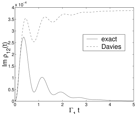
Figure 1: Comparison of the exact evolution of $\text{Im}\rho_{12}(t)$ with the modified Davies approximation due to Čápek. The value of $\lambda$ is $1.0$. For the rest of parameters see the text.

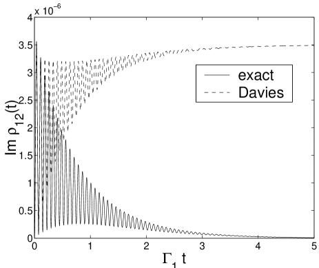
Figure 2: Comparison of the exact evolution of $\text{Im}\rho_{12}(t)$ with the modified Davies approximation due to Čápek for $\lambda=0.3$, the other parameters are given in the text.

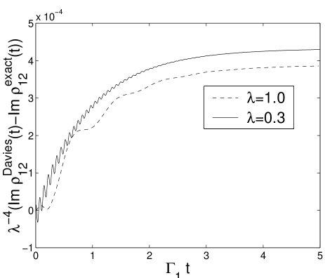
Figure 3: The difference between the approximate and exact evolution of the element $\text{Im}\rho_{12}(t)$ for two values of $\lambda$.

In Fig. 3 there is shown the scaled difference $\lambda^{-4}\text{Im}(\rho^{\text{Davies}}_{12}(t)-\rho^{\text{exact}}_{12}(t))$ for the two $\lambda$’s. This clearly shows that the difference between these two quantities for any finite scaled time goes to zero roughly as $\lambda^{4}$ in agreement with the Davies statement. Yet the exact result does not exhibit any permanent stationary current. Indeed, when one thoroughly inspects the Davies formula (25) one has to come to the result that it is fully consistent with the zero stationary current as illustrated by our pictures. On the other hand it does not exclude the possibility of a nonzero value in general which only means that its predictive power concerning this issue is essentially zero. The conclusion drawn by Čápek from it is doubtful since what he finds to be the stationary current breaking the second law of thermodynamics is of the same order in $\lambda$ as the terms neglected in a systematic Davies theory.

Now, let us discuss the physical mechanism of the above apparent paradox and the role of the quantum mechanics in it. As obvious from the above, the Davies theory neglects the higher order processes in $\lambda$. Actually, it can be considered as a sort of quasi-classical limit yielding the Pauli equation while omitting higher order quantum mechanical processes. Obviously, it does not take into account properly processes of direct coherent tunneling between the baths for finite $\lambda$. Most probably, just these higher order coherent processes exactly cancel the spurious stationary quasi-classical current as one can infer by a comparison of the exact transport formula (13) with the Davies one (21). Thus, referring to the conjectures mentioned in the introduction, for this particular model the coherent quantum mechanical features of the model prevent the second law from being violated rather than allowing it. It is interesting that an analogous discrepancy between the two approaches (reduced density matrix versus NGF) was reported by Wacker Wacker in a more complicated transport study.

To conclude, we have presented an exactly solvable model of quantum transport and used it to test the validity of the predictions by Čápek about the violation of the second thermodynamics law. We found, however, these predictions based on the Davies theory, rigorous in itself, as unwarranted. The point is that the predicted permanent current (or energy flow) is within the error of the asymptotic Davies theory for any finite coupling strength.

References

• Čápek (1998) V. Čápek, Phys. Rev. E 57, 3846 (1998).
• Sheehan (1998) D. P. Sheehan, Phys. Rev. E 57, 6660 (1998).
• Nikulov (1999) A. V. Nikulov, About perpetuum mobile without emotions (1999), eprint physics/9912022.
• Allahverdyan and Nieuwenhuizen (2000) A. E. Allahverdyan and T. M. Nieuwenhuizen, Phys. Rev. Lett. 85, 1799 (2000).
• Weiss (2000) P. Weiss, Science News 158, 234 (2000).
• Čápek (2002) V. Čápek, European Physical Journal B 25, 101 (2002), eprint cond-mat/0012056 v2.
• Tsvelik (1995) A. M. Tsvelik, Quantum Field Theory in Condensed Matter Physics (Cambridge University Press, 1995).
• Čápek and Barvík (2001) V. Čápek and I. Barvík, Physica A 294, 388 (2001).
• Caroli et al. (1971) C. Caroli, R. Combescot, P. Nozieres, and D. Saint-James, J. Phys. C: Solid St. Phys. 4, 916 (1971).
• Jauho et al. (1994) A.-P. Jauho, N. S. Wingreen, and Y. Meir, Phys. Rev. B 50, 5528 (1994).
• Haug and Jauho (1996) H. Haug and A.-P. Jauho, Quantum Kinetics in Transport and Optics of Semiconductors (Springer, 1996).
• (12) A. Wacker, Transport in nanostructures: A comparison between nonequilibrium Green functions and density matrices, to appear in Advances in Solid State Physics, ed. by B. Kramer (Springer 2001), eprint cond-mat/0105312.