Extended states in a one-dimensional generalized dimer model

Abstract

The transmission coefficient for one dimensional systems is given in terms of Chebyshev polynomials using the tight binding model. This result is applied to a system composed of two impurities located between $N$ sites of a host lattice. It is found that the system has extended states for several values of the energy. Analytical expressions are given for the impurity site energy in terms of the electron’s energy. The number of resonant states grow like the number of host sites between the impurities. This property makes the system interesting since it is a simple task to design a configuration with resonant energy very close to the Fermi level $E_{F}$.

Since the seminal paper of Anderson anderson , the problem of localization has been fundamental for the understanding of electronic transport in one dimensional disordered systems. The discovery of extended or delocalized states in systems with correlated disorder has renewed the interest in the transport properties of electrons for particular configurations of the lattice. Different types of systems [2-10] have been demonstrated to have extended states either with diagonal, or non-diagonal disorder or both.

One of the first systems studied was the so-called random dimer model (RDM) flores ; dunlap , in which a certain number of dimers (two adjacent impurities) were introduced randomly into the host lattice. Extended states with resonant energies equal to the site energy of the impurity were found.

In this paper, we describe a system consisting of two impurities hosted in a regular lattice and separated by $N$ lattice sites. This system is studied using the tight-binding Hamiltonian and the transfer matrix method. In addition, we use the Cayley-Hamilton theorem to express the transmission coefficient in terms of the Chebyshev polynomials of the second kind arfken . The transmission coefficient can be related to the conductance of the system through the Landauer formula landauer .

Consider a general $n\times n$ matrix $M$ whose characteristic equation can always be written as

$$\lambda^{n}=C_{n-1}\lambda^{n-1}+C_{n-2}\lambda^{n-2}+\cdots C_{0}.$$ (1)

We can write

$$\lambda^{n+1} = \lambda^{n}\lambda$$ (2)

$$= (C_{n-1}^{2}+C_{n-2})\lambda^{n-1}$$

$$+(C_{n-1}C_{n-2}+C_{n-3})\lambda^{n-2}+\cdots$$

and so on for higher powers of $\lambda$. In general the above equation will have the form

$$\lambda^{n+m}=p_{n+m-1}\lambda^{n-1}+p_{n+m-2}\lambda^{n-2}+\cdots+p_{m}\lambda^{0},$$ (3)

where the $p_{j}$ are polynomials in the trace and the minors of $M$. Now recall the Cayley-Hamilton theorem ma : if $p(\lambda)=0$ is the characteristic equation of $M$, then $p(M)=0$, that is, the matrix $M$ is also a “root” of the characteristic equation. The implication of this is that we can always write powers $M^{n+N}$ in terms of simpler expressions involving $M^{n-1}$ and the polynomials $p_{j}$.

In the case of a rank 2 transfer matrix with determinant equal to one, the characteristic equation is

$$\lambda^{2}=2x\lambda-1,$$ (4)

where $2x=\mbox{Tr}M$. It is easy to verify that higher powers of $\lambda$ are

$$\lambda^{3} = (4x^{2}-1)\lambda-2x,$$ (5)

$$\lambda^{4} = (8x^{3}-4x)\lambda-(4x^{2}-1),$$ (6)

$$\vdots \qquad\vdots$$ (7)

$$\lambda^{n} = p_{n-1}\lambda-p_{n-2},$$ (8)

and by virtue of the Cayley-Hamilton theorem, we can conclude

$$M^{n}=p_{n-1}M-p_{n-2}.$$ (9)

Note that the above formalism applies to a general matrix whose only requirement is to have a unit determinant. In the case of rank two matrices, the polynomials coincide with the second kind Chebyshev polynomials. The above results can be applied to either continuous pp1 ; sanchez as well to discrete type lattices.

In the following we consider the discrete one dimensional chain in the tight-binding approximation eco ; marder , for which we have the Hamiltonian

$$H=\sum_{n}\epsilon_{n}|n\rangle\langle n|+V\sum_{n}\left[|n\rangle\langle n+1|+|n\rangle\langle n-1|\right]$$ (10)

where $\epsilon$ is the site energy and $V$ is the hopping amplitude between nearest sites. The resultant Schrödinger equation is

$$i\dot{c}_{n}(t)=\epsilon_{n}c_{n}(t)+c_{n+1}(t)+c_{n-1}(t),$$ (11)

where $c_{n}(t)$ is the probability amplitude for an electron to be at site $n$. After the substitution $c_{n}(t)=C_{n}\exp(-iEt)$, where $E$ is the energy of the electron, we get the equation

$$C_{n+1}+C_{n-1}=\left(\frac{E-\epsilon_{n}}{V}\right)C_{n},$$ (12)

with the equivalent matrix representation

$$\left(\begin{array}[]{c}C_{n+1}\\ C_{n}\end{array}\right)=\left(\begin{array}[]{cc}2x_{n}&-1\\ 1&0\end{array}\right)\left(\begin{array}[]{c}C_{n}\\ C_{n-1}\end{array}\right),$$ (13)

where $x_{n}=\frac{E-\epsilon_{n}}{2V}$. The above matrix is called the transfer matrix $M$ of the site $n$. If we define

$$X_{n+1}=\left(\begin{array}[]{c}C_{n+1}\\ C_{n}\end{array}\right),$$ (14)

equation (12) takes the more compact form

$$X_{n+1}=M_{n}X_{n},$$ (15)

and we will have

$$X_{N+1}=\left(\prod_{i=1}^{N}M_{i}\right)X_{1}.$$ (16)

Consider an electron impinging an a sample that begins at site $n=1$ and ends at site $n=N$. The electron amplitudes will be given by

$$c_{n}=\left\{\begin{array}[]{ccc}Ae^{ikn}+Be^{-ikn}&;&n\leq 1\\ Ce^{ikn}+De^{-ikn}&;&n\geq N\end{array}\right.$$ (17)

The transmission coefficient $T$ will be given by $|C/A|^{2}$ and we obtain

$$T(N,x) = 4(1-x^{2})(\left[(m_{21}-m_{12})+(m_{22}-m_{11})x\right]^{2}$$ (18)

$$+(m_{11}+m_{22})^{2}(1-x^{2}))^{-1},$$

where the $m_{ij}$ are the elements of the total transfer matrix given in (16) and $x=E/2=\cos k$, so we are taking $V=1$. Note that the $m_{ij}$ matrix elements contain all the physical information about the system that we are considering as a sample.

If we consider a piece of a chain with $N$ sites of equal energy $\epsilon_{0}$ embedded in a host lattice of site energy 0, sometimes referred in the literature as an $N$-mer, equation (15) becomes

$$X_{N+1}=M_{0}^{N}X_{1},$$ (19)

and we can apply the Cayley-Hamilton theorem to get

$$M^{N}=\left(\begin{array}[]{cc}2x_{0}U_{N-1}-U_{N-2}&-U_{N-1}\\ U_{N-1}&-U_{N-2}\end{array}\right).$$ (20)

where the Chebyshev polynomials depend on $x_{0}=(E-\epsilon_{0})/2$. Equation (18) becomes

$$T(N,x,x_{0}) = (1-x^{2})[U_{N-1}^{2}(1-xx_{0})^{2}$$ (21)

$$+(x_{0}U_{N-1}-U_{N-2})^{2}(1-x^{2})]^{-1}.$$

If we take the limit $\epsilon_{0}=0$, then $x=x_{0}$ and we get a regular system (all site energies are the same). It is easy to see that in this case the above equation gives $T=1$. As an example of use of the above result, we consider a trimer with site energy $\epsilon_{0}=1.8$. In Fig. (1) we plot the transmission as a function of the energy. We can see that $T=1$ at an energy of 0.8. These resonant values of energy are giving explicitly in izrailev as $E=\epsilon_{0}+2\cos\mu$, where $\mu=(i+1)\pi/N$ and $i=0,1...N-2$. In our example we have $N=3$, therefore we have two resonances at $E=0.8$ and $E=2.8$, the latter lies outside the band width.

Figure 1: Transmission for the trimer with site energy $\epsilon_{1}=1.8.$ The resonance appears at $E=0.8$.

Recently, there has been much attention devoted to the RDM. In this model, two adjacent impurities are put in an otherwise regular chain. The result is that we have extended states present in the chain when the energy of these states is equal to the site energy of the impurities. The extended states are still there when the dimer is placed randomly in the chain.

As another application of Eq. (18), we consider an example which consists in introducing two impurities not necessarily adjacent in a regular lattice. We call this system a “generalized dimer”.

In this system we have two impurities with equal site energies separated by a linear chain of $N$ sites with energy equal to zero (The fact that the site energy is set to zero is not relevant since the site energy differences is what really matters). Then $x=E/2$ and $x_{1}=(E-\epsilon_{1})/2$. The total transfer matrix for the system will be of the form

$$M_{T}=M_{1}(M_{0})^{N}M_{1},$$ (22)

where $M_{1}$ is the transfer matrix corresponding to the impurity site and $M_{0}$ corresponds to the regular sites. We can now use result (20) and obtain

$$M_{T}=\left(\begin{array}[]{cc}4x_{1}^{2}F_{0}-2x_{1}U_{N-1}-F1&U_{N-1}-2x_{1}F_{0}\\ -U_{N-1}+2x_{1}F_{0}&-F_{0}\end{array}\right).$$ (23)

where $x=E/2$, $x_{1}=(E-\epsilon_{1})/2$, $F_{0}=2xU_{N-1}-U_{N-2}$ and $F_{1}=2x_{1}U_{N-1}-U_{N-2}$. Now that we know the total transfer matrix elements, we can substitute them in equation (18) in order to obtain the transmission through the whole sample. It is clear that the polynomials are evaluated at $x$ since they describe the regular part of the sample.

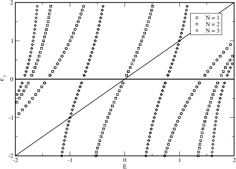
Figure 2: Curves satisfying the condition $T=1$ for $E$ and $\epsilon_{1}$ values as indicated. Only the cases $N=1,2,3$ are displayed.

Using the transfer matrix (23), we can apply equation (18) to get the transmission coefficient for this system. Since the presence of the generalized dimers in the chain introduce correlations in it, it is expected that particular values of the energy will produce transparent states. Unlike the RDM, where any site energy equal to the resonant energy produces a transparent states, we find that for this system, only certain values are allowed.

A relevant feature of this system is that, aside for this set of energies, there are also other values of $E$ for which the transmission is also equal to one. For any value of the impurity energy, one can always find one or more resonant energies. The number of resonant energies increases as the number of host sites between the impurities. This can be seen in Fig. (2), where we have plotted pairs of values of energy and site energy that produce a transparent state. Only the cases for 1 to 3 host sites are shown. Even though the figure shows a blank space between the points, the real data is continuous. For example, the relationship between $\epsilon_{1}$ and $E$ is

$$\epsilon_{1}=\frac{E^{2}-2}{E} \qquad N=1,$$ for (24)

$$\epsilon_{1}=\frac{E^{3}-3E}{E^{2}-1} \qquad N=2\,\,\mbox{and}$$ for (25)

$$\epsilon_{1}=\frac{E^{4}-4E^{2}+2}{E^{3}-2E} \qquad N=3.$$ for (26)

Similar expressions can be found for other values of $N$. The horizontal line is the case of zero site energy (regular lattice) for which we know that a continuous set of resonant energies exist. The diagonal line across the figure has been added to show those cases for which $E=\epsilon_{1}$ (see also table 1). From the crossing of this line with the curves we notice that the case of $N=3$ has two values of energy (-1 and 1). Apart from the trivial case $E=0$, the $N=1$ and $N=2$ cases have no extended states when $E=\epsilon_{1}$. Cases of $N\geq 3$ will always have resonant energies, but only for very particular values.

In Table 1, the resonant energies when $E=\epsilon_{1}$ are given for $N=1$ to $N=6$. Other values for $N>6$ can be easily found. The important point here is to notice the following two observations: 1) the number of resonant states is twice the number of the host sites in the generalized dimer ($2N$). 2) The resonant energy for $N$ host sites is also a resonant energy for any multiple of $N$. For example, for $N=3$, we have $E=1$, which is also a resonant energy for $N=6,9,12...$. Likewise, $E=\sqrt{2}$ is a resonant energy for $N=4,8,12...$, and so on.

Aside for this set of energies, there are also other values of $E\neq\epsilon_{1}$ for which the transmission is also equal to one. In fact, for any value of the impurity energy, one can always find one or more resonant energies. The number of resonant energies increases as the number of host sites between the impurities. It is not exactly equal to $N$ in all cases because it will depend on the crossing of the line of constant $\epsilon_{1}$ with the curves in Fig. (2). As we can see, there is a minimum value for which we will have $N+1$ states. This is shown in Fig. (3). Notice, also from Fig. 3 that, given the Fermi energy of the system, one can find a resonant energy close enough to it for a relatively small $N$.

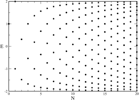
Figure 3: Resonant energies as a function of the number of host sites between the impurities. Here $\epsilon_{1}=1$.

In conclusion, we obtained the formula for the transmission coefficient in a compact and straightforward way, making use of the Cayley-Hamilton theorem and the transfer matrix method. We applied this formula in two cases: 1) for the $n$-dimer system and obtained previous results and 2) for a new system that we called a generalized dimer, consisting of two impurities embedded in the host lattice. This system was found to have resonant energies for $E=\epsilon_{1}$ and also for values of $E\neq\epsilon_{1}$. The number of these energies grows like the number of host sites between the impurities, $N$. This is an important feature of the system, since, by varying $N$, one can find a resonant energy close enough to the Fermi energy level. We believe that these kind of systems will be good candidates for the design of actual physical devices.

References

- (1) P. W. Anderson, Phys. Rev. 109, 1492 (1958).
- (2) J. C. Flores, Condens. Matter 1, 8471 (1989).
- (3) D. H. Dunlap, H-L. Wu and P. W. Phillips, Phys. Rev. Lett. 65, 88 (1990).
- (4) H-L Wu and P. Phillips, Phys. Rev. Lett. 66, 1366 (1991).
- (5) P. K. Datta, D. Giri and K. Kundu, Phys. Rev. B 47, 10727 (1993).
- (6) S. Sil, S. N. Karmakar and R. K. Moitra and A. Chakrabarti, Phys. Rev. B 48, 4192 (1993).
- (7) P. S. Davids, Phys. Rev. B 52, 4146 (1995).
- (8) F. M. Izrailev, T. Kottos, G. P. Tsironis, Phys. Rev. B 52, 3274 (1995).
- (9) E. Maciá and F. Domínguez-Adame, Phys. Rev. Lett. 76, 2957 (1996).
- (10) E. Lazo and M. E. Onell, Phys. Lett. A 283, 376 (2001).
- (11) G. Arfken, Mathematical Methods for Physicists, (Academic Press, New York, 1968).
- (12) S. Datta, Electronic Transport in Mesoscopic Systems, (Cambridge Univfersity Press, Cambridge, 1995).
- (13) R. A. Horn and C. R. Johnson, Matrix Analysis (Cambridge University Press, Cambridge, 1999).
- (14) Pedro Pereyra, Phys. Rev. Lett. 80, 2677 (1998).
- (15) A. Sánchez, F. Domínguez-Adame, G. Berman and F. Izrailev, Phys. Rev. B 51, 6769 (1995).
- (16) E. N. Economou, Green’s Functions in Quantum Physics (Springer-Verlag, Berlin, 1990).
- (17) M. P. Marder, Condensed Matter Physics (John Wiley and Sons, New York, 2000).