Spin Waves in Disordered III-V Diluted Magnetic Semiconductors

Abstract

We propose a new scheme for numerically computing collective-mode spectra for large-size systems, using a reformulation of the Random Phase Approximation. In this study, we apply this method to investigate the spectrum and nature of the spin-waves of a (III,Mn)V Diluted Magnetic Semiconductor. We use an impurity band picture to describe the interaction of the charge carriers with the local Mn spins. The spin-wave spectrum is shown to depend sensitively on the positional disorder of the Mn atoms inside the host semiconductor. Both localized and extended spin-wave modes are found. Unusual spin and charge transport is implied.

I Introduction

Diluted Magnetic Semiconductors (DMS) based on III-V semiconductors doped with Mn have attracted a lot of interest recently, after critical temperatures for the onset of ferromagnetism of the order of 110 K have been found in Ga_1-xMn_xAs, for $x=0.053$.Ohno ; Haya ; Esch More recently, critical temperatures larger than room temperatures have been reported in Mn-doped GaN, enhancing the hope for extensive technological applications of these materials.Hebard ; Sono

While there is general agreement that the magnetism is due to charge-carrier mediated, effectively ferromagnetic interactions between the Mn spins, there are various theoretical models attempting to understand their detailed behavior. The DMS are alloy systems, with inherent positional disorder of the Mn atoms; further, spin-orbit coupling may play a significant role for hole doping. A theoretical treatment which takes into account all these factors, and their effects on the magnetic and transport properties of DMS, is not yet available. Instead, theoretical models have tended to concentrate on different aspects of the problem.

One class of models, where much work has been done, neglects both the disorder and spin-orbit coupling effects. At large carrier densities, where Coulomb potentials of the impurity (Mn) atoms are effectively screened out, and other disorder effects (such as those coming from As antisite defects which are believed to be the cause of the large compensation observed experimentally) can be neglected, the former at least can be justified. In such a case, holes occupy a Fermi sea at the top of the valence band.RKKY Studies of the spin-wave spectraMacD , Monte-Carlo studiesMacDonald as well as dynamical mean-field theory studiesMillis have been performed. Overall, their results are rather similar to the physics one would expect to hold in a conventional ferromagnet. More recently, it has been proposed that spin-orbit coupling of the valence band, in the high carrier density (strongly metallic) regime leads to an RKKY coupling between Mn moments that is anisotropic in spin space, and where the positional disorder effectively leads to random anisotropy.Janko This would lead to frustration effects on the magnetic ordering, and therefore unusual ferromagnetism. A number of very useful ab-initio studies have also been published.Sanvito

In parallel, we have studied effects of positional disorder on the magnetic ordering (in the absence of spin-orbit coupling) of an impurity band model,MB1 ; MB2 ; Malcolm ; malcolm2 developed from previous work done in the context of insulating II-VI DMS compounds.Xin ; MB4 Such an approach should be of relevance at low doping concentrations x, at and below the metal-insulator transition, and possibly even above. Evidence for the existence of impurity-like states is provided by ab-initio studies,Sanvito which found that occupied hole states near the Fermi level have wave-functions mostly concentrated on and near the Mn impurity. More recently, Angle Resolved Photoemission Spectroscopy has revealed the existence of the impurity band in Ga_1-xMn_xAs with $x=0.035$ (very close to the metal-insulator transition).Okabayashi A scanning tunneling microscope study STM demonstrates the existence of an impurity band in (Ga,Mn)As samples with x=0.005-0.06. Optical spectroscopyBasov also identifies the impurity band for x=0.0001 and x=0.05 samples.

Electron densities in localized states, as well as states close to the mobility edge, can be far from homogeneous, unlike Bloch waves. At low Mn concentrations and high degree of compensation (which comes from charged centers) seen in DMS, short length-scale density fluctuations could be significant. This can lead to inhomogeneities in the local charge densities at different Mn sites, which in turn leads to (microscopically) inhomogeneous magnetizations of the magnetic ions in the ordered phase. Such inhomogeneity would be expected to alter the nature of the collective magnetic excitations (spin waves) of the magnetically ordered system, which in turn would affect charge transport through the magnetic excitation processes which give rise to spin-flip scattering.

In this paper, we develop a numerical scheme to calculate the spin wave spectrum for a finite but large size model of coupled fermions and spins, in the presence of quenched disorder. We show that the method accurately reproduces the results for a lattice model of small size obtained from a standard treatment of spin waves via the Random Phase Approximation.Negele ; Rowe ; Ripka We then apply the method to the model of Ref. MB1, , and study in detail its collective magnetic excitations.

The plan of the paper is as follows. The model Hamiltonian for DMS is described in section II. Section III is devoted to developing the numerical scheme. The accuracy of the scheme is tested by comparing it with the standard RPA method in section IV. In particular, we demonstrate that we can use our scheme to study large size systems, beyond the capability of the standard RPA approach. Section V presents the results obtained by applying the scheme to the model of Section II, including the density of states and nature of the eigenvectors of the magnetic excitations of the coupled fermion-spin system. We summarize our conclusions in section VI.

II The model

In the following we develop the formalism for an impurity band Hamiltonian that we believe to be appropriate for describing (at least qualitatively) the diluted magnetic semiconductor Ga_1-xMn_xAs for low doping $x$ (in the insulating phase, or not too far from the metal-insulator transition). However, generalizations of this method for other types of Hamiltonians, crystal structures, parameters etc. can be done in a straightforward manner.

The III-V host semiconductor is assumed to have the zinc-blende structure appropriate for GaAs. Experimental measurementsOhnorev suggest that valence-II Mn substitutes for valence-III Ga. As a result, the $N_{d}$ Mn dopants are randomly distributed at positions $\vec{R}_{i}$, $i=1,...,N_{d}$ on the $N\times N\times N$ FCC Ga sublattice, corresponding to $x=N_{d}/4N^{3}$. All throughout this paper, we assume periodic boundary conditions.

Due to the valence mismatch, each Mn introduces a charge carrier (hole) in the system. However, experimentally it is found that the hole concentration is considerably suppressed through compensation processes. As a result, the number of holes is only a fraction $p=10-30\%$ of the number of Mn atoms $N_{h}=pN_{d}$. Each Mn atom also has a ${5\over 2}-$spin $\vec{S}_{i}$ from its half-filled $3d$ level. The magnetic properties of the doped semiconductor are related to the exchange interaction between the Mn spins and the charge carrier spins. This interaction is known to be antiferromagnetic (AFM), and proportional to the probability of finding the charge carrier at the corresponding Mn site.

Recently, we proposed a simple impurity-band model to describe the behavior of the charge carriers for the low-doping regime.MB1 ; MB2 The main justification is that near and below the metal-insulator transition ($x\approx 0.03$) the density of charge carriers is not large enough to effectively screen the attractive Coulomb potential of the Mn dopants. As a result, bound, hydrogen-like impurity states are created about each Mn site, at an energy $E_{b}=1$ Ry above the top of the valence band. Due to interactions, these impurity states lead to the appearance of an impurity band, and the holes first occupy states in this band. Only if the concentration of holes (or the temperature) is large enough, are states in the valence band itself occupied by holes. Thus, it is reasonable to attempt a description of the charge carriers behavior only in terms of this impurity band.

As in previous work,MB1 ; MB2 in the following we will use the electron formalism to treat the problem. This is equivalent to performing a particle-hole transformation which leads to an inversion $E\rightarrow-E$ of the charge carrier spectrum. Thus, instead of emptying the top of a valence-like impurity band (i.e., introducing holes in the system) we instead occupy the bottom of a conduction-like impurity band. We also make the simplifying assumption that the isolated impurity wave-function for a charge carrier trapped near the Mn at site $\vec{R}_{i}$ is the $1s$ hydrogen orbital $\phi(\vec{r}-\vec{R}_{i})=\phi_{i}(\vec{r})\sim\exp{(-|\vec{r}-\vec{R}_{i}|/a_{B})}$, where $a_{B}=\hbar/\sqrt{2m^{*}E_{b}}=8$ Å is the appropriate Bohr radius related to the effective mass of the heavy hole ($m^{*}\approx 0.5m_{e}$ for GaAs) and the binding energy ($E_{b}=112.4$ meV for Mn in GaAs).BG Our approach neglects both the complicated orbital form of the acceptor wave-function (Ref. BG, ) and spin-orbit coupling. The former is not expected to lead to any qualitative changes. It has recently been proposed that spin-orbit coupling leads to frustration in the magnetic ordering.Janko These effects are left out in the present study, which concentrates on the effect of disorder. A study combining both effects is indicated for future work.

We consider the Hamiltonian

$${\cal H}=\sum_{i,j,\sigma}t_{ij}c^{\dagger}_{i\sigma}c_{j\sigma}+\sum_{i,j}J_{ij}\vec{S}_{i}\cdot\vec{s}_{j}.$$ (1)

Here, $c^{\dagger}_{i\sigma}$ creates a charge carrier with spin $\sigma$ in the impurity state centered at site $\vec{R}_{i}$. The first term describes the hopping of charge carriers between impurity states. We use the parameterization $t_{ij}=2(1+r/a_{\rm B})\exp{(-r/a_{\rm B})}$ Ry, where $r=|{\bf R}_{i}-{\bf R}_{j}|$, of magnitude and form appropriate for hopping between two isolated 1$s$ impurities which are not too close to one another. Bhatt1 This hopping term has been shown to lead to the appearance of an impurity band which has a mobility edge, as well as a characteristic energy for the occupied states in agreement with physical expectation.MB3

The second term of the Hamiltonian (1) describes the AFM exchange between the Mn spin ${\vec{S}}_{i}$ and the charge carrier spin ${\vec{s}}_{j}={1\over 2}c^{\dagger}_{j\alpha}{\vec{\sigma}}_{\alpha\beta}c_{j\beta}$ [${\vec{\sigma}}$ are the Pauli spin matrices]. This AFM exchange is proportional to the probability of finding the charge carrier trapped at ${\vec{R}}_{j}$ near the Mn spin at ${\vec{R}}_{i}$, and therefore $J_{ij}=J|\phi_{j}(\vec{R}_{i})|^{2}=J\exp{\left(-2|{\vec{R}}_{i}-{\vec{R}}_{j}|/a_{B}\right)}$. Based on calculations of the isolated Mn impurity in GaAs, we estimate the exchange coupling between a hole and the trapping Mn ($\vec{R}_{i}=\vec{R}_{j}$) to be $J=15$ meV.MB1 ; BG As already stated, the number of Mn atoms is $N_{d}$, and therefore there are a total of $2N_{d}$ states in the impurity band. The number of charge carriers is fixed to $N_{h}=pN_{d}$, where we take $p=10\%$.

In Ref. MB2, we studied the relevance of various other terms, such as an on-site potential (associated with the Coulomb potential of the compensation centers), Hubbard-like on-site repulsion (describing interactions between charge-carriers), external magnetic field etc. While they lead to various quantitative changes, we believe that the qualitative picture we present in the following sections is not changed by their absence.

III The collective mode spectrum

The Random Phase Approximation (RPA) describes the collective excitations of a system about its self-consistent $T=0$ mean-field ground state. In order to clarify the notation used, we begin this section with a very short review of the derivation of the relevant equations for the mean-field ground state.

III.1 The mean-field ground state

We use the equation-of-motion approach of Ref. Rowe, . At the mean-field level, we are trying to find non-interacting fermionic quasiparticles through a unitary transformation of the on-site charge carrier operators:

$$a^{\dagger}_{n\sigma}=\sum_{i}\psi_{n\sigma}(i)c^{\dagger}_{i\sigma}$$ (2)

such that

$$[{\cal H},a^{\dagger}_{n\sigma}]\approx E_{n\sigma}a^{\dagger}_{n\sigma}$$ (3)

and

$$[{\cal H},S_{i}^{+}]\approx-\hbar H_{i}S_{i}^{+}$$ (4)

For a non-interacting system, Eqs. (3) and (4) would be exact. For an interacting system at the mean-field level, the exact Hamiltonian is approximated by the diagonalized, non-interacting Hartree-Fock Hamiltonian

$${\cal H}\rightarrow{\cal H}_{HF}=\sum_{n\sigma}E_{n\sigma}a^{\dagger}_{n\sigma}a_{n\sigma}-\sum_{i}H_{i}S^{z}_{i}$$ (5)

for which Eqs. (3) and (4) become exact.

It is straightforward to show that for Hamiltonian (1)

$$[{\cal H},a^{\dagger}_{n\sigma}]=\sum_{ij}t_{ij}\psi_{n\sigma}(j)c^{\dagger}_{i\sigma}+\sum_{ij}J_{ij}\vec{S}_{j}{\vec{\sigma}_{\alpha\sigma}\over 2}\psi_{n\sigma}(i)c^{\dagger}_{i\alpha}$$ (6)

The right-hand-side of Eq. (6) contains spin operators, so it cannot be put in the form of Eq. (3) unless we linearize it, by replacing the spin operators with their mean-field ground state expectation value $\vec{S}_{j}\rightarrow\langle\vec{S}_{j}\rangle=\hat{e}_{z}S_{Mn}(j)$. While the choice of a collinear ground-state, with all Mn spins aligned along the $z$-axis, is not the most general possibility, we have actually shown in Ref. MB2, that the ground-state of this model, for the range of parameters we are interested in, is indeed collinear. This is why we choose to apriori make this assumption in this case.

After the linearization, we can now equate the right-hand-side of Eq. (6) with $E_{n\sigma}a^{\dagger}_{n\sigma}$ [see Eq. (3)] to obtain the Hartree-Fock equation for the one-particle orbitals:

$$E_{n\sigma}\psi_{n\sigma}(i)=\sum_{j}t_{ij}\psi_{n\sigma}(j)+\sum_{j}J_{ij}S_{Mn}(j){\sigma\over 2}\psi_{n\sigma}(i)$$ (7)

The mean-field ground-state of the charge carriers is obtained by occupying the $N_{h}$ lowest-energy orbitals,

$$|\Psi\rangle_{cc}=\prod_{(n\sigma)=1}^{N_{h}}a^{\dagger}_{n\sigma}|0\rangle$$ (8)

The effective magnetic fields $H_{i}$ [see Eq. 5)] are obtained in a similar way. We evaluate the commutator of the exact Hamiltonian with the spin raising operator $S_{i}^{+}=S_{i}^{x}+iS_{i}^{y}$

$$[{\cal H},S_{i}^{+}]=-\hbar\sum_{j}J_{ij}S_{i}^{z}s_{i}^{+}+\hbar\sum_{j}J_{ij}S_{i}^{+}s_{i}^{z}$$ (9)

The right-hand-side now contains charge carrier operators (in the charge carrier spin operator), beside the spin operators. We again use linearization $s_{i}^{+}\rightarrow\langle s_{i}^{+}\rangle=0$ [see Eq. (8)], $s_{i}^{z}\rightarrow\langle s_{i}^{z}\rangle=s_{h}(i)$, and by comparison with Eq. (4) we find

$$H_{i}=-\sum_{j}J_{ij}s_{h}(j)$$ (10)

From Eq. (5) we see that if $H_{i}>0$, then in the mean-field ground state the spin $\vec{S}_{i}$ is in the “up” state $|+S\rangle$ and therefore $S_{Mn}(i)=+S$, while if $H_{i}<0$ the spin $\vec{S}_{i}$ is in the “down” state $|-S\rangle$ and $S_{Mn}(i)=-S$ ($S=5/2$). As a result, the spin-part of the mean-field ground-state can also be easily found if the expectation value of the charge carrier spins $s_{h}(j)$ are known from Eqs. (7), (8). Thus, we obtain the usual self-consistent Hartree-Fock equations.

Diluted Magnetic Semiconductors exhibit ferromagnetism at low temperatures. As a result, we assume that in the mean-field ground state, all Mn spins are fully polarized $S_{Mn}(i)=+S$. Then, from Eq. (7) we find the lowest-lying $N_{h}$ states. If the charge carriers are also fully polarized at $T=0$, all the occupied $N_{h}$ state have $\sigma=\downarrow$, and therefore the mean-field ground-state is of the form:

$$|\Psi\rangle=\prod_{n=1}^{N_{h}}a^{\dagger}_{n\downarrow}|0\rangle\otimes|S,S,....,S\rangle$$ (11)

Of course, one must check that self-consistency is obeyed by verifying that indeed the first $N_{h}$ lowest energy one-electron states are all spin-down. We find that this always holds true for the parameters we study in this paper. As discussed later, the spin-wave spectrum of the collective excitations also confirms that this ground-state is indeed stable. However, for higher charge carrier concentrations (or Hamiltonians with other types of interactions) it is likely that the HF ground-state is only partially spin polarized. In that case, one must do the full iterational search for the self-consistent HF ground state. The computation for the spin-wave spectrum in the partially-polarized case (for instance due to spin-orbit coupling), can be derived in a similar way to the one we present in the following for the fully polarized case.

III.2 The Random Phase Approximation

We will use the same equation-of-motion approach to derive the RPA equations. We are interested in spin-waves, which are related to spin-flip (spin-lowering) processes. Therefore, the RPA operators for spin-wave collective modes must be constructed in terms of spin-flip operators

$$\left\{\begin{array}[c]{c}b^{\dagger}_{hp}=a^{\dagger}_{h\uparrow}a_{p\downarrow}\\ B^{\dagger}_{i}={1\over\sqrt{2S}}S^{-}_{i}\\ \end{array}\right.$$ (12)

The index $h=1,N_{d}$ runs over the empty (“hole”) states of the HF ground state, while the index $p=1,N_{h}$ runs over the occupied (“particle”) states of the HF ground state. The index $i=1,N_{d}$ runs over all the Mn spin positions. The HF ground-state $|\Psi\rangle$ is fully polarized, and given by Eq. (11).

The spin-flip operators have “bosonic” nature, as expected for collective modes operators. Indeed, it is straightforward to verify that $\langle\left[b_{hp},b^{\dagger}_{h^{\prime}p^{\prime}}\right]\rangle=\delta_{pp^{\prime}}\delta_{hh^{\prime}}$, $\langle\left[B_{i},B^{\dagger}_{j}\right]\rangle=\delta_{ij}$, with all the other commutators identically zero. Here, the notation $\langle...\rangle$ signifies an average over the HF ground state $\langle\Psi|...|\Psi\rangle$.

The Hamiltonian can be rewritten in terms of the $a_{n\sigma}$ operators as [see Eqs. (1), (2)]

$${\cal H}=\sum_{n,m,\sigma}t_{nm\sigma}a^{\dagger}_{n\sigma}a_{m\sigma}+\sum_{n,m,i\atop\alpha\beta}J_{n\alpha,m\beta}(i)a^{\dagger}_{n\alpha}a_{m\beta}\vec{\sigma}_{\alpha\beta}\cdot\vec{S}_{i}$$ (13)

where

$$t_{nm\sigma}=\sum_{i,j}t_{ij}\psi^{*}_{n\sigma}(i)\psi_{m\sigma}(j)$$

and

$$J_{n\alpha,m\beta}(i)={1\over 2}\sum_{j}J_{ij}\psi_{n\alpha}^{*}(j)\psi_{m\beta}(j).$$ (14)

One can easily derive the equations of motion for the spin-flip operators. For instance

$$[{\cal H},B^{\dagger}_{i}]={2\over\sqrt{2S}}\sum_{nm}J_{n\downarrow,m\uparrow}(i)a^{\dagger}_{n\downarrow}a_{m\uparrow}S^{z}_{i}$$

$$-{1\over\sqrt{2S}}\sum_{nm\sigma}J_{n\sigma,m\sigma}(i)\sigma a_{n\sigma}^{\dagger}a_{m\sigma}S^{-}_{i}$$ (15)

Since RPA is an approximation, not an exact solution, we again must linearize this commutator about the HF ground-state, and keep only the meaningful terms. In other words, we replace

$$a^{\dagger}_{n\downarrow}a_{m\uparrow}S^{z}_{i}\rightarrow\langle a^{\dagger}_{n\downarrow}a_{m\uparrow}\rangle S^{z}_{i}+a^{\dagger}_{n\downarrow}a_{m\uparrow}\langle S^{z}_{i}\rangle\rightarrow Sa^{\dagger}_{n\downarrow}a_{m\uparrow}$$

Here, the first transformation is the linearization about the HF ground state $|\Psi\rangle$. The second transformation results if one uses the HF expectation values $\langle S^{z}_{i}\rangle=S$, $\langle a^{\dagger}_{n\downarrow}a_{m\uparrow}\rangle=0$. The restriction to relevant terms means that in any sum over $(n\downarrow)$, we restrict $n$ to being an occupied orbital in the HF ground-state $1\leq n\leq N_{h}$, because otherwise $b_{mn}^{\dagger}|\Psi\rangle=0$, i.e. a spin-flip process from the HF ground-state is impossible [see Eq. (12)]. Performing a similar linearization for $a_{n\sigma}^{\dagger}a_{m\sigma}S^{-}_{i}$ and collecting the various terms, we find the linearized equation of motion

$$[{\cal H},B^{\dagger}_{i}]\approx H_{i}B_{i}^{\dagger}+\sqrt{2S}\sum_{p=1}^{N_{h}}\sum_{h=1}^{N_{d}}J_{p\downarrow,h\uparrow}(i)b_{hp}$$ (16)

After similar steps, the linearized equation of motion for the other spin-flip operator $b_{hp}$ is found to be

$$[{\cal H},b_{hp}]\approx-\left(E_{h\uparrow}-E_{p\downarrow}\right)b_{hp}-\sqrt{2S}\sum_{i}J^{*}_{p\downarrow,h\uparrow}(i)B_{i}^{\dagger}$$ (17)

Eqs. (16) and (17) allow us to “guess” the RPA part of the Hamiltonian, for which Eqs. (16) and (17) become exact, to be given by

$${\cal H}_{RPA}=\sum_{h=1}^{N_{d}}\sum_{p=1}^{N_{h}}\left(E_{h\uparrow}-E_{p\downarrow}\right)b^{\dagger}_{hp}b_{hp}+\sum_{i}H_{i}B^{\dagger}_{i}B_{i}$$

$$+\sqrt{2S}\sum_{i}\sum_{h=1}^{N_{d}}\sum_{p=1}^{N_{h}}\left(J_{p\downarrow,h\uparrow}(i)B_{i}b_{hp}+h.c.\right)$$ (18)

Thus, the RPA Hamiltonian is quartic in electron operators and quadratic in spin operators, showing that it is the next order term after the Hartree-Fock Hamiltonian (which is quadratic in electron operators and linear in spin operators)

$${\cal H}={\cal H}_{HF}+{\cal H}_{RPA}+....$$

Higher order approximation terms describe interactions between the collective modes, which are neglected at the RPA level.

We want to diagonalize the RPA Hamiltonian to the canonical form

$${\cal H}_{RPA}=\sum_{\alpha}\hbar\Omega_{\alpha}Q^{\dagger}_{\alpha}Q_{\alpha}$$ (19)

where $Q^{\dagger}_{\alpha}$ is the creation operator for a spin-wave with energy $\hbar\Omega_{\alpha}$, and $\alpha$ is an index (in homogeneous systems, it would be a wave-vector). Since they create collective mode excitations, these operators must have bosonic nature $[Q_{\alpha},Q_{\beta}]=0$. However, since they do not describe exact, but only approximative solutions of the exact Hamiltonian, in fact only the weaker condition $\langle[Q_{\alpha},Q^{\dagger}_{\beta}]\rangle=\delta_{\alpha\beta}$ is obeyed. The most general form for these operators [see Eq. (18)] is

$$Q^{\dagger}_{\alpha}=\sum_{h=1}^{N_{d}}\sum_{p=1}^{N_{h}}X_{hp}^{(\alpha)}b_{hp}+\sum_{i}Y_{i}^{(\alpha)}B^{\dagger}_{i}$$ (20)

Using the equation of motion $[{\cal H}_{RPA},Q^{\dagger}_{\alpha}]=\hbar\Omega_{\alpha}Q^{\dagger}_{\alpha}$ and computing the commutator using Eqs. (18), (20), we find the diagonalization condition to be

$$\left[\hbar\Omega_{\alpha}+E_{h\uparrow}-E_{p\downarrow}\right]X^{(\alpha)}_{hp}=\sqrt{2S}\sum_{i}J_{p\downarrow,h\uparrow}(i)Y^{(\alpha)}_{i}$$ (21)

$$\left[\hbar\Omega_{\alpha}-H_{i}\right]Y^{(\alpha)}_{i}=-\sqrt{2S}\sum_{p=1}^{N_{h}}\sum_{h=1}^{N_{d}}J_{p\downarrow,h\uparrow}^{*}(i)X^{(\alpha)}_{hp}$$ (22)

These are the RPA equations and they can be recast in the customary standard eigenvalue RPA equation formRipka

$$\hbar\Omega\left(\begin{array}[c]{c}{\bf X}\\ {-\bf Y}\\ \end{array}\right)=\left(\begin{array}[c]{cc}{\bf E}&{\bf J}\\ {\bf J}^{*}&{\bf H}\\ \end{array}\right)\cdot\left(\begin{array}[c]{c}{\bf X}\\ {\bf Y}\\ \end{array}\right)$$ (23)

where the vectors ${\bf X}$ and ${\bf Y}$ contain all the unknowns $X_{hp}$ and $Y_{i}$, and the matrices ${\bf E},{\bf H}$ and ${\bf J}$ have the elements ${\bf E}_{hp,h^{\prime}p^{\prime}}=-\delta_{hh^{\prime}}\delta_{pp^{\prime}}(E_{h\uparrow}-E_{p\downarrow})$, ${\bf H}_{i,i^{\prime}}=-\delta_{i,i^{\prime}}H_{i}$ and ${\bf J}_{hp,i}=\sqrt{2S}J_{p\downarrow,h\uparrow}(i)$.

The dimension of the RPA matrix (23), and therefore the number of normal modes, is $N_{d}+N_{h}\times N_{d}$. Of these solutions, $N_{d}$ are proper spin-wave collective modes, while the rest of $N_{h}\times N_{d}$ are spin-flip processes associated with particle-hole excitations. If there were no interactions (J=0), the eigenenergies of these spin-flip processes would be $H_{i}$ for the lowering of the Mn spin $i$, respectively $E_{h\uparrow}-E_{p\downarrow}$ for a hole spin-flip [see the left-hand side of Eqs. (21),(22)]. Interactions renormalize these values [as described by the right-hand-side of Eqs. (21),(22)], but one still expects $N_{d}$ spin-wave collective solutions at low energies, coming from the Mn spin lowering, and $N_{h}\times N_{d}$ spin-flip particle-hole excitations at energies comparable or larger than the spin-flip gap $\Delta=E_{1\uparrow}-E_{N_{h}\downarrow}$.

We now comment on the sign of the RPA spectrum frequencies $\hbar\Omega_{\alpha}$. Since $H_{i}>0$ [see Eq. (10)] and $E_{h\uparrow}-E_{p\downarrow}>0$ (by definition of the HF ground-state), it is apparent from Eqs. (21),(22) that $N_{d}$ spin-wave solutions will have positive energies $\hbar\Omega_{\alpha}$, while the $N_{h}\times N_{d}$ spin-flip particle-hole excitations will have negative energies. This does not imply that the system is unstable, but simply that we have not chosen the proper spin-flip creation operators. Instead of the choice of Eq. (20), we can also denote

$$P_{\alpha}=Q^{\dagger}_{\alpha}=\sum_{h=1}^{N_{d}}\sum_{p=1}^{N_{h}}X_{hp}^{(\alpha)}b_{hp}+\sum_{i}Y_{i}^{(\alpha)}B^{\dagger}_{i}$$ (24)

In terms of these new operators, we have now $[{\cal H}_{RPA},P_{\alpha}]=\hbar\Omega_{\alpha}P_{\alpha}$, i.e.

$${\cal H}_{RPA}=\sum_{\alpha}(-\hbar\Omega_{\alpha})P^{\dagger}_{\alpha}P_{\alpha}$$ (25)

In other words, a negative solution for $\hbar\Omega$ simply means that we chose the corresponding annihilation operator instead of the creation operator when we wrote Eq. (20). For spin-flip processes, it is obvious that this is the case from the dependence of $Q^{\dagger}_{\alpha}$ on $b_{hp}$, instead of $b_{hp}^{\dagger}$.

An unstable mean-field ground-state is signaled by complex values of the spectrum frequencies $\hbar\Omega_{\alpha}$.Rowe ; Ripka Excited states about the mean-field ground-state $|\Psi\rangle$ are of the general form $|\Phi\rangle=[1+\sum c_{\alpha}(Q^{\dagger}_{\alpha})^{n_{\alpha}}]|\Psi\rangle$. Within RPA the dynamics of such states is dictated by ${\cal H}_{RPA}$, leading to a time dependence:

$$|\Phi(t)\rangle=e^{-iE_{HF}t/\hbar}[1+\sum_{\alpha}c_{\alpha}e^{-in_{\alpha}\Omega_{\alpha}t}(Q^{\dagger}_{\alpha})^{n_{\alpha}}]|\Psi\rangle,$$

where $E_{HF}=\langle\Psi|{\cal H}|\Psi\rangle$ is the Hartree-Fock energy of the system. If any of the frequencies $\Omega_{\alpha}$ has a non-trivial imaginary part, it follows that the expectation value of any operator $\langle\Phi(t)|...|\Phi(t)\rangle$ will move in time exponentially away from its mean-field ground-state expectation value $\langle\Psi|...|\Psi\rangle$, i.e. the mean-field is unstable to small perturbations.

The advantage of the standard RPA approach is that by solving the eigenvalue problem (23), one finds the normal mode spectrum $\hbar\Omega$ and the spatial distribution of the spin-waves (related to the $Y_{i}$ coefficients) at once. The obvious disadvantage is of a numerical nature: for a disordered system the RPA matrix must be diagonalized numerically. The size of the matrix is $n=(1+N_{h})N_{d}$. The typical sizes we consider are systems with around $N_{d}=500$ Mn spins, and $N_{h}=50=10\%N_{d}$ holes (although concentrations up to $30\%$ might have to be considered, depending on the doping $x$), leading to RPA matrices of typical size $n>25,000$. As a result, one has to either consider much smaller systems (in which case, finite size effects may be overwhelmingly important), or to try sparse matrix techniques to obtain the first few low-energy modes of the RPA matrix (although the off-diagonal ${\bf J}$ matrix is not necessarily sparse).

There is, however, an alternative way of finding the collective mode spectrum and spatial distributions. We can directly solve for the $X_{hp}$ coefficients from Eq. (21) and rewrite Eq. (22) as

$$\sum_{i^{\prime}}M_{ij}(\omega)Y_{j}(\omega)=\hbar\omega Y_{i}(\omega)$$ (26)

where

$$M_{ij}(\omega)=\delta_{ij}H_{i}-2S\sum_{p=1}^{N_{h}}\sum_{h=1}^{N_{d}}{J^{*}_{p\downarrow,h\uparrow}(i)J_{p\downarrow,h\uparrow}(j)\over\hbar\omega+E_{h\uparrow}-E_{p\downarrow}+i\eta}$$ (27)

The advantage of this formulation is that one has to deal with much smaller matrices (the dimension of the ${\bf M}$ matrix is $N_{d}=500$). Eq. (26) tells us that for frequencies $\Omega$ belonging to the spin-wave spectrum, the matrix ${\bf M}(\Omega)$ has at least one eigenvector corresponding to an eigenvalue $\lambda(\Omega_{\alpha})=\hbar\Omega_{\alpha}$ (if the mode is degenerate, there are several such eigenvectors). The corresponding eigenvectors give us the desired spatial mode distribution $Y_{i}^{(\alpha)}=Y_{i}(\Omega_{\alpha})$. Thus, the problem is reduced to sweeping the range of frequencies of interest (for low-energy collective excitations, this is usually a fairly small range of frequencies near $\omega=0$), and monitoring the eigenvalues of the ${\bf M}(\omega)$ matrix. The dependence on $\omega$ of the matrix elements $M_{ii^{\prime}}(\omega)$, and therefore of the eigenvalues $\lambda(\omega)$ is monotonic for small $\omega\ll\Delta$ [see Eq. (27)]. As a result, each equation $\lambda(\omega)=\hbar\omega$ has a single solution, and we expect to find $N_{d}$ collective mode eigenenergies, one for each eigenvalue. The monotonic dependence of $\lambda(\omega)$ on $\omega$ also simplifies the search for the collective spectrum, since it is enough to evaluate the eigenvalues $\lambda(\omega)$ in the range of interest on a grid of step $\delta\omega$, and use linear interpolation to find the solutions of the equations $\lambda(\omega)=\hbar\omega$. As we show in the following by comparison with standard RPA (for small system sizes) we can very easily achieve relative errors less than $10^{-5}$.

The RPA spectrum has a second type of solutions, the spin-flip particle-hole continuum. These solutions are at frequencies of the order of the gap between the last occupied and first empty HF states $\hbar\omega\sim\Delta$, and one expects $N_{h}\times N_{d}$ such solutions. In principle, one can use the same method to find these energies as well, although the fact that they extend over a larger range of frequencies and that the $\omega$ dependence is very strong makes the search more difficult. Typically, one is only interested in the lower and upper limits of the spin-flip continuum, which can be found easily with the method just described.

Finally, we would like to mention that it is always possible to reformulate the standard RPA equation (23) in a “self-consistent” form of the type shown in Eq. (26), with a matrix ${\bf M}(\omega)$ of much smaller dimension than the RPA matrix. For instance, for Hamiltonians describing interacting electron systems, the RPA matrix has a dimension $\sim N_{o}N_{e}$, where $N_{o}$ is the number of occupied, and $N_{e}$ is the number of empty orbitals in the mean-field ground-state.Ripka For a system with a finite concentration of electrons $x$ on a lattice of linear dimension $N$ in a $D$-dimensional space, we have $N_{o}\sim xN^{D}$ and $N_{e}\sim(1-x)N^{D}$, and the RPA matrix scales as $x(1-x)N^{2D}$. For such systems, one can always find an equivalent reformulation of the RPA equation in terms of a ${\bf M}(\omega)$ matrix of size $\sim N^{D}$.thesis This allows numerical handling of considerably larger systems, without having to resort to sparse matrix techniques, which often have issues related to instability.

IV Implementation

In this section we show, by direct comparison against known calculations, as well as by direct comparison against solving the RPA matrix equation, that the formulation of Eqs. (26), (27) gives correct and numerically very accurate results. In the second part of the section we describe in more detail the numerical implementation as well as efficiency of our method.

IV.1 Analytical solution

We first apply our approach by solving Eqs. (26), (27) analytically for a simplified case. We assume that the Mn spins are arranged on an ordered superlattice, instead of having random positions. Then, the charge-carrier part of the mean-field Hamiltonian is easily diagonalized in the $\vec{k}$-space:

$${\cal H}_{cc}^{HF}=\sum_{\vec{k}\sigma}E_{\vec{k}\sigma}c^{\dagger}_{\vec{k}\sigma}c_{\vec{k}\sigma}$$ (28)

where

$$E_{\vec{k}\sigma}=\epsilon_{\vec{k}}+{J_{0}S\over 2}\sigma$$ (29)

Here, $\epsilon_{\vec{k}}=\sum_{\vec{\delta}\neq 0}t_{\vec{\delta}}\exp{(i\vec{k}\cdot\vec{\delta})}$ is the kinetic energy of the non-interacting electrons, where $\vec{\delta}$ indexes all the neighboring sites and $t_{\vec{\delta}}=t_{ij}$ for which $|\vec{R}_{i}-\vec{R}_{j}|=|\vec{\delta}|$. Also, $J_{0}=\sum_{\vec{\delta}}J_{\vec{\delta}}$, where again $J_{\vec{\delta}}=J_{ij}$ for which $|\vec{R}_{i}-\vec{R}_{j}|=|\vec{\delta}|$. In the HF ground state, the states $(\vec{k},\downarrow)$ given by the condition $N_{h}=\sum_{|\vec{k}|<k_{F}}1$ are occupied. Since the $N_{h}$ electrons are equally distributed among the $N_{d}$ Mn sites, and are fully polarized, the z-component of the total spin created by electrons at each site, within HFA, is $s_{h}(j)=-{1\over 2}{N_{h}\over N_{d}}=-{p/2}$, and therefore we find $H_{i}=J_{0}p/2$ [see Eq. (10)].

Using the fact that the solutions of Eq. (26) must also have plane-wave structure $Y_{i}\sim\exp{(i\vec{Q}\cdot\vec{R}_{i})}$, it follows that the index $\alpha\rightarrow\vec{Q}$ becomes a wave-vector, as expected, and we can reduce Eqs. (26) and (27) to a self-consistent equation for each collective mode $\hbar\omega(\vec{Q})$:

$$\hbar\omega-{pJ_{0}\over 2}=-{S|J(\vec{Q})|^{2}\over 2N_{d}}\sum_{\vec{k}}{f(E_{\vec{k},\downarrow})\over\hbar\omega+\epsilon_{\vec{k}-\vec{Q}}-\epsilon_{\vec{k}}+J_{0}S}$$ (30)

Here, $J(\vec{Q})=\sum_{\vec{\delta}}\exp{(i\vec{Q}\cdot\vec{\delta})}J_{\vec{\delta}}$. The occupation number $f(E_{\vec{k},\downarrow})$ obviously comes from the sum over occupied states we had in Eq. (27). For a finite-size ordered lattice, one expects considerable degeneracy for each mode $E_{\vec{k}\sigma}$, due to invariance to various symmetry transformations of the $\vec{k}$-vector. In most cases, the number of charge carriers is such that the last orbital (of degeneracy $G$) is only partially occupied by $g$ charge carriers. In this case, one must obviously choose $f=g/G$ for all these orbitals, and $f=1$ for lower, fully occupied orbitals, and $f=0$ for higher, empty orbitals. Otherwise, the translational invariance is broken and the collective spectrum is not indexed by a wave-vector.

The sum in Eq. (30) can be performed if we assume that the dispersion at the bottom of the band is of quadratic form $\epsilon_{\vec{k}}=\hbar^{2}k^{2}/(2m)$ (this is a reasonable approximation since we are interested in low filling fraction $p$). Then, the sum over occupied states can be transformed to an integral which is straightforward to evaluate, leading to the solution:

$$\hbar\omega={pJ_{0}\over 2}+|J(\vec{Q})|^{2}{3pS\over 4v_{F}}{1\over Q}f(\omega,{Q})$$ (31)

Here, $v_{F}=\hbar k_{F}/m$ is the Fermi velocity, where the Fermi vector is given by

$$N_{h}=pN_{d}={V\over(2\pi)^{3}}{4\pi k_{F}^{3}\over 3}.$$

The function $f(\omega,Q)$ is given by

$$f(\omega,Q)=-{{\hbar\omega+\epsilon_{Q}+J_{0}S}\over v_{F}Q}$$

$$+{1\over 2}\left[1-\left({{\hbar\omega+\epsilon_{Q}+J_{0}S}\over v_{F}Q}\right)^{2}\right]\ln{{\hbar\omega+\epsilon_{Q}+J_{0}S-v_{F}Q}\over{\hbar\omega+\epsilon_{Q}+J_{0}S+v_{F}Q}}$$

where $\epsilon_{Q}=\hbar^{2}Q^{2}/2m$.

For comparison purposes, we will assume a local AFM interaction $J_{ij}\rightarrow cJ_{pd}\delta_{ij}$, leading to $J(\vec{Q})=J_{0}=cJ_{pd}$. In this case, the Hamiltonian becomes identical to the Hamiltonian used by Konig. et. al in Ref. MacD, , provided that the effective mass $m$ in the dispersion relation is assumed to be the band effective mass. We can easily solve Eq. (31) in the asymptotic limit $Q\rightarrow 0$, to find

$$\hbar\omega(\vec{Q})={\hbar^{2}Q^{2}\over 2m}{1\over 2S/p-1}\left[1-{4\over 5}{t\over J_{0}S}\left({p\over 6\pi^{2}}\right)^{2/3}\right]$$ (32)

This is indeed identical with the asymptotic long-wavelength spin-wave spectrum obtained in Ref. MacD, , and has the typical quadratic dependence of spin-waves in conventional ferromagnetic systems.

IV.2 Direct comparison between the two formulations

In this section we briefly illustrate the accuracy and speed of our formulation of the RPA problem [Eqs. (26) and (27)], in comparison with the standard RPA approach [Eq. (23)]. We use a rather small system, with $N_{d}=80$ Mn spins randomly distributed on a FCC lattice with linear size $N=10$, corresponding to a Mn concentration $x=N_{d}/4N^{3}=0.02$. The number of charge carriers is $N_{h}=pN_{d}=8$, and the other parameters are as defined in Section II. Thus, the standard RPA involves the diagonalization of a non-hermitian matrix of dimension $720$.

Figure 1: The largest eight eigenvalues $\lambda(\omega)$ of the ${\bf M}(\omega)$ matrix (circles), evaluated on a grid with a step $\delta\omega=0.05$ meV. The full line is $\hbar\omega$. The spin-wave spectrum is given by the condition $\lambda\omega=\hbar\omega$.

Figure 2: Accuracy $\Delta\omega/\omega_{RPA}$ for all $N_{d}=80$ spin-wave frequencies $\omega_{RPA}$, between the exact RPA (standard) values and values obtained in our formulation using a grid with $\delta\omega=0.05$ [see Fig. 1].

In Fig. 1 we show the $\omega$-dependence of the largest eight eigenvalues $\lambda(\omega)$ of the ${\bf M}$ matrix (circles), evaluated on a grid with a step $\delta\omega=0.05$ meV. [For real $\omega$ and $\eta=0$, the matrix ${\bf M}(\omega)$ is hermitian and all eigenvalues $\lambda(\omega)$ are real, see Eq. (27)]. The full line is $\hbar\omega$, and the spin-wave spectrum is given by the condition $\lambda(\omega)=\hbar\omega$. One can see that the eigenvalues $\lambda(\omega)$ have monotonically increasing dependence on $\omega$ for small $\omega\ll\Delta\approx 50$ meV, and therefore the equation $\lambda(\omega)=\hbar\omega$ can have at most one solution for each eigenvalue, for small $\omega$. If each eigenvalue yields a solution, we have found all $N_{d}$ spin-wave frequencies. If one or more eigenvalues do not intersect the $\hbar\omega$ line, this means that the mean-field ground-state is unstable ( there are complex spin-wave frequencies). For all the cases and parameters we investigate, we found that the fully-polarized ground-state is stable for our model.

Figure 3: Largest relative error $\Delta\omega/\omega_{RPA}$ among $5N_{d}=400$ spin-wave frequencies $\omega_{RPA}$, between the exact RPA (standard) values and values obtained in our formulation using a grid with $\delta\omega=0.05,0.1,0.2,0.3,0.4,0.5,0.75$ and 1 meV. The line is drawn to guide the eye. Even for a very large grid, the relative error is still reasonably small.

To find the spectrum frequencies $\hbar\Omega_{\alpha}$, we use linear interpolation over the interval $\delta\omega$ where each $\lambda(\omega)$ curve intersects the $\hbar\omega$ curve. This method avoids the need of evaluating the eigenvalues at too many $\omega$ points (the most time-consuming part of the computation is the evaluation of the matrix elements of ${\bf M}$). The high degree of accuracy obtained with this method is demonstrated in Fig. 2, where we compare the exact RPA spectrum $\omega_{RPA}$ obtained through direct diagonalization of the RPA matrix [see Eq. (23)] with the the values ${\tilde{\omega}}_{RPA}$ obtained through our formulation. In fact, we plot the relative error $\Delta\omega/\omega_{RPA}=({\tilde{\omega}}_{RPA}-\omega_{RPA})/\omega_{RPA}$ for each spectrum frequency $\omega_{RPA}$. As one can see from Fig. 2, the largest error is of the order $2\cdot 10^{-6}$, for the grid $\delta\omega=0.05$.

This suggests that one could use a much larger grid $\delta\omega$ and still have a good accuracy. Indeed, we have computed the spectrum through both methods for five different realization of disorder, using various grid values $\delta\omega$ in our formulation, and selected the largest relative error for each case (from a total of $5N_{d}=400$ values). The results are shown in Fig. 3. The error is found to scale as the square of the grid size. Even with a very large grid $\delta\omega=1$ meV, (which implies the evaluation of the eigenvalues $\lambda(\omega)$ in only very few points), we still get a relative error smaller than $10^{-3}$. Thus, one can use the grid step $\delta\omega$ to optimize and considerably speed up the computation. However, as the number of spins (and eigenvalues) $N_{d}$ increases, one must take into consideration other complications, as discussed below.

Figure 4: CPU time for the two RPA methods, for systems with $N_{d}=64,125$ and 216 spins. The standard RPA (full line) is significantly more time consuming than our formulation (dashed line).

In Fig. 4 we compare CPU times for finding the RPA spin-wave spectrum using the standard vs. our RPA formulations. All simulations were done on the same processor. We used a small grid $\delta\omega=0.05$ meV for our approach, and verified that all relative errors were less than $10^{-5}$. We use systems with $N_{d}=64,125$ and 216 spins, randomly distributed on FCC lattices of linear size $N=12,15$ and 18 ($x=0.0092,p=10\%$). As expected, the computational time depends in a power-law manner on the size $N_{d}$, with exponents 6.4 and 3.2 respectively for the standard and current approach. Clearly, our formulation can be successfully used for much larger sizes than those afforded by the standard approach.

Figure 5: Eigenvalues $\lambda(\omega)$ for a system with $N_{d}=512$ random spins, evaluated for a grid $\delta\omega$=0.05meV. Crossing and anti-crossings of neighboring eigenvalues is apparent. The dotted line is $\hbar\omega$. Since we are interested in the solutions of the equations $\lambda(\omega)=\hbar\omega$, it is clear that too large a grid $\delta\omega$ may lead to considerable errors .

One important aspect to keep in mind is that as the system size $N_{d}$ increases, neighboring eigenvalues become more closely spaced, and accidental crossings and anti-crossings appear. Some typical examples are shown in Fig. 5, for a disordered system with $N_{d}=512$ spins. Tracking the crossing of the eigenvalues is essential, since such events lead to a change in the indexing of the eigenvalues from one grid point to the next. We found that requiring continuity in first and second derivatives allows a unique identification of each continuous eigenvalue from one grid point to the next (3 steps are shown for each eigenvalue in Fig. 4). In fact, the only relevant crossings are the ones that take place within the step $\delta\omega$ where the eigenvalues intersects the $\hbar\omega$ line (shown as a dotted line in Fig. 4). Such an example is shown in the left panel of Fig. 4. For the largest system size investigated, of $N_{d}=512$ randomly distributed spins, we find that only 4.5% of the eigenvalues have such relevant crossings within $\delta\omega$ of $\lambda(\omega)=\hbar\omega$. The percentage decreases with decreasing $N_{d}$, to 1.1% and 0.3% for $N_{d}=$ 216 and 125, respectively. This percentage also depends on the grid step $\delta\omega$; for increasing $\delta\omega$ the identification of crossings and anti-crossings becomes more difficult, leading to possibly large errors. One can optimize the choice of the grid step $\delta\omega$ by starting with a larger value. The well separated eigenvalues (such as the ones depicted in Fig. 1) will provide unique identification and very accurate values for their corresponding spin-wave spectra values. However, where considerable mixing and therefore non-linear variation of the eigenvalues $\lambda(\omega)$ is apparent, a finer mesh is necessary in order to correctly characterize their variation near $\hbar\omega$. In all our simulations, we use the grid $\delta\omega=0.05$ meV, which allows for comfortable tracking of each eigenvalue and also is sufficiently small to allow us to approximate the variation of $\lambda(\omega)$ as being linear within each $\delta\omega$ step.

These comparisons clearly demonstrate the accuracy and speed of our formulation of RPA, as compared to the standard RPA. The biggest advantage, though, is that it can easily be applied to systems with large sizes, for which standard RPA is numerically cumbersome.

V Spin-wave spectra of DMS

In this section, we use the RPA method described above to study the density of states (DOS), as well as nature (extended or localized) of the spin-wave spectrum of (III,Mn)V DMS described by the model introduced in Section II.

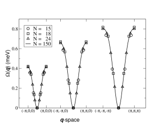
Figure 6: Spin-wave dispersion $\Omega(\vec{q})$ for an ordered, simple cubic superlattice arrangement of Mn spins inside the host semiconductor. Lattices of linear size $N=15,18,24$ and 150, with a total of respectively $125,216,512$ and $125000$ Mn spins are considered. This corresponds to $x=0.0092$ and $p=10\%$. Dispersion is plotted along three linear cuts in the Brillouin zone: $(-\pi,0,0)\rightarrow(\pi,0,0)$, $(-\pi,-\pi,0)\rightarrow(\pi,\pi,0)$ and $(-\pi,-\pi,-\pi)\rightarrow(\pi,\pi,\pi)$.

V.1 Spin-wave density of states

We study the spin-wave density of states for three types of arrangements of the Mn spins inside the host semiconductor. All samples studied correspond to $x=0.0092$ and $p=10\%$. Other parameters are as specified in Section II.

First, we consider fully ordered systems, in which the Mn spins are arranged on a simple cubic superlattice. For $x=0.0092$, the superlattice constant is $a_{L}=3a$. In this case, we can study the spin-wave dispersion and density of states for very large sizes, since we can use directly Eq. (31) to compute the spin-wave frequency $\hbar\omega(\vec{q})$ for each wave-vector $\vec{q}$ inside the Brillouin zone. Spin-wave dispersion obtained along three cuts in the Brillouin zone is shown in Fig. 6. The dispersion has quadratic behavior near the center of the Brillouin zone, as expected from the discussion for an ordered case provided above. The finite-size effects are reasonably small. For the small sizes we used both Eq. (31) and our method to compute the dispersion. The results of the two agree with a relative error of less than $10^{-6}$.

One important aspect to notice is the small range of the spin-wave spectrum, as compared to the AFM exchange $J=15$ meV. This is a consequence of the fact that the Mn spins do not interact directly with one another. Instead, their interaction is mediated by the rather small concentration of charge carriers present.

We compute the density of states (DOS) $\rho(E)$ associated with the spin-wave dispersion for the superlattice case employing the standard method of dividing the Brillouin zone into tetrahedra and linearizing the dispersion (Ref. tetrah, ). The DOS obtained for the lattice with $N=150$, $N_{d}=125,000$ is shown as a dotted line in Fig. 7. We use a logarithmic scale for the energy, and normalize the density of states such that

$$\int_{-\infty}^{\infty}dx\rho(x)=1$$

where $x=\log_{10}(E)$. This convention will be maintained throughout the rest of the paper.

Figure 7: Upper panel: average density of states $\rho(\log_{10}E)$ on a logarithmic scale for systems with $N_{d}=125,216$ and 512 Mn spins in moderately disordered configurations (full lines). Lower panel: average density of states for systems with $N_{d}=125,216$ and 512 Mn spins in strongly disordered configurations (full lines). The dotted line is the spin-wave density of states of a DMS with fully ordered (superlattice) configuration of Mn spins. All samples correspond to $x=0.00924$, $p=10\%$.

In the upper panel of Fig. 7 we also plot the densities of states obtained for moderately disordered configurations with $N_{d}=125,215$ and $512$ Mn spins (full lines). These are configurations in which we place the Mn spins randomly on the FCC Ga sublattice of the host semiconductor, subject to the constraint that the distance between any two spins is larger than $2a$. [In the ordered cubic superlattice, nearest neighbor spin separation is $a_{L}=3a$]. This moderate amount of disorder breaks translational invariance, and the wave-vectors are no longer good quantum numbers. Also, the large degeneracies of the superlattice spectrum are lifted. We computed the spin-wave spectrum for $200$ realizations of the disorder with $N_{d}=125$ spins, 100 realizations with $N_{d}=216$ spins and 50 realizations with $N_{d}=512$ spins. Thus, we have a total of over 21,000 spin-wave energies for each size, and statistics can be comfortably carried out. In particular, from Fig. 7 we see that the DOS histograms corresponding to the three sizes are smooth functions, i.e. the average over disorder is well accounted for. Also, the curves are practically indistinguishable from one another, implying that finite size effects are negligible.

In the lower panel of Fig. 7 we plot the DOS corresponding to fully disordered configurations with $N_{d}=125,215$ and $512$ Mn spins (full lines). These are configurations in which we place the Mn spins randomly on the FCC Ga sublattice of the host semiconductor, with no restrictions (except that each Mn occupies a different site). The number of samples analyzed is the same as in the previous case. Again, the curves show smooth behavior and no finite-size effects. The origin of the peak appearing near $\omega\sim 5~{}$meV will be discussed later.

Before continuing the analysis, we must also point out that the Goldstone modes have been left out in the DOS shown in Fig. 7. The RPA system always has one solution of energy $\omega=0$ (numerically, we find its magnitude to be less that $10^{-14}$), corresponding to $Y_{i}=1/\sqrt{N_{d}}$. This is the Goldstone mode, describing the same overall rotation of all the spins. These Goldstone modes would appear in the DOS as a $\delta(\omega)$ function at $\omega=0$ ($\log_{10}E=-\infty$).

The effect of disorder in the positions of the Mn is reflected in the considerable widening of the DOS (on a logarithmic scale), and rounding of the van Hove singularities of the superlattice DOS, as the amount of disorder increases. More significantly, however, is the substantial enhancement of the DOS at low energies. This behavior is in agreement with the general expectation of the effects of disorder on an energy-band dispersion.

A question of considerable interest concerns the nature of the spin-wave excitations. We know that the ordered superlattice has extended, plane-wave type spin-waves. The general expectation is that disorder will lead to localization, and thus one expects the appearance of localized spin-waves as the disorder increases. One way to characterize the nature of the spin-waves is to compute their Inverse Participation Ratio (IPR), defined as:

$$\rm{IPR}_{\alpha}={{\sum_{i=1}^{N_{d}}\left(Y_{i}^{(\alpha)}\right)^{4}}\over{\left(\sum_{i=1}^{N_{d}}\left(Y_{i}^{(\alpha)}\right)^{2}\right)^{2}}}$$ (33)

For an extended mode $\alpha$ (plane-wave, for instance), we expect that all $Y_{i}^{(\alpha)}$ coefficients are roughly of equal magnitude, since all spins are expected to participate equally in the spin-wave. Then, it follows that for an extended mode $\alpha$, IPR${}_{\alpha}\sim 1/N_{d}$, i.e. it is inversely proportional to the size of the system. On the other hand, in a localized mode $\alpha$, only the spins within the localization volume have non-vanishing values for $Y_{i}^{(\alpha)}$. Thus, it follows that for a localized mode $\alpha$, IPR_α is independent of $N_{d}$. Instead, its value is given by the inverse number of Mn spins participating in the localized mode.

Figure 8: Upper panel: average IPR(E) for systems with $N_{d}=125,216$ and 512 Mn spins in moderately disordered configurations (circles, square and triangles, respectively). Lower panel: same for strongly disordered configurations. All samples correspond to $x=0.00924$, $p=10\%$.

We compute the IPR of the spin-waves in the following manner. As we sweep the frequencies $\omega$ of interest and compute the eigenvalues $\lambda(\omega)$ of the ${\bf M}(\omega)$ matrix on the grid $\delta\omega$, we also compute the corresponding IPR of the eigenvectors ${\bf Y(\omega)}$ (which are normalized to unity). The IPR is a continuous function of $\omega$, and we use linear interpolation to find its value at the spin-wave frequencies $\Omega_{\alpha}$ of interest. Whenever eigenvalues $\lambda(\omega)$ cross, the IPRs are no longer well defined: one can choose any linear combination of the eigenvectors of the degenerate modes, which would lead to different values for the corresponding IPRs. We have checked that these accidental crossings are rather rare (below a few percent) and equally distributed over the entire energy scale. If we exclude all these degenerate cases, we get a DOS which is virtually indistinguishable from the one obtained when these modes are kept. More importantly, we find that modes which cross predominantly have the same nature (either localized or extended). As a result, the ensemble averaged IPR is not sensitive to the precise treatment of these cases.

In Fig. 8 we plot the (geometric) average IPR(E) for the moderate (upper panel) and strong (lower panel) disorder configurations. Again, the Goldstone modes are not shown. We use the geometric mean (i.e., arithmetic mean of the $\log$ values) in order to insure proper weight for the extended modes, with low IPR. For moderate disorder configurations, we see that the spin-wave modes at high energies $E>1$ meV are localized: the values corresponding to the three different sizes collapse on top of one another. This is expected, given the fact that the upper band-edge of the superlattice spectra is just below $E=1$ meV (see Fig. 7). Thus, states of higher energy have been split off the band by disorder, and are expected to be localized. The low-energy part of the band also appears to be localized: while the three curves do not quite meet, the value of the IPR is just below unity, showing that these spin-waves have considerable weight on only one spin (i.e., they correspond to a individual spin-flip). However, for the central part of the spectrum, the spin-waves are extended, with the IPRs for the three sizes clearly distinct and decreasing with increasing $N_{d}$.

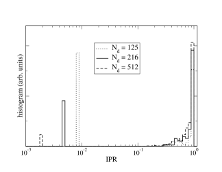
Figure 9: Histogram of the IPR values for all spin-waves (spin flips) of energy $E<5\cdot 10^{-3})$, for $N_{d}=125,216$ and 512. Results are shown only for strong disorder configurations. Except for the low-lying Goldstone modes, the histograms are identical, suggesting only localized modes at these energies.

For the strong disorder configurations, this tendency is even more apparent. The high- and low-energy regions, $E>$ 1 meV, respectively $E<5\cdot 10^{-3}$ meV, contain localized spin-waves: in both limits, the IPR curves collapse on top of one another. The low-energy localized modes are individual spin-flips. The associated $Y_{i}$ are vanishingly small at all sites except one, leading to IPR $\approx 1$. These sites are always situated far apart from all other Mn spins, and the probability to be visited by charge carriers is exponentially small (tailing from far occupied regions). As a result, the Mn spins at these sites are virtually isolated, and their spin excitations are individual spin-flips. The energy for such a spin-flip is equal to $H_{i}$, if one neglects small corrections due to the extremely weak interactions [see Eq. (22) and following discussion].

Histograms of the IPR of all the modes with energies below $E<5\cdot 10^{-3})$ are shown in Fig. 9. Here, we also show the Goldstone modes, which have zero energy, and $IPR=1/N_{d}$. The histograms have been scaled by the total number of modes for all disorder realizations considered for each particular size. Since the number of Goldstone modes exactly equals the number of different realizations of disorder considered, their peaks are in a ratio of roughly 200/100/50 with respect to one another. The main observation is that the histograms for the three sizes are very similar, with a huge peak just below IPR=1. The absence of a dependence on $N_{d}$ confirms that all these modes are localized (except the Goldstone modes, of course).

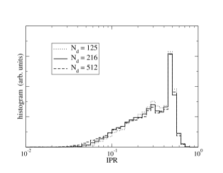
Figure 10: Histogram of the IPR values for all spin-waves (spin flips) of energy $E>10^{-1})$, for $N_{d}=125,216$ and 512. Results are shown only for strong disorder configurations. The histograms are almost identical, suggesting only localized modes at these energies.

The high-energy localized states are of very different nature: their IPR is close to $0.5$, suggesting that it has large contributions from only two sites. Analysis of the $Y_{i}$ values for such modes shows that most of them are associated with nearest-neighbor (n.n.) Mn spins on the FCC Ga sublattice. The characteristic energy for the spin-waves centered on such n.n. sites is just below 5 meV, and this is the feature responsible for the peak appearing in the DOS at these energies (see Fig. 7, lower panel). Careful inspection of the DOS reveals the appearance of smaller peaks at somewhat lower energies (even the DOS for moderate disorder has a small peak at around 2 meV, and its IPR for these modes is close to 0.5). These peaks are associated with excitations of spin-pairs (or larger clusters) with varying separations, but they are not as well defined as the one corresponding to nearest-neighbors spins.

The small clusters of Mn spins giving rise to such modes are always found to be in regions densely populated with charge carriers. Due to their closeness in space, these spins are much more strongly coupled to one another than they are to other spins with which they share charge carriers. This leads to the “resonance-like” character of these modes: either of the spins can be flipped with equal probability. As a result of the strong-coupling, the cost of flipping either spin is high, since it frustrates their FM arrangement. Indeed, the characteristic energy of roughly $J/3$ reflects much stronger coupling than the average one present in the superlattice case. The histogram of the IPR of all modes of energy $E>10^{-1})$ shown in Fig. 10 confirms all these conclusions. We caution that these energies may be substantially modified due to direct antiferromagnetic Mn-Mn exchange (left out in our model) in real systems.

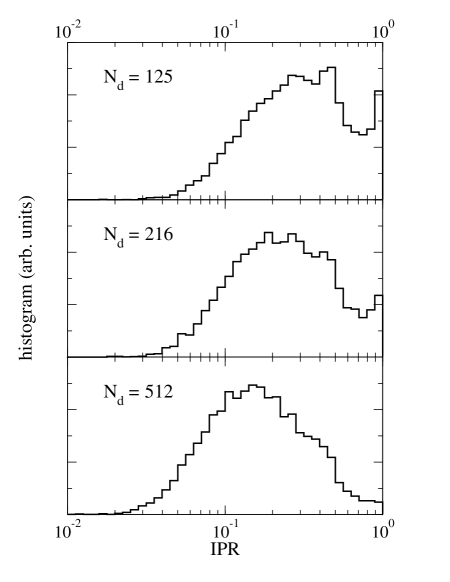
Figure 11: Histogram of the IPR values for all spin-waves (spin flips) of energy $5\cdot 10^{-3})<E<10^{-1})$, for $N_{d}=125$ (upper), 216 (middle) and 512 (lower panel). Results are shown only for strong disorder configurations. With increasing $N_{d}$ the histograms shift to lower values, suggesting that these spin-wave modes are extended.

Finally, the spin-waves at intermediate energies $5\cdot 10^{-3}<E<10^{-1}$ correspond to extended modes. It is rather difficult to establish exactly the “mobility edge” corresponding to the transitions from localized to extended modes at either end, given the rather small system sizes considered here. Thus, we use the values quoted above only as plausible estimates of these boundaries. Clearly, for these energies the average IPR decreases with increasing $N_{d}$ (see Fig. 8). In Fig. 11 we plot the histograms of the IPR for all the modes with energy $5\cdot 10^{-3}<E<10^{-1}$. In this case, size dependence is clearly visible, both in the position of the broad peak maximum as well as in the lower cut-off in IPR value. The position of the maxima scale roughly like $1/N_{d}$. We have attempted both gaussian and lorentzian fits, but neither seems to capture the low-IPR tail properly. In the smaller samples, a second peak appears just below IPR=1. At first sight, this might seem to indicate the existence of a finite density of localized states at these energies as well. However, we believe that this peak is a finite-size effect. Clearly, its amplitude decreases with increasing $N_{d}$ and would vanish in the thermodynamic limit. This is very different from the behavior observed in either of the two localized energy ranges, where the distributions for all sizes are virtually identical (see Figs. 9 and 10). The reason for the appearance of this second peak is simply the restriction IPR $\leq$ 1. As the broad peak moves towards higher values with decreasing $N_{d}$, all the values in the upper tail “bunch” at IPR=1.

One final important observation relates to the absolute values of the IPRs in the extended spin-wave regime. Although scaling with system size is present, the corresponding IPR values are much higher than the ones expected for modes extended over all Mn sites (these values are shown by the positions of the Goldstone modes in Fig. 9, and are well below the cut-offs observed in Fig. 11). This means that in the disordered system, the extended spin-waves are delocalized only over a fraction of the total number of sites. As the amount of disorder increases, this fraction decreases, since IPR averages for the moderate disorder are smaller than IPR averages for full disorder.

These results are consistent with the picture provided by the temperature dependent mean-field study of this model (Ref. MB2, ). There, we concluded that in the disordered system, the (small fraction $p$) of charge carriers are concentrated in a small volume of the sample, where the local Mn concentration is larger than average. As a result, the concentration of charge carriers is strongly enhanced in these regions, and the exchange with the Mn spins inside these regions (which is proportional to the probability of finding charge carriers nearby) is greatly increased, preserving magnetization of these regions up to high temperatures. On the other hand, the Mn spins in the regions devoid of charge carriers are very weakly coupled, and behave as free spins down to very low temperatures. Due to the very inhomogeneous assembly of weakly- and strongly- interacting spins, the magnetization curves have very unusual, concave shapes.

The present study of the spin-waves corroborates the same picture. We find very low-energy, spin-flip like excitations, which are obviously due to the weakly interacting spins, and which are responsible for a very sharp decrease of the magnetization at exponentially small temperatures.MB1 ; MB2 This is is to be contrasted with the behavior of ordered conventional ferromagnets, where at low temperatures only low-energy long-wavelength spin-waves can be excited. Since their phase space is vanishing in the long-wavelength limit ($\sim k^{d}$ in $d$ dimensions), the magnetization of conventional ferromagnets decreases very slowly from its saturation value with increasing temperature, leading to convex upwards magnetization curves.Kaneyoshi

In our model, the extended spin-waves are concentrated around the high-density Mn regions, where the charge carriers mediating the interactions are to be found. This is consistent with the appearance of modes whose IPR, while scaling with the system size, shows modes extended only over a fraction of all system sites. As the amount of disorder decreases all the way to a fully ordered superlattice, the charge carriers are more and more homogeneously spread throughout the sample and the IPR of the extended modes has lower and lower values, as observed from Fig. 8. However, the more homogeneous a sample is, the less the average AFM coupling between the Mn spins and the charge carriers, since the charge carriers have now equal probability of being found anywhere in the sample, instead of being concentrated in a small fraction of the space. This leads to a decrease of the critical temperature $T_{C}$, as observed in both mean-field MB1 and Monte-Carlomalcolm2 analysis. The enhancement of the mean-field $T_{C}$ with increasing disorder is suggested also by the existence of the high-energy localized modes, which show that ferromagnetic alignment will persist in high-density clusters up to very high temperatures. It also suggests that local ferromagnetic fluctuations might be observed well above $T_{C}$.

VI Final Remarks

The aim of this paper is two-fold. First, we demonstrate the accuracy and speed of a new scheme for computing RPA spectra, which allows tackling of systems of much larger sizes than the ones that can be analyzed with the standard RPA formulation. Investigation of large system sizes and averages over many disorder realizations facilitate a clear picture for the problem we are interested in, namely the spectrum and nature of spin-waves of a disordered DMS.

We then demonstrate that disorder can significantly change the spectrum and the nature of the spin-waves. This is likely to lead to important consequences not only as far as magnetic properties are concerned (we have already commented on the fast de-magnetization with increasing temperature, due to low-energy spin-flip modes). More importantly, this may have significant consequences for transport properties as well. For instance, charge carrier spin scattering is likely to be very different in various regions of the sample. Large anomalous Hall effect has been observed in (Ga,Mn)As,Ohnorev but the theory used to interpret it is borrowed from phenomenology relevant to homogeneous ferromagnetic metals. In an inhomogeneous system, some of the accepted ideas might have to be modified or at least verified to still hold true.

References

- (1) H. Ohno, A. Shen, F. Matsukura, A. Oiwa, A. Endo, S. Katsumoto and Y. Iye, Appl. Phys. Lett. 69, 363 (1996).
- (2) T. Hayashi, M. Tanaka, T. Nishinaga, H. Shimada, H. Tsuchiya, Y. Otsuka, J. Cryst. Growth 175, 1063 (1997).
- (3) A. Van Esch, L. Van Bockstal, J. De Boeck, G. Verbanck, A. S. van Steenbergen, P. J. Wellmann, G. Grietens, R. Bogaerts, F. Herlach and G. Borghs, Phys. Rev. B 56, 13103 (1997).
- (4) N. Theodoropoulos, A. F. Hebard, M. E. Overberg, C. R. Abernathy, S. J. Pearton, S. N. G. Chu and R. G. Wilson, Appl. Phys. Lett. bf 78, 3475 (2001); A. F. Hebard, private communication.
- (5) S. Sonoda, S. Shimizu, T. Sasaki, Y. Yamamoto and H. Hori, cond-mat/0108159.
- (6) T. Dietl, A. Haury and Y. M. d’Aubigné, Phys. Rev. B 55, R3347 (1997); M. Takahashi, Phys. Rev. B 56, 7389 (1997); T. Jungwirth, W. A. Atkinson, B. H. Lee and A. H. MacDonald, Phys. Rev. B 59, 9818 (1999); T. Dietl, H. Ohno, F. Matsukura, J. Cibert and D. Ferrand, Science 287, 1019 (2000).
- (7) J. König, H.-H. Lin and A. H. MacDonald, Phys. Rev. Lett. 84, 5628 (2000).
- (8) J. Schliemann, J. Konig and A.H. MacDonald, Phys. Rev. B 64, 165201 (2001).
- (9) A. Chattopadhyay, S. Das Sarma and A. J. Millis, Phys. Rev. Lett. 87, 227202 (2001).
- (10) G. Zarand and B. Janko, cond-mat/0108477.
- (11) S. Sanvito and N. A. Hill, Phys. Rev. B 62, 15553 (2000); S. Sanvito, P. Ordejon and N. A. Hill, Phys. Rev. B 63, 165206 (2001).
- (12) Mona Berciu and R. N. Bhatt, Phys. Rev. Lett. 87, 107203 (2001).
- (13) Mona Berciu and R. N. Bhatt, cond-mat/0111045.
- (14) Malcolm P. Kennett, Mona Berciu and R. N. Bhatt, Phys. Rev. B 65 115308, (2002).
- (15) Malcolm P. Kennett, Mona Berciu and R. N. Bhatt, cond-mat/0203173; R. N. Bhatt, X. Wan, M. P. Kennett and M. Berciu, Comp. Phys. Comm. (in press).
- (16) R. N. Bhatt and Xin Wan, Int. J. Mod. Phys. C 10, 1459 (1999); Xin Wan and R. N. Bhatt, cond-mat/0009161.
- (17) R. N. Bhatt, M. Berciu, M. P. Kennett and X. Wan, J. of Superc. INM 15, 71 (2002).
- (18) J. Okabayashi, A. Kimura, O. Rader, T. Mizokawa, A. Fujimori, T. Hayashi and M. Tanaka, Physica E10, 192 (2001).
- (19) B. Grandidier, J. P. Nys, C. Delerue, D. Stievenard, Y. Higo and M. Tanaka, Appl. Phys. Lett. 77, 4001 (2000).
- (20) D. Basov (private communication).
- (21) J. W. Negele and H. Orland, Quantum Many-Particle Systems (Addison-Wesley Pub. Co., Redwood City, Calif., 1988).
- (22) D. J. Rowe, Nuclear collective motion: models and theory (Methuen, London, 1970).
- (23) J.-P. Blaizot and G. Ripka, Quantum theory of finite systems (MIT Press, Cambridge, Mass., 1986).
- (24) B. Beschoten, P.A. Crowell, I. Malajovich, D. D. Awschalom, F. Matsukura, A. Shen and H. Ohno, Phys. Rev. Lett. 83, 3073 (1999).
- (25) for a review of properties of ferromagnetic III-V semiconductors, see H. Ohno, J. Magn. Magn. Mat. 200, 110 (1999).
- (26) A. K. Bhattacharjee and C. B. á la Guillaume, Solid State Comm. 113, 17 (2000).
- (27) R. N. Bhatt, Phys. Rev. B 24, 3630 (1981).
- (28) Mona Berciu and R. N. Bhatt, cond-mat/0112165.
- (29) Mona I. Berciu, Ph.D. thesis (University of Toronto, 2000).
- (30) G. Lehman and M. Taut, Phys. Stat. Sol. 54, 469 (1972); P. E. Blochl, O. Jepsen and O. K. Andersen, Phys. Rev. B 49, 16223 (1994).
- (31) Uniform magnets as well as metallic alloys are characterized by weak deviations from a universal curve on a versus and plot. [See T. Kaneyoshi, Introduction to Amorphous Magnets, p 56-61 (World Scientific, 1992)].