Glassy Random Matrix Models

Abstract

This paper discusses Random Matrix Models which exhibit the unusual phenomena of having multiple solutions at the same point in phase space. These matrix models have gaps in their spectrum or density of eigenvalues. The free energy and certain correlation functions of these models show differences for the different solutions. Here I present evidence for the presence of multiple solutions both analytically and numerically.

As an example I discuss the double well matrix model with potential $V(M)=-{\mu\over 2}M^{2}+{g\over 4}M^{4}$ where $M$ is a random $N\times N$ matrix (the $M^{4}$ matrix model) as well as the Gaussian Penner model with $V(M)={\mu\over 2}M^{2}-t\ln M$. First I study what these multiple solutions are in the large N limit using the recurrence coefficient of the orthogonal polynomials. Second I discuss these solutions at the non-perturbative level to bring out some differences between the multiple solutions. I also present the two-point density-density correlation functions which further characterizes these models in a new universality class. A motivation for this work is that variants of these models have been conjectured to be models of certain structural glasses in the high temperature phase.

PACS: 02.70.Ns, 61.20.Lc, 61.43.Fs

1 Introduction

Matrix models are known to be of importance in many diverse areas, for example, in quantum chaos, disordered condensed matter systems, two-dimensional quantum gravity, quantum chromodynamics and strings. In the context of the one-matrix models, the models that have been studied correspond to an eigenvalue distribution on a single-cut in the complex plane where the eigenvalue density is non-zero [2]. An obvious generalization is to study a matrix model with a more complicated eigenvalue structure. Here I study a class of models with a single hermitian matrix but with two cuts for the eigenvalue density and point out some unusual features of these models different from the single-cut matrix models. One of the important differences observed in these models is that they have multiple solutions whose effect appears in certain correlation functions. This work suggests the possibility that these multiple solutions may be glassy and hence these models may be useful in describing certain real disordered glassy systems ref. [3, 4].

I study here the matrix model with a double-well potential as well as the Gaussian Penner model where similar results are obtained ref. [5]. In both cases the potential is symmetric about the origin. In addition to the usual symmetric solutions I discuss the symmetry breaking solutions. I study these solutions in the large $N$ limit and then at the non-perturbative level. I also calculate the two-point density-density correlators using orthogonal polynomial methods and methods of steepest descent which strengthens the above observations and classifies the models in a new universality class [6, 7].

2 Notations and Conventions

Let $M$ be a $N\times N$ hermitian matrix. The partition function to be considered is $Z=\int dMe^{-NTrV(M)}$. The Haar measure is given by $dM=\prod_{i=1}^{N}dM_{ii}\prod_{i<j}dM_{ij}^{(1)}dM_{ij}^{(2)}$ where $M_{ij}=M_{ij}^{(1)}+iM_{ij}^{(2)}$; there are $N^{2}$ independent variables. $V(M)$ is a polynomial in $M$: $V(M)=g_{1}M+(g_{2}/2)M^{2}+(g_{3}/3)M^{3}+(g_{4}/4)M^{4}+\ldots$ . $TrV(M)$ and the measure $dM$ are invariant under the change of variables $M\rightarrow M^{\prime}=UMU^{\dagger}$ where $U$ is a unitary matrix. We can use this invariance to express $Z$ as an integral over the eigenvalues $\lambda_{1},\lambda_{2},...,\lambda_{N}$ of $M$. Writing $M=UD^{\prime}U^{\dagger}$ where $D^{\prime}=diag(\lambda_{1},\lambda_{2},.....\lambda_{N})$, the partition function becomes $Z=\int dU\int_{-\infty}^{\infty}\prod_{i=1}^{N}d\lambda_{i}\Delta(\lambda)^{2}e^{-N\sum_{i=1}^{N}V(\lambda_{i})}$ where $\Delta(\lambda)=\prod_{i<j}|\lambda_{i}-\lambda_{j}|$ is the Vandermonde determinant arising from the change of variables. The integration $dU$ is trivial because the integrand is independent of $U$ due to the invariance, and gives a constant factor. By exponentiating the determinant one arrives at the Dyson Gas or Coulomb Gas picture. Thus the partition function is $Z=C\int_{-\infty}^{\infty}\prod_{i=1}^{N}d\lambda_{i}e^{-S(\lambda)}$ where $S(\lambda)=N\sum_{i=1}^{N}V(\lambda_{i})-2\sum_{i\neq j}ln|\lambda_{i}-\lambda_{j}|$, and $C$ is a constant.

This is a system of $N$ particles with coordinates $\lambda_{i}$ on the real line, confined by the potential $V$ and repelling each other with a logarithmic repulsion. The spectrum or the density of eigenvalues $\rho(x)=\langle{1\over N}\sum_{i=1}^{N}\delta(x-\lambda_{i})\rangle$ is, in the large N limit, just the Wigner semi-circle for a quadratic potential. The physical picture is that the eigenvalues try to be at the bottom of the well. But it costs energy to sit on top of each other because of logarithmic repulsion, so they spread. $\rho$ has support on a finite line segment. This continues to be true whether the potential is quadratic or a more general polynomial and only depends on there being a single well though the shape of the Wigner semi-circle is correspondingly modified. For the quadratic potential $V(x)={\mu\over 2}x^{2}$ the density is $\rho(x)={1\over\pi}\sqrt{(x^{2}-a^{2})}$ where $x\in[-a,a]$, and $\rho(x)=0$ elsewhere. The region $[-a,a]$ is said to be the ‘cut’ where $\rho$ has support. The end of the cut is given by $a=\sqrt{2\over\mu}$. See Fig. 1.

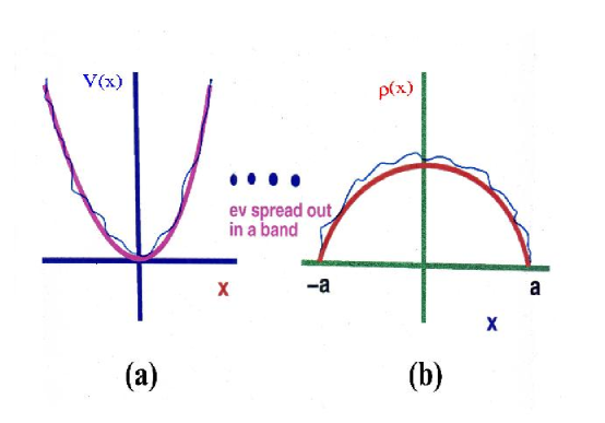
Figure 1: (a). The confining potential (b). The density of eigenvalues

On changing the potential more drastically by having two wells the density can get a support on two disconnected segments ref. [8, 9]. The simplest example is the potential $V(M)={\mu\over 2}M^{2}+{g\over 4}M^{4}$ with $\mu<0,g>0$. When the wells are sufficiently deep, specifically, when $|\mu|>2\sqrt{g}$, the density of eigenvalues is given by

$$\rho(x) = {g\over\pi}x\sqrt{(x^{2}-a^{2})(b^{2}-x^{2})},~{}~{}~{}~{}~{}~{}~{}~{}a\leq x\leq b~{}or~{}-b\leq x\leq-a$$ (2.1)

$$= 0~{}~{}~{}~{}~{}~{}~{}~{}otherwise$$

where $a^{2}={1\over g}[|\mu|-2\sqrt{g}]$ and $b^{2}={1\over g}[|\mu|+2\sqrt{g}]$. The eigenvalues sit in symmetric bands centered around each well. Thus $\rho$ has support on two line segments. As $|\mu|$ approaches $2\sqrt{g}$ from below, $a\rightarrow 0$ and the two bands merge at the origin. For $\mu>-2\sqrt{g}$, the density is

$$\rho(x) = {{gx^{2}}\over\pi}\sqrt{x^{2}-{2\mu\over g}}~{}~{}~{}~{}~{}~{}~{}~{}-\sqrt{2|\mu|\over g}<x<\sqrt{2|\mu|\over g}$$ (2.2)

$$= 0~{}~{}~{}~{}~{}~{}~{}~{}otherwise.$$

The phase diagram and density of eigenvalues for this case is shown in Fig. 2.

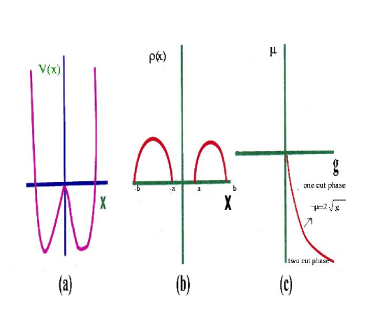
Figure 2: (a). The double-well potential (b). Density of eigenvalues (c). The phase diagram

The simplest way to determine $\rho(z)$ explicitly is to use the generating function $F(z)=\langle{1\over N}Tr{1\over{z-M}}\rangle$. $F(z)$ satisfies a Schwinger-Dyson equation whose solution is $F(z)={1\over 2}[V^{\prime}(z)+\sqrt{\Delta}]$ with $\Delta(z)=V^{\prime}(z)^{2}-4b(z)$ and $b(z)=gz^{2}+\mu+g\langle{1\over N}TrM^{2}\rangle$ (see ref. [5]). The density $\rho(x)$ is then determined by the formula $\rho(z)=-{1\over 2\pi}Im\sqrt{\Delta(z)}$. In what follows I will outline the recurrence coefficient method of the orthogonal polynomials to establish that there exist multiple solutions which give the same free energy $\Gamma$, $F(z)$ and $\rho(z)$ in the large $N$ limit but differ at higher orders. Then I give the results for the two-point correlators (also known as the ‘smoothed’ or ‘long range’ correlators); these tend to different limits as $N$ is taken to infinity along different sequences (odd or even). This property is similar to that suggested in another model of glasses ref. [10].

3 Orthogonal Polynomial Approach

The partition function $Z$ can be rewritten in terms of the orthogonal polynomials $P_{n}$. These are defined as $P_{n}=\lambda^{n}+C^{(n)}_{n-1}\lambda^{n-1}+\ldots+C^{(n)}_{1}\lambda+C^{(n)}_{0}$, where $C^{(n)}_{i}$ are constants, and satisfy the orthogonality conditions $(P_{n},P_{m})=\int_{-\infty}^{\infty}d\lambda e^{-NV(\lambda)}P_{n}(\lambda)P_{m}(\lambda)=h_{n}\delta_{nm}$ . For example: $P_{0}(\lambda)=1$, $P_{1}(\lambda)=\lambda+c^{(1)}_{1}$, $P_{2}(\lambda)=\lambda^{2}+c^{(2)}_{1}\lambda+c^{(2)}_{0}\ldots$. Then the partition function in terms of the orthogonal polynomials is, ref. [11],

$$Z=\int\prod_{i=1}^{N}d\lambda_{i}e^{-N\sum V(\lambda)}\left|\begin{array}[]{ccc}P_{0}(\lambda_{1})&....&P_{0}(\lambda_{N})\\ P_{1}(\lambda_{1})&....&P_{1}(\lambda_{N})\\ .\\ .\\ .\\ P_{N-1}(\lambda_{1})&......&P_{N-1}(\lambda_{N})\\ \end{array}\right|.$$ (3.3)

$Z$ can be expressed in terms of the $h_{n}$’s; $Z=N!h_{0}h_{1}h_{2}.....h_{N-1}.$ For example: in the $N=2$ case, $Z=\int d\lambda_{1}d\lambda_{2}e^{-NV(\lambda_{1})-NV(\lambda_{2})}(P_{0}(\lambda_{1})P_{1}(\lambda_{2})-P_{0}(\lambda_{2})P_{1}(\lambda_{1}))^{2}=h_{0}h_{1}+h_{0}h_{1}=2!h_{0}h_{1}.$

3.1 The Recurrence Coefficients

The $P_{n}$ satisfy recurrence relations, ref. [11],

$$xP_{n}=P_{n+1}+S_{n}P_{n}+R_{n}P_{n-1}$$ (3.4)

where $R_{n}$ and $S_{n}$ are the recurrence coefficients which depend on the potential. These recurrence coefficients are central to our analysis, since the free energy and all correlation functions can be expressed in terms of them. The reason why the $P_{n}$’s satisfy such a simple recursion equation is that $\int xP_{n}P_{n-2}e^{-NV(x)}dx=0$ because $xP_{n-2}$ is a polynomial of degree $n-1$ and can be expressed as a superposition of $P_{n-1},P_{n-2},\ldots P_{0}$. Thus $P_{n-2}$ and lower order polynomials do not appear on the right hand side of the recurrence relation eq. (3.4). It can be shown that $h_{n}=h_{n-1}R_{n}$. Thus the product $h_{0}h_{1}......h_{N-1}=h_{0}(h_{0}R_{1})(h_{0}R_{1}R_{2})......(h_{0}R_{1}...R_{N})=h_{0}^{N}R_{1}^{N-1}R_{2}^{N-2}......R_{N-1}$, hence the free energy $\Gamma=\ln Z=\ln N!+N\ln h_{0}+\sum_{n=1}^{N-1}(N-n)\ln R_{n}.$

To solve for the recurrence coefficients we have three methods based on (i). Integrals, (ii). Recurrence Relations, and (iii). an Effective Potential.

3.1.1 Integrals

The recurrence coefficients can be determined by integrals or moments $I_{n}=\int dxx^{n}e^{-NV(x)}$ as described below. The $P_{n}$’s can be expressed in terms of $R_{n}$ and $S_{n}$ as $P_{n+1}=xP_{n}-S_{n}P_{n}-R_{n}P_{n-1}$, with $P_{0}=1$, $P_{1}=(x-S_{0})$ and $P_{2}=(x-S_{1})(x-S_{0})-R_{1}$ etc. Consider the equation $0=(P_{0},P_{1})=\int dx(x-S_{0})e^{-NV(x)}$, this results in an integral equation for the coefficient $S_{0}$ i.e. $S_{0}={1\over h_{0}}\int dxxe^{-NV(x)}={I_{1}\over I_{0}}.$ As another example the recurrence coefficient $R_{1}$ can be determined as follows. The integral expression for the recurrence coefficient $R_{1}$ is then found from $R_{1}={h_{1}\over h_{0}}$ where $h_{0}=\int dxe^{-NV(x)}=I_{0}$ and $h_{1}=\int dxe^{-NV(x)}P_{1}^{2}(x)=\int dxe^{-NV(x)}(x-S_{0})^{2}=\int dxe^{-NV(x)}(x^{2}-2xS_{0}+S_{0}^{2})=I_{2}-2I_{1}S_{0}+S_{0}^{2}$. Hence $R_{1}={I_{2}\over I_{0}}-({I_{1}\over I_{0}})^{2}$. Similar expressions for all the other recurrence coefficients in terms of integrals can be found.

3.1.2 Recurrence Relations

The recurrence coefficients satisfy recurrence relations that follow from the identities [11]

$$\noindent I.~{}~{}\int dxe^{-NV(x)}P_{n}(x)V^{\prime}(x)P_{n}(x)=0$$ (3.5)

and

$$\noindent II.~{}~{}nh_{n-1}=N\int dxe^{-NV(x)}P_{n}(x)V^{\prime}(x)P_{n-1}(x)$$ (3.6)

I follows from the identity $0=\int P_{n}(x)P^{\prime}_{n}(x)e^{-NV(x)}$ which holds because $P_{n}^{\prime}$, being a linear combination of $P_{n-1}$ and lower order polynomials, is orthogonal to $P_{n}$. II follows from the identity $\int P^{\prime}_{n}(x)P_{n-1}(x)e^{-NV(x)}=nh_{n-1}$.

Let us take the following examples:

(a) $V(x)={\mu\over 2}x^{2}$.
For this potential the recurrence relation I is $0=\mu(P_{n},P_{n+1}+S_{n}P_{n}+R_{n}P_{n-1})=S_{n}h_{n}$, which implies $S_{n}=0$, while the recurrence relation II is $nh_{n-1}=\mu N(P_{n},P_{n}+S_{n-1}P_{n-1}+R_{n-1}P_{n-2})=\mu Nh_{n}$ which implies ${n\over N}=\mu R_{n}$. This determines exactly the recurrence coefficients $S_{n}=0$ and $R_{n}={n\over{N\mu}}$ for this potential.

(b) $V(x)={\mu\over 2}x^{2}+{g\over 4}x^{4}$.
The recurrence relation I is

$$0=\mu S_{n}+g[R_{n+1}(S_{n+1}+2S_{n})+R_{n}(2S_{n}+S_{n-1})+S_{n}^{3}]$$ (3.7)

while II is

$${n\over N}=\mu R_{n}+g(R_{n-1}+R_{n}+R_{n+1})+S_{n}^{2}+S_{n-1}^{2}+S_{n-1}S_{n}.$$ (3.8)

Using the initial values for $R_{0}=0$, $S_{0}$ and $R_{1}$ we can determine $S_{1},R_{2}\ldots$ using the above recurrence relations for the recurrence coefficients.

For this potential we now consider the two cases corresponding to $V$ having one or two wells.

(1) The 1-well case: $\mu>0$, $g>0$.
It follows that $S_{n}=0$, because all $I_{n}$ are zero for odd $n$ whenever $V(x)$ is an even function of $x$. Then the recurrence relation I is trivially satisfied. The recurrence relation II is

$${n\over N}=R_{n}(\mu+g(R_{n+1}+R_{n}+R_{n-1})).$$ (3.9)

Thus $R_{n+1}={n\over{gNR_{n}}}-{\mu\over g}-R_{n}-R_{n-1}$. We determine $R_{1}={I_{2}\over I_{0}}-({I_{1}\over I_{0}})^{2}$ by evaluating $I_{2},I_{1}$ and $I_{0}$ numerically and evaluate $R_{n}$ for $n>1$ using this equation. The result, shown in Fig. 3, suggests that $R_{n}$’s lie on a smooth curve. This curve is analytically determined as follows: For the large $N$ limit we set ${n\over N}=x$ and make the ansatz that $R_{n}$ is a smooth function of $x$ and expand as $R_{n}=R(x)+{1\over N}R_{1}(x)+{1\over N^{2}}R_{2}(x)+\ldots$ . Then to leading order in $N$ eq. (3.9) implies that $x=R(x)[\mu+3gR(x)]$ which is a quadratic equation in $R(x)$ with the solution $R(x)={1\over 6g}[-\mu\pm\sqrt{\mu^{2}+12gx}]$. This fits very well with the numerical evaluation of $R_{n}$ which can be approximated by a smooth curve at large N as shown in Fig. 3.

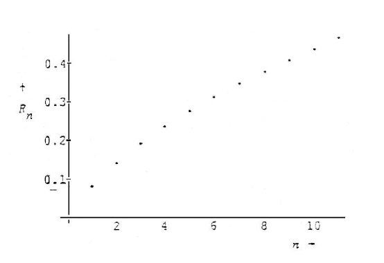
Figure 3: Recurrence coefficients for the single well

The generating function for the single well case is given by (see ref. [5])

$$F(z)=\int_{0}^{1}dx{1\over\sqrt{z^{2}-4R(x)}}.$$ (3.10)

On substituting $R(x)$ in the above equation for the generating function one gets the same answer as that found by the Schwinger-Dyson equation. Eq. (3.10) yields the expression eq. (2.2) for the density of eigenvalues, with a single cut.

(2). The 2-well case, $\mu<0$, $g>0$.
Fig. 4 exhibits a numerical result for $R_{n}$ in this region of phase space which shows that the assumption of a single smooth function describing $R_{n}$ is no longer correct. It suggests the following ansatz for $R_{n}$ at large $N$:

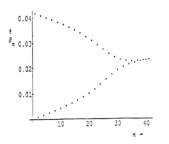
Figure 4: Recurrence coefficients for the double well

For $n\leq\bar{n}$ ( for some $\bar{n}$ to be determined), we have a ‘period-2’ structure:

$$R_{n}=\left\{\begin{array}[]{ll}A_{n}=A(x)+{1\over N}A_{1}(x)+\ldots&for~{}~{}n~{}~{}even\\ B_{n}=B(x)+{1\over N}B_{1}(x)+\ldots&for~{}~{}n~{}~{}odd,\end{array}\right.$$ (3.13)

and for $n>\bar{n}$, we have a ‘period-1’ structure (as for the one-well case):

$$R_{n}=R(x)+{1\over N}R_{1}(x)+\ldots$$ (3.14)

We denote $\bar{x}={{\bar{n}}\over N}$. Substituting eq. (3.13) into eq. (3.9) and equating equal powers of $1\over N$ we get, for $x\leq\bar{x}={\mu^{2}\over 4g}$,

$$A(x) = {1\over 2g}[|\mu|-\sqrt{\mu^{2}-4gx}],$$

$$B(x) = {1\over 2g}[|\mu|+\sqrt{\mu^{2}-4gx}].$$ (3.15)

For $x\geq\bar{x}$, substituting eq. (3.14) into eq. (3.9) we get

$$R(x) = {1\over 6g}[-\mu+\sqrt{\mu^{2}+12gx}].$$ (3.16)

The above analytical result and numerical figure agree very well. Note that $\bar{x}=1$ is the equation for the phase boundary between 1-cut and 2-cut phases (see section 2) in the double well region of parameter space. The generating function in terms of the recurrence coefficients for the two well case is ( see ref. [5] for a derivation )

$$F(z)=\int_{0}^{1}dx{z\over\sqrt{(z^{2}-(A(x)+B(x)))^{2}-4AB}},~{} {\rm if}~{}\bar{x}>1,$$

$$=\int_{0}^{\bar{x}}dx{z\over\sqrt{(z^{2}-(A+B))^{2}-4AB}}+\int_{\bar{x}}^{1}dx{1\over\sqrt{x^{2}-4R(x)}}~{} {\rm if}~{}\bar{x}<1.$$

When $\bar{x}>1$, i.e. in the 2 cut phase, substituting $A,B$ from eq. (3.15), $F(z)={1\over 2}[\mu z+gz^{3}-gz\sqrt{(z^{2}-a^{2})(z^{2}-b^{2})}]$ which is the same as obtained by the Schwinger-Dyson equation. This yields the solution eq. (2.1)for the density of eigenvalues. When $\bar{x}<1$, eqs. (3.15) and (3.16) leads to the one cut solution eq. (2.2).

3.1.3 Effective potential method for determining recurrence coefficients

Numerically we can evaluate the recurrence coefficient by minimizing an effective potential $V_{eff}$ that can be determined from the recurrence relations e.g. for $V(x)=\sigma x+{\mu\over 2}x^{2}+{g\over 2}x^{4}$, the recurrence relations are:

$${n\over N} = R_{n}[\mu+g(R_{n+1}+R_{n}+R_{n-1}+S_{n}^{2}+S_{n-1}^{2}+S_{n-1}S_{n})],$$

$$0 = \sigma+\mu S_{n}+g[R_{n+1}(S_{n+1}+2S_{n})+R_{n}(2S_{n}+S_{n-1})+S_{n}^{3}].$$ (3.18)

It is easy to see that if one defines

$$V_{eff} = \sum_{n=0}^{\infty}\{{-n\over N}lnR_{n}+\mu R_{n}$$ (3.19)

$$+ {g\over 2}(R_{n}^{2}+2R_{n}R_{n+1})+\sigma S_{n}+{\mu\over 2}S_{n}^{2}$$

$$+ {g\over 4}S_{n}^{4}+gR_{n}(S_{n}^{2}+S_{n-1}^{2}+S_{n-1}S_{n})\},$$

then the recurrence relations follow by setting ${{\partial V_{eff}}\over{\partial R_{n}}}=0$ and ${{\partial V_{eff}}\over{\partial S_{n}}}=0$. For $\sigma=0$, setting $S_{n}\equiv 0$ in eq. (3.19) and minimizing with respect to $R_{n}$ yields period 1 or period 2 solutions for $R_{n}$ as shown in figures 3 and 4. However, when $\sigma\neq 0$, $\mu<0,g>0$, (i.e. $V(x)$ has two wells which are asymmetric), then numerical minimization of eq. (3.19) with respect to $R_{n}$ and $S_{n}$ yields a solution of the type displayed in Fig. 5. The figure suggests that the recursion coefficients possibly become chaotic. However, whether they are really chaotic or whether this is only apparently so, requires more detailed numerical work [12]. It would be rather interesting to do this and characterize this chaos and also to understand why the recursion coefficients are so complicated. At any rate, this suggests that it might be interesting to explore solutions of the eq.’s (3.18) for non-zero but small $\sigma$, and see whether at $\sigma=0$, there are alternate solutions ( other than the one with $S_{n}\equiv 0$ discussed earlier ). This indeed turns out to be the case. Fig. 6 shows a numerical solution to eq. (3.18) with $\sigma=0$, obtained by first obtaining solutions for progressively decreasing nonzero values of $\sigma$, and using the solution for a particular value of $\sigma$ as an initial condition to get a solution for the next smaller value of $\sigma$. As seen in Fig. 6, even at $\sigma=0$, we can get a solution with $S_{n}\neq 0$ by this procedure. As we show analytically in the next sections, there is a large family of multiple solutions that exist at $\sigma=0$. One possible explanation for the apparent chaos in Fig. 5 is that a nontrivial mixing between multiple solutions might be occurring.

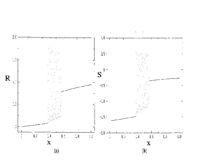
Figure 5: (a). Recurrence coefficients $R_{n}$ for the asymmetric double well (b). Recurrence coefficients $S_{n}$ for the asymmetric double well

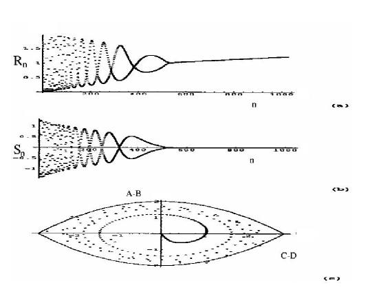
Figure 6: Graphs of recursion coefficients for a spontaneously broken solution of the double-well potential with $N=512,\mu=-2,g=1$ (a). Recurrence coefficients $R_{n}$ and (b). Recurrence coefficients $S_{n}$ after 100000 minimization steps from a random start. (c). Orbit in the A-B vs C-D plane.

4 Multiple Solutions In The Symmetric $M^{4}$ Matrix Model

The simplest way to understand the existence of multiple solutions which appear in these models is to consider the following integral

$$S_{0}={I_{1}\over I_{0}}={{\int_{-\infty}^{\infty}dxxe^{-NV(x)}}\over{\int_{-\infty}^{\infty}dxe^{-NV(x)}}}$$ (4.20)

for $V(x)={\sigma}x+{\mu\over 2}x^{2}+{g\over 4}x^{4}$ with $\mu<0$ and $g>0$, in the limit $\sigma\rightarrow 0$, $V$ has a maximum at $x=0$ and minimum at $x=x^{\pm}=\pm\sqrt{|\mu|\over g}$. The integral $I_{1}$ in eq. (4.20) is zero if we take $\sigma\equiv 0$, and then take $N\rightarrow\infty$ for then the integrand is an odd function. Hence $S_{0}=0$ for $\sigma=0$. However, let us take $\sigma\neq 0$ first, evaluate the integral, in the limit $N\rightarrow\infty$ and then take the limit $\sigma\rightarrow 0$. The integral can be evaluated using the saddle point method. Since for $\sigma\neq 0$, one of the minimas gives dominant contribution, the result is $S_{0}=x^{+}$ as $\sigma\rightarrow 0^{-}$. Thus $S_{0}$ depends upon the order of the limits $N\rightarrow\infty$ and $\sigma\rightarrow 0$.

A more precise way of establishing the presence of multiple solutions in these models is by using the recurrence coefficients; the previous sections have built up the tools that will be used here. Let us relax the condition $S_{n}=0$; we will find that this will be interesting. Consider a period two ansatz for both $R_{n}$ and $S_{n}$. Then

$$R_{n} \rightarrow A_{n},~{}~{}S_{n}\rightarrow C_{n},{\rm for~{}~{}n~{}~{}even,~{}~{}and}$$

$$R_{n} \rightarrow B_{n},~{}~{}S_{n}\rightarrow D_{n},{\rm for~{}~{}n~{}~{}odd}.$$ (4.21)

As before in the large $N$ limit setting $A_{n}$, $B_{n}$, $C_{n}$ and $D_{n}$ to be equal to smooth functions of $x\equiv{n\over N}$, denoted $A$, $B$, $C$, $D$ respectively, one finds that eq.’s (3.18) with $\sigma=0$ reduce to

$$n~{}~{}even~{}~{}x = A[\mu+g(2B+A+C^{2}+D^{2}+CD)]$$

$$n~{}~{}odd~{}~{}x = B[\mu+g(2A+B+C^{2}+D^{2}+CD)]$$

$$n~{}~{}even~{}~{}0 = \mu C+g(B(D+2C)+A(D+2C)+C^{3})$$

$$n~{}~{}odd~{}~{}0 = \mu D+g(A(C+2D)+B(C+2D)+D^{3}).$$ (4.22)

There are four equations and four unknows here but after some work we find that there is only three independent equations. The three independent equations are

$$C+D = 0$$

$$A+B+C^{2} = {-\mu\over g}$$

$$AB = {x\over g}.$$ (4.23)

Thus there is a infinite class of solutions labelled by one function of $x$ in the large $N$ limit. For example, let us consider the two extreme solutions. (i). The ‘symmetric solution’, characterized by $C-D=0$. Then eq. (4.23) implies $C=D=0$, and $A(x)$, $B(x)$ are given by eq. (3.13). This is the same solution as discussed in section 3. (ii). The ‘maximally asymmetric solution’ characterized by, $A-B=0$. Then eq. (4.23) implies $A=B=R=\sqrt{x\over g}$ and $C=-D=[{|\mu|\over g}-\sqrt{4x\over g}]^{1\over 2}$ . The entire infinite class of solutions have the same eigenvalue density and free energy in the large $N$ limit. This can be seen by evaluating the generating function which turns out to be

$$F(z)=\int_{0}^{1}dx{{2z-(C+D)}\over{\sqrt{(z^{2}-z(C+D)-(A+B-CD))^{2}-4AB}}}.$$ (4.24)

Eq. (4.24) contains precisely the same three combinations that are fixed by the recurrence relation eq. (4.23). Therefore independent of which solution is chosen we get the same $F(z)$. Since $F(z)$ determines $\rho$ and the latter determines $\Gamma$ at large $N$, this proves that in the limit $N\rightarrow\infty$ we have an infinite set of solutions of the recurrence relations with the same eigenvalue density and free energy. This demonstrates the presence of multiple solutions from the recurrence coefficient point of view.

5 Non-perturbative Solution

The multiple solutions found above show differences at higher powers of $1\over N$, for example, in the double-scaling limit ref. [9, 13, 14, 15, 16, 17, 18, 19] which I describe in this section. Let us begin by taking the symmetric solution and proceed by expanding the even, odd recurrence coefficients $A,B$ as

$$A_{n} = a_{0}+\epsilon(f_{e}(t)+f_{0}(t))+\epsilon^{2}(r_{e}(t)+r_{0}(t))~{}~{}n~{}~{}even$$

$$B_{n} = a_{0}+\epsilon(f_{e}(t)-f_{0}(t))+\epsilon^{2}(r_{e}(t)-r_{0}(t))~{}~{}n~{}~{}odd$$ (5.25)

where $x={n\over N}=1-\epsilon^{2}t$, $a_{0}={(-\mu)\over 2g}$, and $\epsilon=N^{-1/3}$. Then upon equating equal powers of $\epsilon$, we get $f_{e}=r_{0}=0$, $f_{0}=f(t)$, $r_{e}={{f^{2}-t}\over{4}}$, where the susceptibility is given by $\chi\approx{{f^{2}+t}\over 4}$. $f$ satisfies $f^{\prime\prime}-{1\over 4}f^{3}+{1\over 2}ft=0$ the Painleve II equation.

We then take the asymmetric solution with $A-B\neq 0$, $C-D\neq 0$. On making the following expansion

$$C_{n} = \epsilon g(t)+\epsilon^{2}\ldots$$

$$D_{n} = -\epsilon g(t)+\epsilon^{2}\ldots$$ (5.26)

we get the following coupled equation ref. [16, 17, 18, 19] $f^{\prime\prime}-{1\over 4}f(g^{2}+f^{2})+{1\over 2}ft=0$ and $g^{\prime\prime}-{1\over 4}g(g^{2}+f^{2})+{1\over 2}gt=0.$ If we make the substitution $f=r\cos\theta$, $g=r\sin\theta$ where $r$ and $\theta$ are functions of $t$, then $r$ satisfies a modified Painleve equation

$$\ddot{r}-{1\over 4}r^{3}+{1\over 2}tr-{l^{3}\over r^{3}}=0,~{}~{}r^{2}\dot{\theta}=l=const.$$ (5.27)

The case $l=0$ is the Painleve II equation. The susceptibility $\chi\approx{{f^{2}+g^{2}+t}\over 4}={{r^{2}+t}\over 4}$ and $\chi\approx{3t\over 4}-({{1+l^{2}}\over 4})t^{-2}+\ldots$ which is very different from the symmetric case. Thus the multiple solutions show differences at higher order in $1\over N$.

6 Distinguishing multiple solutions: Correlators, Odd and Even N

Multiple solutions are distinguished by certain correlators. Consider the correlator $\langle TrM~{}~{}TrM\rangle_{c}=\langle TrM~{}~{}TrM\rangle-\langle TrM\rangle^{2}$ where $\langle O\rangle={1\over Z}\int dMe^{-NTrV(M)}O$. It can be shown [5] that $\langle TrM~{}~{}TrM\rangle_{c}=R_{N}$. Since $R_{N}$ depends on the choice of the solution, this demonstrates that the multiple solutions under discussion give rise to different correlation functions in general. In particular note that $R_{N}=A_{N}$ if $N$ is even and $R_{N}=B_{N}$ if $N$ is odd. For the ‘symmetric solution’ $A\neq B$, hence this correlator changes by $O(1)$ as $N$ goes from odd to even. However for the maximally asymmetric solution $A=B$, hence this correlator remains essentially the same as $N$ is changed from odd to even.

Another example of a correlator which distinguishes between the two solutions is

$$\langle TrM~{}~{}TrM~{}~{}TrM\rangle_{c}=R_{N}(S_{N-1}-S_{N}).$$ (6.28)

For the symmetric solution $S_{n}=0$ for all $n$, hence this correlator vanishes. For the asymmetric solution $S_{n}$ is period two and the correlator changes sign while going from odd to even $N$.

The orthogonal polynomial $P_{n}$ can be thought of as a ‘wavefunction’ of a ‘state’ $|n\rangle$ in the ‘coordinate basis’, i.e. $\langle\lambda|n\rangle={P_{n}(\lambda)\over\sqrt{h_{n}}}e^{-{N\over 2}V(\lambda)}$, where $|\lambda\rangle$ are eigenstates of the operator $\hat{M}$. The operator $\hat{M}$ is defined in the basis of states $|n\rangle$ as the matrix

$$\left[\begin{array}[]{ccccc}S_{0}&\sqrt{R_{1}}&0&\ldots\\ \sqrt{R_{1}}&S_{1}&\sqrt{R_{2}}&\ldots\\ 0&\sqrt{R_{2}}&S_{2}&\ldots\\ \end{array}\right],$$ (6.29)

which follows from the recurrence relation satisfied by the orthogonal polynomials eq. (3.9); see ref. [20] for more details. It can be shown that the density of eigenvalues of this matrix in the large $N$ limit is precisely $\rho(\lambda)$. It is therefore of interest to calculate the eigenvalues of this matrix. Since the matrix elements are given by the recurrence coefficients we can determine the eigenvalues numerically (see section (3.1)) from a given solution of the recurrence coefficients. The figures show the location of the eigenvalues for the symmetric solution and the maximally asymmetric solution (see Fig. (7)).

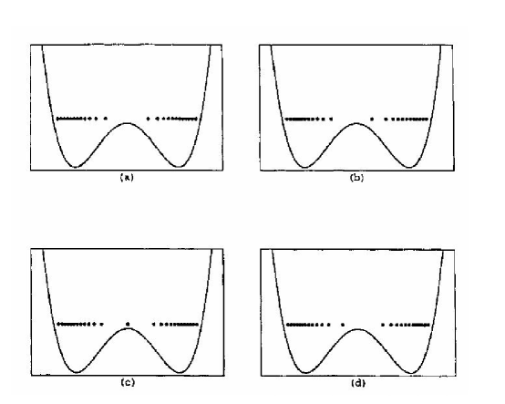
Figure 7: Eigenvalue distribution for even and odd N: (a) N=24, symmetric solution; (b) N=24, asymmetric solution; (c) N=25, symmetric solution; (d) N=25, asymmetric solution.

For $N$ even, half the eigenvalues are in one well and the other half in the other well. While this is true for both solutions the detailed positions are not the same. When $N$ is odd, for the maximally asymmetric solution one extra eigenvalue is located in one of the wells (the well it is located in depends on the sign of $S_{0}$). For the symmetric solution this extra eigenvalue is in the center, thus preserving the symmetry between both wells. This seems to suggest that the bulk effect of the two solutions is the same but they differ by one eigenvalue effects.

Further evidence for the effects of multiple solutions comes from correlation functions of the density operator $\hat{\rho}(x)={1\over N}Tr\delta(x-M)$. The explicit expression for the smoothed two-point correlator for a general 2-cut solution, obtained by the method of steepest descent [21, 22] is

$$4\pi^{2}N^{2}<\hat{\rho}(\lambda)\hat{\rho}(\mu)>_{c}={{\epsilon_{\lambda}\epsilon_{\mu}}\over{\beta\sqrt{|\sigma(\lambda)|}\sqrt{|\sigma(\mu)|}}}~{}~{}~{}~{}~{}~{}~{}~{}~{}~{}$$

$$\left({{\sigma(\lambda)+\sigma(\mu)}\over{(\lambda-\mu)^{2}}}+{{\sigma^{\prime}(\lambda)-\sigma^{\prime}(\mu)}\over{(\lambda-\mu)}}+\lambda^{2}+\mu^{2}-{s\over 2}(\lambda+\mu)+2C\right).$$ (6.30)

Here $\sigma(z)=\prod_{i=1}^{4}(z-a_{i})$, $s=a_{1}+a_{2}+a_{3}+a_{4}$, (the support of the eigenvalues consists of the two segments $[a_{1},a_{2}]$ and $[a_{3},a_{4}]$), $\epsilon_{\lambda}=+1~{}~{}{\rm for}~{}~{}\lambda\in[a_{3},a_{4}],\epsilon_{\lambda}=-1~{}~{}{\rm for}~{}~{}\lambda\in[a_{1},a_{2}]$ and $\beta=1,2,4$ depending on whether $M$ the matrix is real orthogonal, hermitian or self-dual quartonian. $C$ is an undetermined constant in this method. It turns out that the same correlator can be calculated using other methods, which yield different values of $C$. For example in [22] we obtained an asymptotic form of $P_{n}(x)$ for the symmetric double well potentials for $n$ close to $N$. Using this form of $P_{n}$ (which corresponds to the ‘symmetric solution’), we found the smoothed $<\hat{\rho}\hat{\rho}>_{c}$ given by eq. (6.30), with $C=(-1)^{N}$, (the origin of this nontrivial $N$ dependence, also observed in [23], is explained in [24]). On the other hand in ref. [25], this correlator was calculated by the loop equation method starting from an asymmetric $V$ and taking the limit of a symmetric potential where $C$ was found to be $-{1\over 2}\{(a^{2}+b^{2})-(a+b)^{2}[{E(k)\over K(k)}]\}$ where $E(k)$ and $K(k)$ are complete elliptic integrals of the first and second kind and $k={{2\sqrt{ab}}\over{(a+b)}}$. We conjecture that different values of $C$ corresond to different solutions of the recurrence coefficients.

In this section, we have shown the multiple solutions discussed in section 4 give rise to different correlation functions. An interesting feature of the solutions is that there is a nontrivial $N$ dependence which survives in the large $N$ limit. In particular, for the symmetric solution we have shown a difference between odd and even $N$ in the thermodynamic limit. This is reminiscent of the behaviour in a model for glasses [10].

7 The connection of random matrix models with a simple model of structural glasses

This section is concerned with building up a connection with the study of structural glasses in the high temperature phase, starting from the work of ref. [3, 4]. The hamiltonian $H={1\over n}\sum_{a\neq b}(s^{a}.s^{b})^{p}$ corresponds to $n$ particles moving in an $N$-dimensional space, in the limit $n,N\rightarrow\infty$. The coordinates of the particles are $s^{a}=(s^{a}_{1}......s^{a}_{N})$ and $a=1......n$. In the ‘spherical’ case the particles are constrained to move on the surface $|s^{a}|^{2}=N$, for all $a$. In the ‘Ising’ case they occupy only the vertices of a hypercube $s^{a}_{i}=\pm 1$.

The corresponding partition function is $Z=e^{\beta N^{2}}Tr_{\{s\}}exp[-{\beta\over{\alpha N}}tr(S^{\dagger}SS^{\dagger}S)]$ where $S$ is the $N\times n$ rectangular matrix of elements $s_{i}^{a}$, and $Tr_{\{s\}}$ runs over either the spherical or the Ising measure. Here $n=\alpha N$ with $\alpha\geq 1$. Using the large $N$ equivalence with the global constraint one gets

$$Z_{sph}\approx e^{\beta N^{2}}\int d\mu\int\prod_{i=1}^{N}dx_{i}exp\left(-N^{2}{{\beta\mu}\over 2}-\beta E[x]\right)$$ (7.31)

The $x_{i}\sqrt{N}$ are the “diagonal” values of $S$ in its canonical form and $E[x]\equiv N\sum_{i=1}^{N}V(x_{i})-{1\over 2\beta}\sum_{i\neq j}ln|x_{i}^{2}-x_{j}^{2}|$ where $x=(x_{1},x_{2},...,x_{N})$ and $V(x)$ is given by

$$V(x)=\left({1\over\alpha}x^{4}-{\mu\over{2\alpha}}x^{2}-{(\alpha-1)\over\beta}\ln|x|\right).$$ (7.32)

This potential has the form of the generalized Penner model. I show briefly (see ref. [5]) that a very closely related model that can be exactly solved, the Gaussian Penner model, has 2 cuts and multiple solutions. So the above model which is a variant of the Penner model with two cuts, is also conjectured to have multiple solutions.

The potential for a general Penner model is $V(M)=V_{0}(M)-t\ln M$, where $V_{0}$ is a polynomial. If $V_{0}(M)={1\over 2}\mu M^{2}$ the model is the Gaussian Penner model where we can re-write $\ln M={1\over 2}\ln M^{2}$. This has $Z_{2}$ symmetry and the potential is a double well with eigenvalues distributed in disconnected segments. The partition function for the Gaussian Penner model in terms of its eigenvalues $x_{i}$ is [26]

$$Z=\int\prod dx_{i}exp[-E(x)]$$ (7.33)

where $E[x]=N\sum_{i=1}^{N}V(x_{i})-2\sum_{i\neq j}\ln|x_{i}-x_{j}|$

$$V(x)=N\left({\mu\over 2}x^{2}-t\ln|x|\right).$$ (7.34)

This potential is similar to that of eq. (7.32), in that it has a double-well potential involving $ln|x|$. I will show explicitly that this has multiple solutions. We consider the situation for $t>0$.

The recurrence relations for a general Penner model reduce to

$${n\over N} = \sqrt{R_{n}}\langle n-1|V_{0}^{\prime}(\hat{M})|n\rangle-t\sqrt{R_{n}}\langle n-1|\hat{M}^{-1}\|n\rangle$$

$$0 = \langle n|V^{\prime}_{0}(\hat{M})\|n\rangle-t\langle n|\hat{M}^{-1}|n\rangle$$ (7.35)

Denoting $W_{n}=\sqrt{R_{n}}\langle n-1|V_{0}^{\prime}(\hat{M})\|n\rangle$ and $Y_{n}=\langle n|V_{0}^{\prime}(\hat{M})\|n\rangle$, for the Gaussian Penner model $W_{n}=\mu R_{n}$ and $Y_{n}=\mu S_{n}$. We can consider as in section 4, a period-2 ansatz for $R_{n}$ and $S_{n}$ which leads to four equations but again only three independent equations:

$$C+D = 0$$

$$A+B-CD = {{2x+t}\over\mu}$$

$$AB = {{x(x+t)}\over\mu^{2}}.$$ (7.36)

Thus there is an infinite class of solutions labelled by one function of $x$ in the large $N$ limit. For the ‘symmetric solution’: $C=D=0$ and $A={x\over\mu},~{}~{}B={{x+t}\over\mu}$ while the maximally asymmetric solution: $A=B={1\over\mu}\sqrt{x(x+t)}$ and $C^{2}={1\over\mu}[(2x+t)-2\sqrt{x(x+t)}].$ Once again eq. (7.36) fixes the same combinations which appear in the generating function of the Gaussian Penner model. Thus in the large $N$ limit the eigenvalue density and free energy are identical for the full infinite class of solutions satisfying eq. (7.36).

For the symmetric solution $\langle n|\hat{M}^{-1}|n\rangle=0$ by $Z_{2}$ symmetry and $S_{n}=0$, thus eq. (7.35) yields $R_{n}={n\over{\mu N}}$ for $n$ even and $R_{n}={n\over\mu N}+{t\over\mu}$ for $n$ odd. This is an exact solution, hence the exact free energy may be found to be $\Gamma=\sum_{k=1}^{N/2-1}k\log[(2k+\mu+1)(2k+\mu-1)],$ where $t=-1+{\mu\over N}$. Expanding in powers of $\mu$ we get

$$\Gamma={1\over 4}\mu^{2}\log\mu+{1\over 12}\log\mu\ldots.$$ (7.37)

Note that the coefficient of the second term $\log\mu$ is $\chi_{1}={1\over 12}$ which corresponds to the first subleading correction in the $1\over N$ expansion. For the maximally asymmetric solution in the double scaled limit $R_{n}\approx{\Gamma(1/2(N-n+\mu+3/2))\over\Gamma(1/2(N-n+\mu+1/2))}$, and the free energy is $\Gamma=\sum_{k=1}^{N/2-1}k\log[(2k+\mu+1/2)(2k+\mu-1/2)]+\ldots$ . On expanding in powers of $\mu$ the free energy is

$$\Gamma={1\over 4}\mu^{2}\log\mu-{5\over 48}\log\mu\ldots$$ (7.38)

The coefficient of the second term is ${5\over 48}$. Here in the Gaussian Penner model we see that though the symmetric and maximally asymmetric solutions give the same answer in the large $N$ limit, the free energies are very different at higher order. This establishes that in the Gaussian Penner model multiple solutions are present which give the same free energy in the large $N$ limit but differ at higher orders. As in section 7, certain correlation functions will be different for these solutions since they depend upon the recursion coefficents.

The potential $V(x)$ for the glass model discussed in the high temperature region is qualitatively similar to the $V(x)$ for the Gaussian Penner model in that both have double wells. This feature is the same for the $M^{4}$ model discussed in earlier sections. Since these later models which have two cuts in their eigenvalue density have been shown to have multiple solutions, it is conjectured here that the glass model described above in the high temperature phase should also have multiple solutions. It would be useful to show this explicitly in the future.

More recent work [27] suggests that the number of multiple solutions grows exponentially with $N$. This gives further support for glassy behavior in these gapped random matrix models.

8 Conclusions

To conclude, ample evidence has been provided for the existence of multiple solutions in random matrix models with gaps. First a simple motivation for the presence of multiple solutions is given and then made more precise using the recurrence coefficients of the orthogonal polynomials of the system. Further, numerical evidence is given for the existence of multiple solutions in this context. In the large $N$ limit the free energy, generating function and density are the same. Differences between the multiple solutions are seen in the free energy at higher orders in $1\over N$ as well as in correlation functions.

Connections with the high temperature phase of structural glasses have been made to matrix models [3, 4]. These are a variant of the Penner model with two-cuts. A simpler model, the Gaussian Penner model, with disconnected segments is shown to have these unusual multiple solutions as well. Hence the matrix models with gaps with connections to glass models are likely to have this unusual property. The ruggedness of the landscape needs to be studied. It would be nice to be able to cast these models in the replica framework but this remains a difficult task at this point, as the Hubbard-Stratanovich transformations which are technically needed for the Gaussian random matrix models ref. [28] are not available here for the simple $M^{4}$ and the Gaussian Penner model or any other gapped random matrix models. This is a future goal in this problem.

9 Acknowledgments

I thank E. Brézin, R. C. Brower, C. Dasgupta, S. Jain and C-I Tan for encouragement and collaborations. Thanks to S. Jain for critical reading of the manuscript. I would like to thank the Raman Research Institute, Santa Fe Institute and the Abdus Salam International Center for Theoretical Physics for hospitality and facilities where part of this work was done.

References

- [1]
- [2] M. L. Mehta Random matrices (Academic Press, 1991), T. Guhr, A. Mueller-Groeling and H. A. Weidenmueller, Phys. Rep. 299, (1998), 189.
- [3] L. F. Cugliandolo, J. Kurchan, G. Parisi and F. Ritort, Phys. Rev. Lett. 74 (1995) 1012.
- [4] G. Parisi, Statistical Properties of Random Matrices and the Replica method, cond-mat/9701032.
- [5] R. C. Brower, N. Deo, S. Jain and C. I. Tan, Nucl. Phys. B405 (1993) 166.
- [6] J. Ambjorn, J. Jurkiewicz and Yu. M. Makeenko, Phys. Lett. B251 (1990) 517.
- [7] E. Brézin and A. Zee, Nucl. Phys. B402 (1993) 613.
- [8] Y. Shimamune, Phys. Lett. B108 (1982) 407; G.M. Cicuta, L. Molinari and E. Montaldi, Mod. Phys. Lett. A1 (1986) 125; J. Phys. A23 (1990) L421; J. Jurkiewicz, Phys. Lett. 245 (1990) 178; G. Bhanot, G. Mandal and O. Narayan, Phys. Lett. B251 (1990) 388.
- [9] K. Demeterfi, N. Deo, S. Jain and C-I Tan, Phys. Rev. D42 (1990) 4105.
- [10] Marinari E., Parisi G. and Ritort F. J. Phys. A:Math.Gen.27 (1994) 7615,7647.
- [11] Bessis D., Commun. Math. Phys. 69 147 (1979); Bessis D., Itzykson C. and Zuber J. B., Adv. Appl. Math. 1 109 (1980).
- [12] O. Lechtenfeld, R. Ray and A. Ray, Intern. J. Mod. Phys. A6 (1991) 4491; M. Sasaki and H. Suzuki, Phys. Rev. D43 (1991) 4015; O. Lechtenfeld, Intern. J. Mod. Phys. A7 (1992) 2335; D. Senechal, Intern. J. Mod. Phys. A7 (1992) 1491.
- [13] M. Douglas, N. Seiberg and S. Shenker, Phys. Lett. B244 (1990)381.
- [14] C. Crnkkovic and G. Moore, Phys. Lett. B257 (1991)322.
- [15] P. Mathieu and D. Senechal, Mod. Phys. Lett. A6 (1991) 819.
- [16] C. Nappi, Mod. Phys. Lett. A5 (1990) 2773.
- [17] P. M. S. Petropoulos, Phys. Lett. B261 (1991) 402.
- [18] C. Crnkovic, M. Douglas and G. Moore, Yale and Rutgers preprint YCPT-P25-91, RU-91-36.
- [19] T. Hollowood, L. Miramontes, A. Pasquinucci and C. Nappi, Nucl. Phys. B373 (1992) 247.
- [20] V.A.Kazakov, Mod. Phys. Lett. A4 (1989) 2125; D. Gross and A.A.Migdal, Nucl. Phys. B340 (1990) 333; H. Neuberger, Nucl. Phys. B352 (1991) 689; S. Dalley, C. Johnson and T. Morris, Phys. Lett. B262 (1991) 81; M. Bowick and E. Brezin, Phys. Lett. B268 (1991) 21.
- [21] N. Deo, Nucl. Phys. B504 (1997) 609.
- [22] E. Brézin and N. Deo, Phys. Rev. E 59 (1999) 3901.
- [23] E. Kanzieper and V. Freilikher, Phys. Rev. E 57 (1998) 6604.
- [24] G. Bonnet, F. David and B. Eynard, J. Phys. A33 (2000) 6739.
- [25] G. Akemann and J. Ambjorn, J. Phys. A29 (1996) L555, G. Akemann, Nucl. Phys. B482 (1996) 403 and Nucl. Phys. B507 (1997) 475.
- [26] J. Harer and D. Zagier, Invent. Math. 85 (1986) 457; R.C. Penner, Bull. Amer. Math. Soc. 15 (1986) 73; J. Diff. Geom. 27 (1988) 35; J. Distler and C. Vafa, Mod. Phys. Lett. A6 (1991) 259; C-I Tan, Mod. Phys. Lett. A6 (1991) 1373; C-I Tan, Phys. Rev. D45 (1992) 2862; S. Chaudhuri, H. Dykstra and J. Lykken, Proc. XXth Int. Conf. on Differential Geometric Methods in Theoretical Physics, New York, June 1991.
- [27] N. Deo, S. Jain and E. Brézin, Tapping and Counting in Glassy Random Matrix Models, Preprint in Preparation.
- [28] A. Kamenev and M. Mézard, Wigner-Dyson Statistics from the Replica Method, cond-mat/9901110; Level Correlations in Disordered Metals: the Replica Sigma-model, cond-mat/9903001.