Transport coefficients of $d$-dimensional inelastic Maxwell models

Abstract

Due to the mathematical complexity of the Boltzmann equation for inelastic hard spheres, a kinetic model has recently been proposed whereby the collision rate (which is proportional to the relative velocity for hard spheres) is replaced by an average velocity-independent value. The resulting inelastic Maxwell model has received a large amount of recent interest, especially in connection with the high energy tail of homogeneous states. In this paper the transport coefficients of inelastic Maxwell models in $d$ dimensions are derived by means of the Chapman–Enskog method for unforced systems as well as for systems driven by a Gaussian thermostat and by a white noise thermostat. Comparison with known transport coefficients of inelastic hard spheres shows that their dependence on inelasticity is captured by the inelastic Maxwell models only in a mild qualitative way. Paradoxically, a much simpler BGK-like model kinetic equation is closer to the results for inelastic hard spheres than the inelastic Maxwell model.

1 Introduction

As is known, the Boltzmann equation for elastic hard spheres is in general very complicated to deal with, so that explicit results are usually restricted to small deviations from equilibrium [1]. In order to explore a wider range of situations, the direct simulation Monte Carlo (DSMC) method [2, 3] can be used as an efficient tool to solve numerically the Boltzmann equation. From a theoretically oriented point of view, another fruitful route consists of replacing the detailed Boltzmann collision operator by a simpler collision model, e.g. the BGK model [4], that otherwise retains the most relevant physical features of the true collision operator [5]. Several exact solutions of the nonlinear BGK model kinetic equation [6] have proven to agree rather well with DSMC results for the Fourier flow [7], the uniform shear flow [8], the Couette flow [9, 10] and the Poiseuille flow [11]. In a third approach, the mathematical structure of the Boltzmann collision operator is retained, but the particles are assumed to interact via the repulsive Maxwell potential (inversely proportional to the fourth power of the distance) [12]. For this interaction model, the collision rate is independent of the relative velocity of the colliding pair and this allows for a number of nice mathematical properties of the collision operator [13, 14, 15]. Since many interesting transport properties (both linear and nonlinear), once properly nondimensionalized, are only weakly dependent on the interaction potential, exact results derived from the Boltzmann equation for elastic Maxwell molecules [16] are often useful for elastic hard spheres [8] and even Lennard-Jones particles [17, 18]. Quoting Ernst and Brito [19, 20], one can say that “Maxwell molecules are for kinetic theory what harmonic oscillators are for quantum mechanics and dumb-bells for polymer physics.”

The prototype model for the description of granular media in the regime of rapid flow consists of an assembly of (smooth) inelastic hard spheres (IHS) with a constant coefficient of normal restitution $\alpha$ [21]. In the low density limit spatial correlations can be neglected. If, in addition, the pre-collision velocities of two particles at contact are assumed to be uncorrelated (molecular chaos assumption), the velocity distribution function obeys the Boltzmann equation, modified to account for the inelasticity of collisions [22, 23].

Needless to say, all the intricacies of the Boltzmann equation for elastic hard spheres are inherited and increased further by the Boltzmann equation for IHS, the latter introducing the coefficient of normal restitution $0\leq\alpha<1$ in the collision rule. Therefore, it is not surprising that the three alternative approaches mentioned above for elastic collisions, namely the DSMC method, the model kinetic equation and the Maxwell model, have been extended to the case of inelastic collisions as well. As for the DSMC method, its extension from the original formulation for elastic collisions ($\alpha=1$) [2, 3] to $\alpha<1$ is straightforward [24]. The generalization of the familiar BGK model kinetic equation is less evident, but a physically meaningful proposal has recently been made [25]. This model has proven to yield results in good agreement with DSMC data for the simple shear flow problem [26, 27] and for the nonlinear Couette flow [28]. Following the third route, the collision rate of a colliding pair of inelastic spheres, which is proportional to the magnitude of the relative velocity, is replaced by an average constant collision rate [29]. The resulting collision operator shares some of the mathematical properties of that of elastic Maxwell molecules and so this model is referred to as pseudo-Maxwellian model [29] or, as will be done here, inelastic Maxwell model (IMM) [19]. The Boltzmann equation for IMM has received a large amount of interest in the last few months [19, 20, 29, 30, 31, 32, 33, 34, 35, 36, 37, 38, 39, 40].

The IMM is worth studying by itself as a toy model to exemplify the non-trivial influence of the inelastic character of collisions on the physical properties of the system. On the other hand, its practical usefulness is strongly tied to its capability of mimicking the relevant behaviour of IHS. A common property of the Boltzmann equation for IHS and IMM is that both have homogeneous solutions exhibiting high energy tails overpopulated with respect to the Maxwell–Boltzmann distribution. But this general qualitative agreement fails at a deeper level. More specifically, in the homogeneous cooling state the (reduced) velocity distribution function $\widetilde{f}(\mathbf{c})$, where $\mathbf{c}$ is the velocity relative to the thermal velocity, decays asymptotically as $\ln\widetilde{f}\sim-c$ in the case of IHS [41, 42] and as $\ln\widetilde{f}\sim-\ln c$ in the case of IMM [19, 20, 33, 35]. Analogously, in the steady homogeneous state driven by a white noise forcing, the asymptotic behaviour is $\ln\widetilde{f}\sim-c^{3/2}$ in the case of IHS [42], while $\ln\widetilde{f}\sim-c$ for IMM [37]. Of course, these discrepancies in the limit of large velocities do not preclude that the the IMM may characterize well the “bulk” of the velocity distribution of IHS, as measured by low degree moments. In a nonequilibrium gas, the physically most relevant moments (apart from the local number density $n$, flow velocity $\mathbf{u}$ and granular temperature $T$) are those associated with the fluxes of momentum and energy. If the gradients of $n$, $\mathbf{u}$ and $T$ are weak enough, the fluxes are linear combinations of the gradients, thus defining the transport coefficients (e.g. the shear viscosity and the thermal conductivity) as nonlinear functions of the coefficient of restitution. These transport coefficients have been obtained by an extension of the Chapman–Enskog method [1] from the Boltzmann equation for IHS [43, 44, 45, 46]. To the best of my knowledge, they have not been derived for IMM. The major aim of this paper is to carry out such a derivation and perform a detailed comparison between the transport coefficients for IMM and IHS.

The plan of the paper is as follows. In Sec. 2 the Boltzmann equation for IMM in $d$ dimensions is introduced. The model includes an average collision frequency $\omega$ that can be freely fitted to optimize the agreement with IHS. In the absence of any external forcing the energy balance equation contains a sink term due to the collisional energy dissipation. This term is represented by the cooling rate $\zeta$, that is proportional to the collision frequency $\omega$ and to the inelasticity parameter $1-\alpha^{2}$. The sink term can be compensated for by an opposite source term representing some sort of external driving. For concreteness, two types of driving are considered: a deterministic force proportional to the (peculiar) velocity (Gaussian thermostat) and a stochastic “kicking” force (white noise thermostat). The corresponding homogeneous solutions are analyzed in Sec. 3, where the fourth cumulant (or kurtosis) of the velocity distribution is exactly obtained, being insensitive to the choice of $\omega$. Comparison with the fourth cumulant of IHS shows significant deviations, especially in the case of the homogeneous cooling state (which is equivalent to the homogeneous steady state driven by the Gaussian thermostat). The Chapman–Enskog method is applied in Sec. 4 to get the transport coefficients of IMM in the undriven case, as well as in the presence of the Gaussian thermostat and the white noise thermostat. For undriven systems with $d\leq 3$, it is found that the thermal conductivity diverges at $\alpha=(4-d)/3d$ and becomes negative for $\alpha<(4-d)/3d$, irrespective of the choice of $\omega$. A critical comparison with the transport coefficients of IHS is carried out in Sec. 5. The free parameter $\omega$ is fixed by the criterion that the cooling rate of IMM be the same as that of IHS (in the local equilibrium approximation). The comparison shows that the IMM retains only the basic qualitative features of the $\alpha$–dependence of the IHS transport coefficients. The best agreement takes place in the case of the white noise thermostat, where the influence of the inelasticity on the values of the transport coefficients is rather weak. Quite surprisingly, the transport coefficients predicted by the much simpler BGK-like model [25] are in general much closer to the IHS ones than those obtained from the IMM. The paper ends in Sec. 6 with some concluding remarks.

2 Inelastic Maxwell models

The Boltzmann equation for inelastic Maxwell models (IMM) [20, 29, 31] can be obtained from the Boltzmann equation for inelastic hard spheres (IHS) by replacing the term $|\mathbf{g}\cdot\widehat{\bm{\sigma}}|$ in the collision rate (where ${\bf g}={\bf v}_{1}-{\bf v}_{2}$ is the relative velocity of the colliding pair and $\widehat{\bm{\sigma}}$ is the unit vector directed along the centres of the two colliding spheres) by an average value proportional to the thermal velocity $v_{0}=\sqrt{2T/m}$ (where $T$ is the granular temperature and $m$ is the mass of a particle). The resulting Boltzmann equation is [20]

$$(\partial_{t}+{\bf v}_{1}\cdot\nabla+\mathcal{F})f({\bf r},{\bf v}_{1};t) = \frac{\omega({\bf r},t;\alpha)}{n({\bf r},t)\Omega_{d}}\int\d\widehat{\bm{\sigma}}\int\d{\bf v}_{2}\left(\alpha^{-1}\widehat{b}^{-1}-1\right)$$ (1)

$$\times f({\bf r},{\bf v}_{1};t)f({\bf r},{\bf v}_{2};t)$$

$$\equiv J[{\bf r},{\bf v}_{1};t|f],$$

where $n$ is the number density, $\omega(\alpha)\propto nT^{1/2}$ is an effective collision frequency, $\Omega_{d}=2\pi^{d/2}/\Gamma(d/2)$ is the total solid angle in $d$ dimensions, $\alpha<1$ is the coefficient of normal restitution, and $\widehat{b}$ is the operator transforming pre-collision velocities into post-collision ones:

$$\widehat{b}{\bf v}_{1,2}={\bf v}_{1,2}\mp\frac{1+\alpha}{2}({\bf g}\cdot\widehat{\bm{\sigma}})\widehat{\bm{\sigma}}.$$ (2)

Equations (1) and (2) represent the simplest version of the model, since the collision rate is assumed to be independent of the relative orientation between the unit vectors $\widehat{\mathbf{g}}$ and $\widehat{\bm{\sigma}}$ [20]. In a more realistic version, the collision rate has the same dependence on the scalar product $\widehat{\mathbf{g}}\cdot\widehat{\bm{\sigma}}$ as in the case of hard spheres. The corresponding Boltzmann equation can be proved to be equivalent to Eq. (1), except that the operator $\widehat{b}$ must be replaced by [29, 31]

$$\widehat{b}{\bf v}_{1,2}=\frac{1}{2}\left({\bf v}_{1}+\mathbf{v}_{2}\right)\pm\frac{1-\alpha}{4}\mathbf{g}\pm\frac{1+\alpha}{4}g\widehat{\bm{\sigma}}.$$ (3)

Both versions of the model yield similar results in issues as delicate as the high energy tails [20, 37]. For the sake of simplicity, henceforth I will restrict myself to the version of the model corresponding to the conventional collision rule (2).

The collision frequency $\omega(\alpha)$ is a free parameter of the model. Its detailed $\alpha$–dependence can be determined by optimizing the agreement between the results derived from Eq. (1) and those derived from the original Boltzmann equation for IHS. Of course, the choice of $\omega(\alpha)$ is not unique and may depend on the property of interest.

In Eq. (1), $\mathcal{F}$ is an operator representing the action of a possible external driving. This operator is assumed to preserve the local number and momentum densities, i.e.,

$$\int\d\mathbf{v}\,\mathcal{F}f({\bf r},{\bf v};t)=\int\d\mathbf{v}\,\mathbf{v}\mathcal{F}f({\bf r},{\bf v};t)=0.$$ (4)

On the other hand, in general the external driving gives rise to an energy source term

$$\gamma(\mathbf{r},t)=-\frac{m}{dn(\mathbf{r},t)T(\mathbf{r},t)}\int\d\mathbf{v}\,{V}^{2}\mathcal{F}f({\bf r},{\bf v};t),$$ (5)

where

$$T(\mathbf{r},t)=\frac{m}{dn(\mathbf{r},t)}\int\d\mathbf{v}\,{V}^{2}f({\bf r},{\bf v};t)$$ (6)

defines the granular temperature and $\mathbf{V}=\mathbf{v}-\mathbf{u}$ is the peculiar velocity,

$$\mathbf{u}(\mathbf{r},t)=\frac{m}{n(\mathbf{r},t)}\int\d\mathbf{v}\,\mathbf{v}f({\bf r},{\bf v};t)$$ (7)

being the flow velocity. A possible external driving corresponds to a deterministic nonconservative force of the form $\frac{1}{2}m\gamma\mathbf{V}$ [37, 47]. It has been widely used to generate nonequilibrium steady states in the context of molecular fluids and can be justified by Gauss’s principle of least constraints [48, 49]. The operator $\mathcal{F}$ describing this force is

$$\mathcal{F}f(\mathbf{r},\mathbf{v};t)=\frac{1}{2}\gamma(\mathbf{r},t)\frac{\partial}{\partial{\bf v}}\cdot\left[\mathbf{V}f(\mathbf{r},\mathbf{v};t)\right].$$ (8)

The most commonly used type of driving for inelastic particles consists of a stochastic force in the form of Gaussian white noise [30, 31, 33, 42, 50, 51, 52, 53, 54, 55]. Its associated operator is

$$\mathcal{F}f(\mathbf{r},\mathbf{v};t)=-\frac{\gamma(\mathbf{r},t)T(\mathbf{r},t)}{2m}\left(\frac{\partial}{\partial{\bf v}}\right)^{2}f(\mathbf{r},\mathbf{v};t).$$ (9)

The macroscopic balance equations for the local densities of mass, momentum and energy follow directly from Eq. (1) by taking velocity moments:

$$D_{t}n+n\nabla\cdot\mathbf{u}=0,$$ (10)

$$D_{t}\mathbf{u}+\frac{1}{mn}\nabla\cdot\mathsf{P}=\mathbf{0},$$ (11)

$$D_{t}T+\frac{2}{dn}\left(\nabla\cdot\mathbf{q}+\mathsf{P}:\nabla\mathbf{u}\right)=-(\zeta-\gamma)T.$$ (12)

In these equations, $D_{t}\equiv\partial_{t}+\mathbf{u}\cdot\nabla$ is the material time derivative,

$$\mathsf{P}(\mathbf{r},t)=m\int\d\mathbf{v}\,\mathbf{V}\mathbf{V}f(\mathbf{r},\mathbf{v};t)$$ (13)

is the pressure tensor,

$$\mathbf{q}(\mathbf{r},t)=\frac{m}{2}\int\d\mathbf{v}\,V^{2}\mathbf{V}f(\mathbf{r},\mathbf{v};t)$$ (14)

is the heat flux, and

$$\zeta(\mathbf{r},t)=-\frac{m}{dn(\mathbf{r},t)T(\mathbf{r},t)}\int\d\mathbf{v}\,{V}^{2}J[{\bf r},{\bf v};t|f]$$ (15)

is the cooling rate. The energy balance equation (12) shows that the existence of a driving with the choice $\gamma=\zeta$ compensates for the cooling effect due to the inelasticity of collisions. In that case, the driving plays the role of a thermostat that makes the macroscopic balance equations (10)–(12) look like those of a conventional fluid of elastic particles. On the other hand, the transport coefficients entering in the constitutive equations are in general different from those of a gas of elastic particles and also depend on the type of thermostat used. In what follows, I will assume that either $\gamma=0$ (undriven system, $\mathcal{F}=0$) or $\gamma=\zeta$ in Eq. (8) (Gaussian thermostat) and Eq. (9) (white noise thermostat).

The balance equations (10)–(12) are generally valid, regardless of the details of the model for inelastic collisions. However, the influence of the collision model appears through the $\alpha$–dependence of the cooling rate. In the case of IMM, one can easily prove (cf. Appendix A) the following relationship between the collision frequency $\omega$ and the cooling rate $\zeta$:

$$\zeta(\alpha)=\frac{1-\alpha^{2}}{2d}\omega(\alpha).$$ (16)

3 Homogeneous states

Before solving the inhomogeneous equation (1) by the Chapman–Enskog method, it is necessary to analyze the homogeneous solutions, especially their deviations with respect to the Maxwell–Boltzmann distribution as characterized by the fourth cumulant

$$a_{2}\equiv\frac{d}{d+2}\frac{\langle v^{4}\rangle}{\langle v^{2}\rangle^{2}}-1,$$ (17)

where

$$\langle v^{k}\rangle=\frac{1}{n}\int\d\mathbf{v}\,v^{k}f(\mathbf{v}).$$ (18)

3.1 Homogeneous cooling state. Gaussian thermostat

In the absence of any external driving ($\mathcal{F}=0$, $\gamma=0$), Eq. (12) for homogeneous states reduces to $\partial_{t}T=-\zeta T$. It is convenient to scale the velocities with respect to the thermal velocity $v_{0}(t)=\sqrt{2T(t)/m}$ and define the scaled quantities

$$\widetilde{f}({\bf c},\tau)=n^{-1}v_{0}^{d}(t)f({\bf v},t),\quad{\bf c}={\bf v}/v_{0}(t),\quad\d\tau=\omega\d t.$$ (19)

Thus, Eq. (1) reduces to

$$\left(\partial_{\tau}+\frac{1-\alpha^{2}}{4d}\frac{\partial}{\partial{\bf c}_{1}}\cdot{\bf c}_{1}\right)\widetilde{f}({\bf c}_{1}) = \frac{1}{\Omega_{d}}\int\d\widehat{\bm{\sigma}}\int\d{\bf c}_{2}\left(\alpha^{-1}\widehat{b}^{-1}-1\right)\widetilde{f}({\bf c}_{1})\widetilde{f}({\bf c}_{2})$$ (20)

$$\equiv \widetilde{J}[\mathbf{c}_{1}|\widetilde{f}],$$

where use has been made of Eq. (16). It is interesting to remark that Eq. (20) coincides with the Boltzmann equation corresponding to a homogeneous steady state driven by the operator (8) with $\gamma=\zeta$ (Gaussian thermostat). In other words, the application of the Gaussian thermostat to a homogeneous system is equivalent to a rescaling of the velocities in the freely cooling case.

The so-called homogeneous cooling state (HCS) is characterized by a similarity solution in which all the time dependence of $f$ occurs through the scaled velocity $\mathbf{c}$, so that it corresponds to a stationary solution of Eq. (20). Such a solution exhibits an overpopulated high energy tail of the form $\widetilde{f}(\mathbf{c})\sim c^{-d-a}$ [19, 20, 33, 35], where, in general, the exponent $a$ depends on the coefficient of restitution. On the other hand, the “bulk” properties of the velocity distribution function are associated with low degree moments. Of course, by normalization $\langle c^{2}\rangle=d/2$. Thus, the first non-trivial moment is $\langle c^{4}\rangle$. Let us multiply both sides of Eq. (20) by $c_{1}^{s}$ and integrate over ${\bf c}_{1}$ to get

$$\partial_{\tau}\langle c^{s}\rangle-(1-\alpha^{2})\frac{s}{4d}\langle c^{s}\rangle=-\mu_{s}\equiv\int\d{\bf c}_{1}\,c_{1}^{s}\widetilde{J}[{\bf c}_{1}|\widetilde{f}].$$ (21)

This hierarchy of moment equations can be solved sequentially and has been analyzed in detail by Ernst and Brito [20]. For $s=2$ we get the identity $\mu_{2}=(1-\alpha^{2})/4$, which is not but Eq. (16) in dimensionless form. The collisional moment $\mu_{4}$ is evaluated in Appendix A with the result

$$\mu_{4} = \frac{1+\alpha}{32d(d+2)}\left\{4\langle c^{4}\rangle\left[3\alpha^{2}(1-\alpha)-\alpha(17+4d)+3(3+4d)\right]\right.$$ (22)

$$\left.-(1+\alpha)d(d+2)(4d-1-6\alpha+3\alpha^{2})\right\}.$$

Inserting this into Eq. (21) with $s=4$ we get the evolution equation

$$\partial_{\tau}\langle c^{4}\rangle=-(1+\alpha)^{2}\frac{4d-7+3\alpha(2-\alpha)}{8d(d+2)}\left[\langle c^{4}\rangle-\frac{d(d+2)}{4}\frac{4d-1-3\alpha(2-\alpha)}{4d-7+3\alpha(2-\alpha)}\right].$$ (23)

In the one-dimensional case ($d=1$), the fourth moment diverges as $\langle c^{4}\rangle\sim\exp[\tau(1-\alpha^{2})^{2}/8)]$. This is consistent with the fact that in this case the exact stationary solution to Eq. (20) is $\widetilde{f}(\mathbf{c})=(2^{3/2}/\pi)(1+2c^{2})^{-2}$ [19, 20, 33, 35]. On the other hand, for $d\geq 2$ the moment $\langle c^{4}\rangle$ relaxes to a well defined stationary value (HCS value) whose associated cumulant is

$$a_{2}=\frac{4}{d(d+2)}\langle c^{4}\rangle-1=\frac{6(1-\alpha)^{2}}{4d-7+3\alpha(2-\alpha)}.$$ (24)

This expression is exact for the IMM given by Eq. (1). In contrast, the cumulant $a_{2}$ for IHS in the HCS is not known exactly. Nevertheless, an excellent estimate is [42]

$$a_{2}^{\text{IHS}}=\frac{16(1-\alpha)(1-2\alpha^{2})}{9+24d-\alpha(41-8d)+30\alpha^{2}(1-\alpha)}.$$ (25)

Figure 1 compares the result (24) for IMM with the estimate (25) for IHS. It can be observed that the HCS of IMM deviates from the Maxwell–Boltzmann distribution (which corresponds to $a_{2}=0$) much more than the HCS of IHS [56]. This is consistent with the fact that the former models have a stronger overpopulated high energy tail [19, 20, 33], $\widetilde{f}(\mathbf{c})\sim c^{-d-a}$, than the latter [42], $\widetilde{f}(\mathbf{c})\sim\e^{-ac}$.

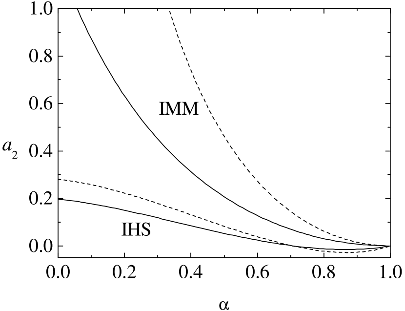
Figure 1: Plot of the fourth cumulant $a_{2}$ in the HCS for $d=3$ (solid lines) and $d=2$ (dashed lines).

3.2 White noise thermostat

Now we assume that the system is heated with the white noise thermostat represented by the operator (9) with $\gamma=\zeta$. Using again the scaled quantities (19), Eq. (1) becomes

$$\left[\partial_{\tau}-\frac{1-\alpha^{2}}{8d}\left(\frac{\partial}{\partial{\bf c}_{1}}\right)^{2}\right]\widetilde{f}({\bf c}_{1})=\widetilde{J}[\mathbf{c}_{1}|\widetilde{f}].$$ (26)

Taking moments we get

$$\partial_{\tau}\langle c^{s}\rangle-\frac{1-\alpha^{2}}{8d}s(s+d-2)\langle c^{s-2}\rangle=-\mu_{s}.$$ (27)

In particular, setting $s=4$,

$$\partial_{\tau}\langle c^{4}\rangle = -(1+\alpha)\frac{9+12d-\alpha(17+4d)+3\alpha^{2}(1-\alpha)}{8d(d+2)}$$ (28)

$$\times\left[\langle c^{4}\rangle-\frac{d(d+2)}{4}\frac{(3-\alpha)\left(4d+5-3\alpha(2+\alpha)\right)}{9+12d-\alpha(17+4d)+3\alpha^{2}(1-\alpha)}\right].$$

In the case of this thermostat, the moment $\langle c^{4}\rangle$ relaxes to a steady state value for any dimensionality $d$. The corresponding exact expression for the fourth cumulant is

$$a_{2}=\frac{6(1-\alpha)^{2}(1+\alpha)}{9+12d-\alpha(17+4d)+3\alpha^{2}(1-\alpha)}.$$ (29)

The cumulant $a_{2}$ for IHS in the nonequilibrium steady state driven by a white noise thermostat can be estimated to be [42]

$$a_{2}^{\text{IHS}}=\frac{16(1-\alpha)(1-2\alpha^{2})}{73+56d-3\alpha(35+8d)+30\alpha^{2}(1-\alpha)}.$$ (30)

Figure 2 shows that the differences between the values of $a_{2}$ for IMM and IHS are less dramatic than in the HCS. The behaviour observed in Fig 2 is in agreement with the high energy tails $\widetilde{f}(\mathbf{c})\sim\e^{-ac}$ for IMM [37] and $\widetilde{f}(\mathbf{c})\sim\e^{-ac^{3/2}}$ for IHS [42].

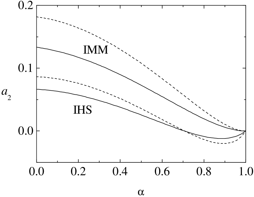
Figure 2: Plot of the fourth cumulant $a_{2}$ in the case of a system heated by a white noise thermostat for $d=3$ (solid lines) and $d=2$ (dashed lines).

It is interesting to remark that, according to Eqs. (24) and (29), $a_{2}\propto(1-\alpha)^{2}$ for IMM in the small inelasticity limit [29, 31], while $a_{2}\propto(1-\alpha)$ for IHS in the same limit [42].

4 Transport coefficients

The standard Chapman–Enskog method [1] can be generalized to inelastic collisions to obtain the dependence of the Navier–Stokes transport coefficients on the coefficient of restitution from the Boltzmann equation [43, 45, 46] and from the Enskog equation [44]. Here the method will be applied to the Boltzmann equation (1) for IMM.

In the Chapman–Enskog method a factor $\epsilon$ is assigned to every gradient operator and the distribution function is represented as a series in this formal “uniformity” parameter,

$$f=f^{(0)}+\epsilon f^{(1)}+\epsilon^{2}f^{(2)}+\cdots.$$ (31)

Use of this expansion in the definitions of the fluxes (13) and (14) and the cooling rate (15) gives the corresponding expansion for these quantities. Finally, use of these in the hydrodynamic equations (10)–(12) leads to an identification of the time derivatives of the fields as an expansion in the gradients,

$$\partial_{t}=\partial_{t}^{(0)}+\epsilon\partial_{t}^{(1)}+\epsilon^{2}\partial_{t}^{(2)}+\cdots.$$ (32)

In particular, the macroscopic balance equations to zeroth order become

$$\partial_{t}^{(0)}n=0,\quad\partial_{t}^{(0)}\mathbf{u}=\mathbf{0},\quad\partial_{t}^{(0)}T=-(\zeta-\gamma)T.$$ (33)

Here we have taken into account that in the Boltzmann equation (1) the effective collision frequency $\omega\propto nT^{1/2}$ is assumed to be a functional of $f$ only through the density $n$ and granular temperature $T$. Consequently, $\omega^{(0)}=\omega$, $\omega^{(1)}=\omega^{(2)}=\cdots=0$ and, using Eq. (16), $\zeta^{(0)}=\zeta$, $\zeta^{(1)}=\zeta^{(2)}=\cdots=0$. It must be noticed that, in the case of IHS, $\zeta^{(1)}=0$ and $\zeta^{(2)}$ is small [43].

To zeroth order in the gradients the kinetic equation (1) reads

$$\left(\frac{\zeta-\gamma}{2}\frac{\partial}{\partial\mathbf{V}}\cdot\mathbf{V}+\mathcal{F}\right)f^{(0)}(\mathbf{V})=J[\mathbf{V}|f^{(0)}],$$ (34)

where use has been made of the properties

$$\partial_{t}^{(0)}f^{(0)}(\mathbf{V})=-(\zeta-\gamma)T\frac{\partial}{\partial T}f^{(0)}(\mathbf{V})=\frac{\zeta-\gamma}{2}\frac{\partial}{\partial\mathbf{V}}\cdot\mathbf{V}f^{(0)}(\mathbf{V}),$$ (35)

the last equality following from the fact that the dependence of $f^{(0)}$ on the temperature is of the form $f^{(0)}(\mathbf{V})=nv_{0}^{-d}\widetilde{f}^{(0)}(\mathbf{V}/v_{0})$. In the undriven case ($\mathcal{F}=0$, $\gamma=0$), as well as in the case of the Gaussian thermostat (8) with $\gamma=\zeta$, Eq. (34) is equivalent to the homogeneous equation analyzed in Subsection 3.1. Therefore, $f^{(0)}(\mathbf{V})$ is given by the stationary solution to Eq. (20), except that $n\to n(\mathbf{r},t)$ and $T\to T(\mathbf{r},t)$ are local quantities and $\mathbf{v}\to\mathbf{V}=\mathbf{v}-\mathbf{u}(\mathbf{r},t)$. Analogously, in the case of the white noise thermostat (9) with $\gamma=\zeta$ Eq. (34) is equivalent to the homogeneous equation analyzed in Subsection 3.2.

Since $f^{(0)}$ is isotropic, it follows that

$$\mathsf{P}^{(0)}=p\mathsf{I},\quad\mathbf{q}^{(0)}=\mathbf{0},$$ (36)

where $p=nT$ is the hydrostatic pressure and $\mathsf{I}$ is the $d\times d$ unit tensor. Therefore, the macroscopic balance equations give

$$D_{t}^{(1)}n=-n\nabla\cdot\mathbf{u},\quad D_{t}^{(1)}\mathbf{u}=-\frac{\nabla p}{mn},\quad D_{t}^{(1)}T=-\frac{2T}{d}\nabla\cdot\mathbf{u},$$ (37)

where $D_{t}^{(1)}\equiv\partial_{t}^{(1)}+\mathbf{u}\cdot\nabla$. To first order in the gradients Eq. (1) leads to the following equation for $f^{(1)}$:

$$\left(\partial_{t}^{(0)}+\mathcal{L}+\mathcal{F}\right)f^{(1)}(\mathbf{V})=-\left(D_{t}^{(1)}+\mathbf{V}\cdot\nabla\right)f^{(0)}(\mathbf{V}),$$ (38)

where $\mathcal{L}$ is the linearized collision operator

$$\mathcal{L}f^{(1)}(\mathbf{V}_{1}) = -\frac{\omega}{n\Omega_{d}}\int\d\widehat{\bm{\sigma}}\int\d{\bf V}_{2}\left(\alpha^{-1}\widehat{b}^{-1}-1\right)$$ (39)

$$\times\left[f^{(0)}({\bf V}_{1})f^{(1)}({\bf V}_{2})+f^{(0)}({\bf V}_{2})f^{(1)}({\bf V}_{1})\right].$$

The collisional integrals of $\mathbf{V}\mathbf{V}$ and $V^{2}\mathbf{V}$ are evaluated in Appendix A. From the linearization of Eqs. (78) and (80) we have

$$m\int\d\mathbf{V}\,\mathbf{V}\mathbf{V}\mathcal{L}f^{(1)}(\mathbf{V})=\nu\mathsf{P}^{(1)},$$ (40)

$$\frac{m}{2}\int\d\mathbf{V}\,V^{2}\mathbf{V}\mathcal{L}f^{(1)}(\mathbf{V})=\left(\frac{d-1}{d}\nu+\frac{d+2}{2d}\zeta\right)\mathbf{q}^{(1)},$$ (41)

where the collision frequency $\nu$ is

$$\nu\equiv\omega\frac{(1+\alpha)(d+1-\alpha)}{d(d+2)}.$$ (42)

Using (37), the right-hand side of Eq. (38) can be written as

$$-\left(D_{t}^{(1)}+\mathbf{V}\cdot\nabla\right)f^{(0)}(\mathbf{V})={\bf A}(\mathbf{V})\cdot\nabla\ln T+{\bf B}(\mathbf{V})\cdot\nabla\ln n+\mathsf{C}(\mathbf{V}):\nabla\mathbf{u},$$ (43)

where

$${\bf A}\equiv\frac{\bf V}{2}\frac{\partial}{\partial{\bf V}}\cdot\left({\bf V}f^{(0)}\right)-\frac{T}{m}\frac{\partial}{\partial{\bf V}}f^{(0)},$$ (44)

$${\bf B}\equiv-{\bf V}f^{(0)}-\frac{T}{m}\frac{\partial}{\partial{\bf V}}f^{(0)},$$ (45)

$$C_{ij}\equiv\frac{\partial}{\partial V_{i}}\left(V_{j}f^{(0)}\right)-\frac{1}{d}\delta_{ij}\frac{\partial}{\partial{\bf V}}\cdot\left({\bf V}f^{(0)}\right).$$ (46)

Now we multiply both sides of Eq. (38) by $mV_{i}V_{j}$ and integrate over ${\bf V}$. The result is

$$(\partial_{t}^{(0)}+\nu)P_{ij}^{(1)}+\Pi_{ij}^{(1)}=-p\Delta_{ijkl}\nabla_{k}u_{l},$$ (47)

where

$$\Pi_{ij}^{(1)}\equiv m\int\d\mathbf{V}\,V_{i}V_{j}\mathcal{F}f^{(1)}(\mathbf{V})$$ (48)

and

$$\Delta_{ijkl}\equiv\delta_{ik}\delta_{jl}+\delta_{il}\delta_{jk}-\frac{2}{d}\delta_{ij}\delta_{kl}.$$ (49)

Of course, $\Pi_{ij}^{(1)}=0$ in the undriven case. For driven systems,

$$\Pi_{ij}^{(1)}=\left\{\begin{array}[]{ll}-\zeta P_{ij}^{(1)}&\text{(Gaussian thermostat)},\\ 0&\text{(white noise thermostat)}.\end{array}\right.$$ (50)

The solution to Eq. (47) has the form

$$P_{ij}^{(1)}=-\eta\Delta_{ijkl}\nabla_{k}u_{l},$$ (51)

where $\eta$ is the shear viscosity. By dimensional analysis, $\eta\propto T^{1/2}$. Therefore,

$$\partial_{t}^{(0)}\mathsf{P}^{(1)}=-\frac{\zeta-\gamma}{2}\mathsf{P}^{(1)}.$$ (52)

Consequently, Eq. (47) yields

$$\eta=p\left\{\begin{array}[]{ll}\left({\nu-\frac{1}{2}\zeta}\right)^{-1}&\text{(undriven system)},\\ \left({\nu-\zeta}\right)^{-1}&\text{(Gaussian thermostat)},\\ {\nu}^{-1}&\text{(white noise thermostat)}.\end{array}\right.$$ (53)

Except for a possible $\alpha$–dependence of $\nu$ [cf. Eq. (68) below], the result $\eta=p/\nu$ in the case of the white noise thermostat is the same as for elastic particles. This allows us to interpret $\nu^{-1}$ as the effective mean free time associated with momentum transport. This formal equivalence between the shear viscosity of a fluid of elastic particles and that of a granular fluid driven by a white noise forcing is due to the fact that the latter forcing, while compensating for the inelastic cooling, does not contribute to the rate of change of the stress tensor. The Gaussian thermostat, on the other hand, yields a term $\zeta\mathsf{P}^{(1)}$ and therefore tends to produce a temporal increase in the magnitude of the stress tensor, thus partially cancelling the dissipative term $-\nu\mathsf{P}^{(1)}$. As a consequence, the steady-state shear viscosity is enhanced, $\eta=p/(\nu-\zeta)$. Finally, in the absence of any external driving, the state is unsteady and so the inelastic cooling is responsible for a smaller enhancement of the shear viscosity, $\eta=p/(\nu-\zeta/2)$. It is worth noting that a structure similar to that of Eq. (53) is also present in the cases of the Boltzmann equation for IHS [cf. Eq. (89)] and the BGK-like kinetic model [cf. Eq. (98)].

Let us consider next the heat flux. Multiplying both sides of Eq. (38) by $\frac{1}{2}mV^{2}\mathbf{V}$ and integrating over ${\bf V}$ we get

$$\left(\partial_{t}^{(0)}+\nu^{\prime}\right){\bf q}^{(1)}+\mathbf{Q}^{(1)}=-\frac{d+2}{2}(1+2a_{2})\frac{p}{m}\nabla T-\frac{d+2}{2}a_{2}\frac{T^{2}}{m}\nabla n,$$ (54)

where

$$\nu^{\prime}\equiv\frac{d-1}{d}\nu+\frac{d+2}{2d}\zeta=\frac{4(d-1)+(8+d)(1-\alpha)}{4d+4(1-\alpha)}\nu$$ (55)

is an effective collision frequency associated with the thermal conductivity and

$$\mathbf{Q}^{(1)}\equiv\frac{m}{2}\int\d\mathbf{V}\,V^{2}\mathbf{V}\mathcal{F}f^{(1)}(\mathbf{V}).$$ (56)

In the undriven case, $\mathbf{Q}^{(1)}=\mathbf{0}$. For the types of driving we are considering,

$$\mathbf{Q}^{(1)}=\left\{\begin{array}[]{ll}-\frac{3}{2}\zeta\mathbf{q}^{(1)}&\text{(Gaussian thermostat)},\\ \mathbf{0}&\text{(white noise thermostat)}.\end{array}\right.$$ (57)

The heat flux has the structure

$${\bf q}^{(1)}=-\lambda\nabla T-\mu\nabla n,$$ (58)

where $\lambda$ is the thermal conductivity and $\mu$ is a transport coefficient with no counterpart for elastic particles [43]. Dimensional analysis shows that $\lambda\propto T^{1/2}$ and $\mu\propto T^{3/2}$. Consequently,

$$\partial_{t}^{(0)}{\bf q}^{(1)} = \frac{1}{2}(\zeta-\gamma)\lambda\nabla T+\frac{3}{2}(\zeta-\gamma)\mu\nabla n+\lambda\nabla(\zeta-\gamma)T$$ (59)

$$= (\zeta-\gamma)\left[2\lambda\nabla T+\left(\frac{3}{2}\mu+\lambda\frac{T}{n}\right)\nabla n\right],$$

where in the last step we have taken into account that $\zeta,\gamma\propto nT^{1/2}$. Inserting this equation into Eq. (54), we can identify the transport coefficients as

$$\lambda=\frac{p}{m}\frac{d+2}{2}\left(1+2a_{2}\right)\left\{\begin{array}[]{ll}\left({\nu^{\prime}-2\zeta}\right)^{-1}&\text{(undriven system)},\\ \left({\nu^{\prime}-\frac{3}{2}\zeta}\right)^{-1}&\text{(Gaussian thermostat)},\\ {\nu^{\prime}}^{-1}&\text{(white noise thermostat)},\end{array}\right.$$ (60)

$$\mu=\frac{T}{n}\frac{\lambda}{1+2a_{2}}\left\{\begin{array}[]{ll}\left({\zeta+a_{2}\nu^{\prime}}\right)\left({\nu^{\prime}-\frac{3}{2}\zeta}\right)^{-1}&\text{(undriven system)},\\ a_{2}&\text{(Gaussian thermostat)},\\ a_{2}&\text{(white noise thermostat)}.\end{array}\right.$$ (61)

In Eqs. (60) and (61), the cumulant $a_{2}$ is given by Eqs. (24) (undriven system and Gaussian thermostat) and (29) (white noise thermostat).

Using Eqs. (16) and (42), it can be seen that the thermal conductivity in the undriven case is $\lambda\propto(\alpha-\alpha_{0})^{-1}$, where $\alpha_{0}=(4-d)/3d$. This implies that the coefficients $\lambda$ and $\mu$ exhibit an unphysical behaviour for $d=2$ and $d=3$ since they diverge at $\alpha=\alpha_{0}$ and become negative for $0\leq\alpha<\alpha_{0}$. This singular behaviour is absent in the shear viscosity $\eta$ or in $\lambda$ and $\mu$ for thermostatted states because $\nu>\zeta$ for all $\alpha$ and $d$.

In order to have the full $\alpha$–dependence of the transport coefficients we need to fix the free parameter $\omega(\alpha)$. This point will be addressed in Section 5. On the other hand, the ratios between transport coefficients are independent of the criterion to choose $\omega(\alpha)$. Let us define a generalized Prandtl number (for $d\neq 1$)

$$R_{\eta}(\alpha)=\frac{\eta(\alpha)/\eta_{0}}{\lambda(\alpha)/\lambda_{0}},$$ (62)

where $\eta_{0}$ and $\lambda_{0}$ are the shear viscosity and thermal conductivity, respectively, in the elastic limit ($\alpha=1$). From Eqs. (53) and (60) we have

$$R_{\eta}(\alpha)=\frac{1}{1+2a_{2}}\left\{\begin{array}[]{ll}\frac{d(d-4+3d\alpha)}{(d-1)[3d+2+(d-2)\alpha]}&\text{(undriven system)},\\ 1&\text{(Gaussian thermostat)},\\ \frac{d[5d+4-(d+8)\alpha]}{4(d-1)(d+1-\alpha)}&\text{(white noise thermostat)}.\end{array}\right.$$ (63)

Analogously, we can define the ratio

$$R_{\mu}(\alpha)=\frac{n\mu(\alpha)}{T\lambda(\alpha)}.$$ (64)

Thus,

$$R_{\mu}(\alpha)=\frac{1}{1+2a_{2}}\left\{\begin{array}[]{ll}\frac{d+2}{d-1}\frac{1-\alpha}{1+\alpha}+\frac{5d+4-(d+8)\alpha}{2(d-1)(1+\alpha)}a_{2}&\text{(undriven system)},\\ a_{2}&\text{(Gaussian thermostat)},\\ a_{2}&\text{(white noise thermostat)}.\end{array}\right.$$ (65)

5 Comparison with the transport coefficients of inelastic hard spheres

The transport coefficients of IHS described by the Boltzmann equation have been derived both for undriven [43, 44, 45] and thermostatted [46] systems in the first Sonine approximation. For the sake of completeness, the expressions of the transport coefficients of IHS are listed in Appendix B.

Figures 3 and 4 compare the ratios $R_{\eta}(\alpha)$, Eq. (62), and $R_{\mu}(\alpha)$, Eq. (64), for IMM and IHS in the three-dimensional case. It is observed that, in general, the results for IMM describe qualitatively the $\alpha$–dependence of $R_{\eta}$ and $R_{\mu}$ for IHS. Thus, as the inelasticity increases, the generalized Prandtl number $R_{\eta}$ decreases in the absence of external forcing and increases in the case of the white noise thermostat. With the Gaussian thermostat, however, the discrepancies are important: $R_{\eta}$ increases with the inelasticity for IHS and decreases for IMM. As for the ratio $R_{\mu}$, which measures the new transport coefficient $\mu$ relative to the thermal conductivity, it rapidly increases in the unforced case, while it is very small in the driven cases. At a quantitative level, the IMM results exhibit important deviations from the IHS ones, especially in the undriven case, where $R_{\eta}$ for IMM becomes negative when $\alpha<\alpha_{0}=\frac{1}{9}$ and $R_{\mu}$ grows too rapidly. The situation in which the IMM ratios are the closest to the IHS ones corresponds to the system heated by a white noise thermostat.

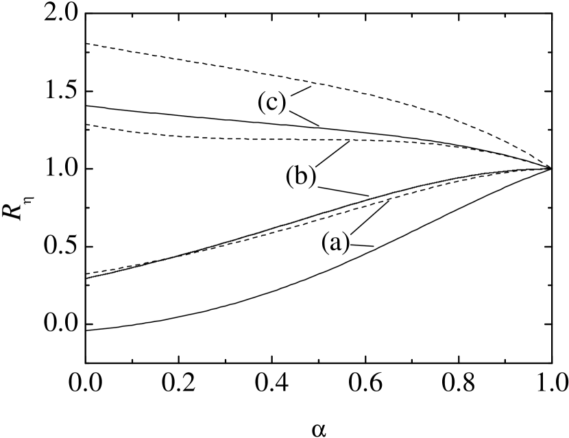
Figure 3: Plot of the generalized Prandtl number $R_{\eta}(\alpha)$ from the Boltzmann equation for three-dimensional IMM (solid lines) and IHS (dashed lines) for (a) undriven systems, (b) Gaussian thermostat and (c) white noise thermostat. The curves corresponding to IMM in case (b) and to IHS in case (a) are very close each other by accident.

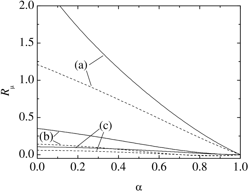
Figure 4: Plot of the ratio $R_{\mu}(\alpha)$ from the Boltzmann equation for three-dimensional IMM (solid lines) and IHS (dashed lines) for (a) undriven systems, (b) Gaussian thermostat and (c) white noise thermostat.

Of course, the most interesting comparison refers to the three transport coefficients themselves, rather than to their ratios. In order to have explicit expressions for the transport coefficients of IMM, we now need a criterion to fix the free parameter $\omega(\alpha)$. The most natural choice to optimize the agreement with the IHS results is to guarantee that the cooling rate for IMM, Eq. (16), be the same as that for IHS. Strictly speaking, the cooling rate for IHS depends in general on the details of the nonequilibrium velocity distribution function, while the effective collision frequency $\omega(\alpha)$ in Eq. (1) is assumed to depend on $f$ only through the density and the granular temperature. Otherwise, the complete knowledge of $\omega$ would require to solve first the Boltzmann equation for IHS and then evaluate the cooling rate associated with such a solution, what is impractical. Therefore, here I take for $\zeta$ the cooling rate of IHS at local equilibrium, namely,

$$\zeta=\nu_{0}\frac{d+2}{4d}(1-\alpha^{2}),$$ (66)

where $\nu_{0}$ is given by Eq. (92). Making use of Eqs. (16) and (42), this is equivalent to

$$\omega=\nu_{0}\frac{d+2}{2},$$ (67)

$$\nu=\nu_{0}\frac{(1+\alpha)(d+1-\alpha)}{2d}.$$ (68)

With this choice, Eqs. (53), (60) and (61) become, respectively,

$$\eta=\eta_{0}\frac{2d}{1+\alpha}\left\{\begin{array}[]{ll}4\left[3d+2+(d-2)\alpha\right]^{-1}&\text{(undriven system)},\\ \frac{2}{d}\left(1+\alpha\right)^{-1}&\text{(Gaussian thermostat)},\\ \left(d+1-\alpha\right)^{-1}&\text{(white noise thermostat)},\end{array}\right.$$ (69)

$$\lambda=\lambda_{0}\frac{8(d-1)}{1+\alpha}(1+2a_{2})\left\{\begin{array}[]{ll}\left(d-4+3d\alpha\right)^{-1}&\text{(undriven system)},\\ \frac{1}{2(d-1)}\left(1+\alpha\right)^{-1}&\text{(Gaussian thermostat)},\\ \left[5d+4-(d+8)\alpha\right]^{-1}&\text{(white noise thermostat)},\end{array}\right.$$ (70)

$$\mu=\frac{T}{n}\lambda_{0}\frac{4}{(1+\alpha)^{2}}\left\{\begin{array}[]{ll}\frac{2(d+2)(1-\alpha)}{d-4+3d\alpha}+\frac{5d+4-(d+8)\alpha}{d-4+3d\alpha}a_{2}&\text{(undriven system)},\\ a_{2}&\text{(Gaussian thermostat)},\\ \frac{2(d-1)(1+\alpha)}{5d+4-(d+8)\alpha}a_{2}&\text{(white noise thermostat)},\end{array}\right.$$ (71)

Figures 5–7 compare the three transport coefficients of IMM with those of IHS. For completeness, also the coefficients derived from a simple BGK-like model (see Appendix C) are included. Again, the qualitative behaviour of IHS is generally captured by the IMM. We observe that the shear viscosity increases with the inelasticity, the increase being more (less) important when the system is heated with a Gaussian (white noise) thermostat. The thermal conductivity increases with the inelasticity in a significant way in the undriven case, increases more moderately in the case of the Gaussian thermostat, and is almost constant in the case of the white noise thermostat. As for the transport coefficient $\mu$, it remains small in the thermostatted states, while it rapidly increases in the undriven state. All these trends are, however, strongly exaggerated by the IMM in the undriven case (where $\lambda$ and $\mu$ diverge at $\alpha=\alpha_{0}=\frac{1}{9}$) and, to a lesser extent, in the Gaussian thermostat case, especially for the coefficient $\mu$. On the other hand, the simple BGK-like model [25] summarized in Appendix C describes fairly well the $\alpha$–dependence of the three transport coefficients, being closer to the IHS results than the IMM predictions.

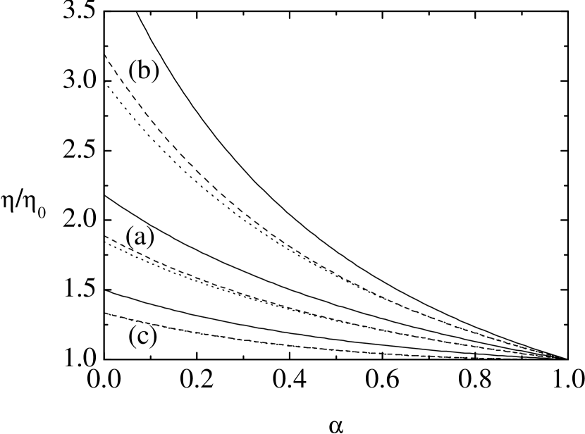
Figure 5: Plot of the reduced shear viscosity $\eta/\eta_{0}$ from the Boltzmann equation for three-dimensional IMM (solid lines) and IHS (dashed lines), as well as from the BGK-like model of IHS (dotted lines), for (a) undriven systems, (b) Gaussian thermostat and (c) white noise thermostat. The dashed and dotted lines are practically indistinguishable in case (c).

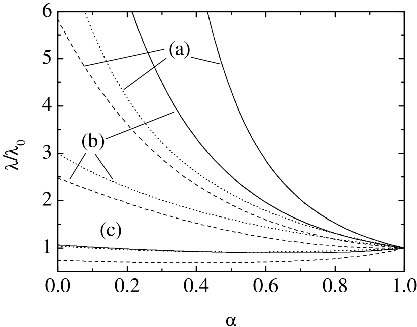
Figure 6: Plot of the reduced thermal conductivity $\lambda/\lambda_{0}$ from the Boltzmann equation for three-dimensional IMM (solid lines) and IHS (dashed lines), as well as from the BGK-like model of IHS (dotted lines), for (a) undriven systems, (b) Gaussian thermostat and (c) white noise thermostat. Note that the curves corresponding to IMM and the BGK-like model in case (c) are hardly distinguishable.

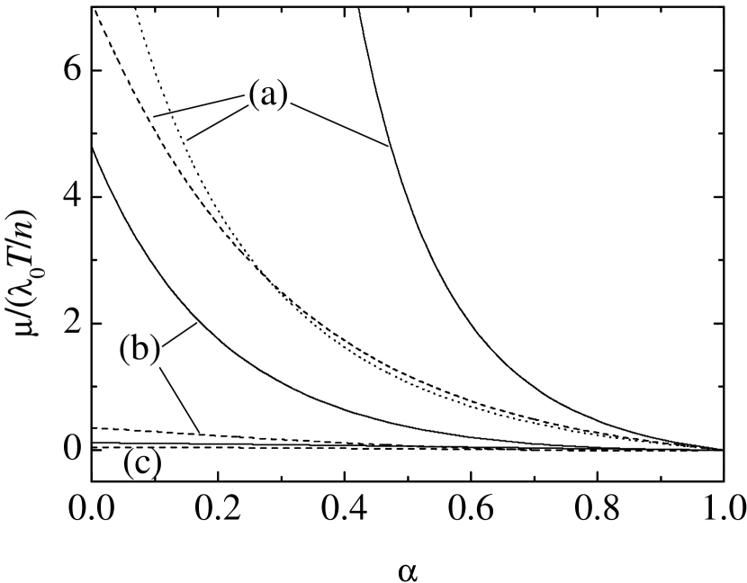
Figure 7: Plot of the reduced transport coefficient $\mu/(T\lambda_{0}/n)$ from the Boltzmann equation for three-dimensional IMM (solid lines) and IHS (dashed lines), as well as from the BGK-like model of IHS (dotted line), for (a) undriven systems, (b) Gaussian thermostat and (c) white noise thermostat. Note that the BGK-like model predicts $\mu=0$ in cases (b) and (c).

6 Concluding remarks

In the Boltzmann equation for inelastic Maxwell models (IMM), the collision rate of the underlying system of inelastic hard spheres (IHS) is replaced by an effective collision rate independent of the relative velocity of the colliding particles. Based on the experience in the case of elastic particles, one might reasonably think that this model, while making the collision operator mathematically more tractable, is able to capture the most important properties of IHS, at least those relatively insensitive to the domain of velocities much larger than the thermal velocity. In particular, one might expect the three transport coefficients (shear viscosity, thermal conductivity and the coefficient associated with the contribution of a density gradient to the heat flux) of IMM to possess a dependence on the coefficient of restitution similar to that of the transport coefficients of IHS. The results derived in this paper show, however, that this expectation does not hold true, except at a mild qualitative level, even if the IMM is made to reproduce the cooling rate of IHS. On the other hand, a model kinetic equation based on the well-known BGK model for elastic collisions presents a surprisingly good agreement with IHS, once the limitation of the BGK model to reproduce the correct Prandtl number of elastic particles is conveniently accounted for. A partial explanation of this paradox may lie in the fact that in the IMM a rough approximation (collision rate independent of the relative velocity) coexists with the remaining complexity of the detailed collision process. As a result, only a free parameter (essentially the cooling rate) is available to make contact with IHS. In the BGK-like model, however, the cooling rate and its dominant effect on the velocity distribution function is explicitly taken out; what remains of the Boltzmann collision operator is modelled by a conventional relaxation-time term reflecting the effects of collisions not directly associated with the energy dissipation. As a consequence, in addition to the cooling rate, the BGK-like model incorporates an effective (velocity-independent) collision frequency that increases the flexibility of the model in spite of its simplicity.

In conclusion, the IMM is interesting as a mathematical toy model to explore how a small degree of collisional inelasticity may have a strong influence on the physical properties of the system. For instance, the velocity moments in homogeneous states can be evaluated only approximately in IHS [42], while they can be exactly obtained in IMM [29]; the high energy tail is another example where rather detailed information can be obtained from the Boltzmann equation for IMM [19, 20, 33, 35, 37]. On the other hand, if one is looking for a “shortcut” to know some of the properties of IHS, the use of the IMM requires a great deal of caution. First, the solution of the Boltzmann equation for IMM may still be a formidable task, except in some special cases. Second, the results derived from the IMM may not be sufficiently representative of the behaviour of IHS, as exemplified here in the case of the transport coefficients. From that point of view, it seems preferable to make use of the BGK-like model proposed in Ref. [25]. For instance, this model has an exact solution for the nonlinear planar Couette flow (with combined momentum and energy transport) that compares quite well with DSMC data for IHS [28]; for this flow, however, the Boltzmann equation for IMM cannot be solved in a closed form, even in the elastic limit [16].

Appendix A Collisional moments

Let us consider the general collisional integral of the form

$$I[F]\equiv\int\d\mathbf{v}\,F(\mathbf{v})J[\mathbf{v}|f].$$ (72)

By following standard steps, $I[F]$ can be written as

$$I[F]=\frac{\omega}{2n\Omega_{d}}\int\d{\bf v}_{1}\int\d{\bf v}_{2}\int\d\widehat{\bm{\sigma}}f({\bf v}_{1})f({\bf v}_{2})\left(\widehat{b}-1\right)\left[F(\mathbf{v}_{1})+F(\mathbf{v}_{2})\right].$$ (73)

Now we particularize to $F(\mathbf{v})=\mathbf{V}\mathbf{V}$. From the collision rule (2) it follows that

$$\left(\widehat{b}-1\right)({\bf V}_{1}{\bf V}_{1}+{\bf V}_{2}{\bf V}_{2})=\frac{1+\alpha}{2}({\bf g}\cdot\widehat{\bm{\sigma}})\left[(1+\alpha)({\bf g}\cdot\widehat{\bm{\sigma}})\widehat{\bm{\sigma}}\widehat{\bm{\sigma}}-{\bf g}\widehat{\bm{\sigma}}-\widehat{\bm{\sigma}}{\bf g}\right].$$ (74)

To perform the angular integrations we need the results

$$\int\d\widehat{\bm{\sigma}}\,({\bf g}\cdot\widehat{\bm{\sigma}})^{2}\widehat{\bm{\sigma}}\widehat{\bm{\sigma}}=B_{2}{\bf g}{\bf g}+\frac{B_{1}-B_{2}}{d-1}\left(g^{2}{\sf I}-{\bf g}{\bf g}\right),$$ (75)

$$\int\d\widehat{\bm{\sigma}}\,({\bf g}\cdot\widehat{\bm{\sigma}})\widehat{\bm{\sigma}}=B_{1}{\bf g},$$ (76)

where [20]

$$B_{n}\equiv\int\d\widehat{\bm{\sigma}}\,(\widehat{\bf g}\cdot\widehat{\bm{\sigma}})^{2n}=\Omega_{d}\pi^{-1/2}\frac{\Gamma(d/2)\Gamma(n+1/2)}{\Gamma(n+d/2)}$$ (77)

and $\mathsf{I}$ is the $d\times d$ unit tensor. Therefore,

$$I[\mathbf{V}\mathbf{V}] = -\omega\frac{1+\alpha}{4nd}\int\d{\bf v}_{1}\int\d{\bf v}_{2}\,f({\bf v}_{1})f({\bf v}_{2})\left[\frac{1-\alpha}{d}g^{2}{\sf I}\right.$$ (78)

$$\left.+2\frac{d+1-\alpha}{d+2}\left({\bf g}{\bf g}-\frac{1}{d}g^{2}{\sf I}\right)\right]$$

$$= -\omega\frac{1+\alpha}{2md}\left[(1-\alpha)p{\sf I}+2\frac{d+1-\alpha}{d+2}\left({\sf P}-p{\sf I}\right)\right].$$

The cooling rate is $\zeta=-(m/dnT)I[V^{2}]$, so taking the trace of Eq. (78) we get Eq. (16).

Next we particularize to $F(\mathbf{v})=V^{2}\mathbf{V}$. The collision rule gives

$$\left(\widehat{b}-1\right)(V_{1}^{2}{\bf V}_{1}+V_{2}^{2}{\bf V}_{2}) = \left(\frac{1+\alpha}{2}\right)^{2}({\bf g}\cdot\widehat{\bm{\sigma}})^{2}({\bf V}_{1}+{\bf V}_{2})\cdot({\sf I}+2\widehat{\bm{\sigma}}\widehat{\bm{\sigma}})$$ (79)

$$-\frac{1+\alpha}{2}\left({\bf g}\cdot\widehat{\bm{\sigma}})(V_{1}^{2}{\sf I}+2{\bf V}_{1}{\bf V}_{1}\right.$$

$$\left.-V_{2}^{2}{\sf I}-2{\bf V}_{2}{\bf V}_{2}\right)\cdot\widehat{\bm{\sigma}}.$$

After performing the angular integrations one has

$$I[V^{2}\mathbf{V}] = \frac{\omega(1+\alpha)}{4nd}\int\d{\bf v}_{1}\int\d{\bf v}_{2}\,f({\bf v}_{1})f({\bf v}_{2})$$ (80)

$$\times\left\{\frac{1+\alpha}{2(d+2)}({\bf V}_{1}+{\bf V}_{2})\cdot[(d+4)g^{2}{\sf I}+4{\bf g}{\bf g}]\right.$$

$$\left.-{\bf g}\cdot(V_{1}^{2}{\sf I}+2{\bf V}_{1}{\bf V}_{1}-V_{2}^{2}{\sf I}-2{\bf V}_{2}{\bf V}_{2})\right\}$$

$$= -\frac{2\omega(1+\alpha)(d-1)}{md(d+2)}\left(1+\frac{d+8}{d-1}\frac{1-\alpha}{4}\right){\bf q}.$$

Finally, let us evaluate the collisional moment $\mu_{4}$, where $\mu_{s}$ is defined by the last identity in Eq. (21), i.e.,

$$\mu_{4}=-\frac{1}{2\Omega_{d}}\int\d\widehat{\bm{\sigma}}\int\d{\bf c}_{1}\int\d{\bf c}_{2}\,\widetilde{f}({\bf c}_{1})\widetilde{f}({\bf c}_{2})\left(\widehat{b}-1\right)(c_{1}^{4}+c_{2}^{4}).$$ (81)

From the collision rule one gets [42]

$$\left(\widehat{b}-1\right)(c_{1}^{4}+c_{2}^{4}) = 2(1+\alpha)^{2}({\bf g}\cdot\widehat{\bm{\sigma}})^{2}({\bf G}\cdot\widehat{\bm{\sigma}})^{2}+\frac{1}{8}(1-\alpha^{2})^{2}({\bf g}\cdot\widehat{\bm{\sigma}})^{4}$$ (82)

$$-(1-\alpha^{2})({\bf g}\cdot\widehat{\bm{\sigma}})^{2}\left(G^{2}+\frac{1}{4}g^{2}\right)$$

$$-4(1+\alpha)({\bf g}\cdot\widehat{\bm{\sigma}})({\bf G}\cdot\widehat{\bm{\sigma}})({\bf g}\cdot{\bf G}),$$

where $\mathbf{G}\equiv\frac{1}{2}(\mathbf{c}_{1}+\mathbf{c}_{2})$. Equations (75) and (76) give

$$\int\d\widehat{\bm{\sigma}}\,({\bf g}\cdot\widehat{\bm{\sigma}})^{2}({\bf G}\cdot\widehat{\bm{\sigma}})^{2}=\frac{\Omega_{d}}{d(d+2)}\left[2({\bf g}\cdot{\bf G})^{2}+g^{2}G^{2}\right],$$ (83)

$$\int\d\widehat{\bm{\sigma}}\,({\bf g}\cdot\widehat{\bm{\sigma}})({\bf G}\cdot\widehat{\bm{\sigma}})=\frac{\Omega_{d}}{d}({\bf g}\cdot{\bf G}).$$ (84)

Therefore,

$$\mu_{4} = -\frac{1+\alpha}{2d}\int d{\bf c}_{1}\int d{\bf c}_{2}\,\widetilde{f}({\bf c}_{1})\widetilde{f}({\bf c}_{2})\left\{\frac{2(1+\alpha)}{d+2}\left[2({\bf g}\cdot{\bf G})^{2}+g^{2}G^{2}\right]\right.$$ (85)

$$\left.+\frac{3(1-\alpha)^{2}(1+\alpha)}{8(d+2)}g^{4}-(1-\alpha)g^{2}\left(G^{2}+\frac{1}{4}g^{2}\right)-4({\bf g}\cdot{\bf G})^{2}\right\}$$

Finally, by taking into account that

$$({\bf g}\cdot{\bf G})^{2}=\frac{1}{4}(c_{1}^{4}+c_{2}^{4}-2c_{1}^{2}c_{2}^{2}),$$ (86)

$$g^{2}G^{2}=\frac{1}{4}[c_{1}^{4}+c_{2}^{4}+2c_{1}^{2}c_{2}^{2}-4({\bf c}_{1}\cdot{\bf c}_{2})^{2}],$$ (87)

$$g^{4}=c_{1}^{4}+c_{2}^{4}+2c_{1}^{2}c_{2}^{2}+4({\bf c}_{1}\cdot{\bf c}_{2})^{2}-4(c_{1}^{2}+c_{2}^{2})({\bf c}_{1}\cdot{\bf c}_{2}),$$ (88)

we get Eq. (22).

Appendix B Transport coefficients of inelastic hard spheres

The derivation of the Navier–Stokes transport coefficients for IHS can be found in Refs. [43, 44, 45, 46]. In the first Sonine approximation, the results are

$$\eta=\frac{p}{\nu_{0}}\left\{\begin{array}[]{ll}\left({\nu_{\eta}^{*}-\frac{1}{2}\zeta^{*}}\right)^{-1}&\text{(undriven system)},\\ \left({\nu_{\eta}^{*}-\zeta^{*}}\right)^{-1}&\text{(Gaussian thermostat)},\\ {\nu_{\eta}^{*}}^{-1}&\text{(white noise thermostat)},\end{array}\right.$$ (89)

$$\lambda=\frac{p}{m\nu_{0}}\frac{d+2}{2}\left(1+2a_{2}^{\text{IHS}}\right)\left\{\begin{array}[]{ll}\left({\nu_{\lambda}^{*}-2\zeta^{*}}\right)^{-1}&\text{(undriven system)},\\ \left({\nu_{\lambda}^{*}-\frac{3}{2}\zeta^{*}}\right)^{-1}&\text{(Gaussian thermostat)},\\ {\nu_{\lambda}^{*}}^{-1}&\text{(white noise thermostat)},\end{array}\right.$$ (90)

$$\mu=\frac{T}{n}\frac{\lambda}{1+2a_{2}^{\text{IHS}}}\left\{\begin{array}[]{ll}\left({\zeta^{*}+a_{2}^{\text{IHS}}\nu_{\lambda}^{*}}\right)\left({\nu_{\lambda}^{*}-\frac{3}{2}\zeta^{*}}\right)^{-1}&\text{(undriven system)},\\ a_{2}^{\text{IHS}}&\text{(Gaussian thermostat)},\\ a_{2}^{\text{IHS}}&\text{(white noise thermostat)}.\end{array}\right.$$ (91)

In these equations [45],

$$\nu_{0}=n\sigma^{d-1}(T/m)^{1/2}\frac{4\Omega_{d}}{\pi^{1/2}(d+2)},$$ (92)

$$\zeta^{*}=\frac{d+2}{4d}(1-\alpha^{2})\left(1+\frac{3}{16}a_{2}^{\text{IHS}}\right),$$ (93)

$$\nu_{\eta}^{*}=\frac{3}{4d}\left(1-\alpha+\frac{2}{3}d\right)(1+\alpha)\left(1-\frac{1}{32}a_{2}^{\text{IHS}}\right),$$ (94)

$$\nu_{\lambda}^{*}=\frac{1+\alpha}{d}\left[\frac{d-1}{2}+\frac{3}{16}(d+8)(1-\alpha)+\frac{4+5d-3(4-d)\alpha}{512}a_{2}^{\text{IHS}}\right].$$ (95)

The expressions for $a_{2}^{\text{IHS}}$ are given by Eq. (25) for the undriven case and for the Gaussian thermostat and by Eq. (30) for the white noise thermostat.

Appendix C BGK-like model

In its simplest version, the BGK-like model proposed in Ref. [25] reads

$$(\partial_{t}+{\bf v}\cdot\nabla+\mathcal{F})f({\bf r},{\bf v};t) = -\left(\nu_{\text{BGK}}-\zeta\right)\left[f({\bf r},{\bf v};t)-f_{0}({\bf r},{\bf v};t)\right]$$ (96)

$$+\frac{1}{2}\zeta\frac{\partial}{\partial{\bf v}}\cdot\mathbf{V}f(\mathbf{r},\mathbf{v};t),$$

where $\nu_{\text{BGK}}\propto nT^{1/2}$ is an effective collision frequency and $f_{0}$ is the local equilibrium distribution function. The BGK-like model (96) can be interpreted as indicating that a system of inelastic hard spheres behaves essentially as a system of elastic hard spheres with a modified $\alpha$-dependent rate of collisions and subjected to the action of a “friction” force $-\frac{1}{2}m\zeta\mathbf{V}$, which accounts for the energy dissipation in an effective way. Applying the Chapman–Enskog method to Eq. (96) one obtains Eq. (38) with $f^{(0)}=f_{0}$ and the replacement

$$\mathcal{L}f^{(1)}\to\left(\nu_{\text{BGK}}-\zeta-\frac{1}{2}\zeta\frac{\partial}{\partial{\bf V}}\cdot\mathbf{V}\right)f^{(1)}.$$ (97)

It is then straightforward to get the transport coefficients as

$$\eta=p\left\{\begin{array}[]{ll}\left({\nu_{\text{BGK}}-\frac{1}{2}\zeta}\right)^{-1}&\text{(undriven system)},\\ \left({\nu_{\text{BGK}}-\zeta}\right)^{-1}&\text{(Gaussian thermostat)},\\ {\nu_{\text{BGK}}}^{-1}&\text{(white noise thermostat)},\end{array}\right.$$ (98)

$$\lambda=\frac{p}{m}\frac{d+2}{2}\left\{\begin{array}[]{ll}\left(\nu_{\text{BGK}}-\frac{3}{2}\zeta\right)^{-1}&\text{(undriven system)},\\ \left(\nu_{\text{BGK}}-\zeta\right)^{-1}&\text{(Gaussian thermostat)},\\ \left(\nu_{\text{BGK}}+\frac{1}{2}\zeta\right)^{-1}&\text{(white noise thermostat)},\end{array}\right.$$ (99)

$$\mu=\frac{T}{n}\lambda\left\{\begin{array}[]{ll}{\zeta}\left({\nu_{\text{BGK}}-\zeta}\right)^{-1}&\text{(undriven system)},\\ 0&\text{(Gaussian thermostat)},\\ 0&\text{(white noise thermostat)}.\end{array}\right.$$ (100)

Strictly speaking, the cooling rate $\zeta$ is a functional of the velocity distribution function through Eq. (15). In the spirit of the kinetic model (96), the exact cooling rate $\zeta$ is approximated by its local equilibrium expression

$$\zeta(\alpha)\to\nu_{0}\frac{d+2}{4d}(1-\alpha^{2}),$$ (101)

where $\nu_{0}\propto nT^{1/2}$ is a collision frequency (independent of $\alpha$) defined by Eq. (92). It remains to fix the $\alpha$–dependence of $\nu_{\text{BGK}}$. Comparison between Eqs. (89) and (98) suggests the identification $\nu_{\text{BGK}}\to\nu_{0}\nu_{\eta}^{*}$ as the simplest choice. Thus,

$$\nu_{\text{BGK}}=\nu_{0}\frac{3}{4d}\left(1-\alpha+\frac{2}{3}d\right)(1+\alpha),$$ (102)

where we have set $a_{2}^{\text{IHS}}\to 0$, in consistency with the local equilibrium approximation (101) for the cooling rate. Inserting Eqs. (101) and (102) into Eqs. (98)–(100), one gets

$$\eta(\alpha)=\eta_{0}\frac{4d}{1+\alpha}\left\{\begin{array}[]{ll}2\left[4+3d-(4-d)\alpha\right]^{-1}&\text{(undriven system)},\\ \left[1+d+(d-1)\alpha\right]^{-1}&\text{(Gaussian thermostat)},\\ \left(3+2d-3\alpha\right)^{-1}&\text{(white noise thermostat)},\end{array}\right.$$ (103)

$$\lambda(\alpha)=\lambda_{0}\frac{4d}{1+\alpha}\left\{\begin{array}[]{ll}2\left[d(1+3\alpha)\right]^{-1}&\text{(undriven system)},\\ \left[1+d+(d-1)\alpha\right]^{-1}&\text{(Gaussian thermostat)},\\ 2\left[8+5d-(8+d)\alpha\right]^{-1}&\text{(white noise thermostat)},\end{array}\right.$$ (104)

$$\mu(\alpha)=\frac{T}{n}\lambda_{0}\frac{8(d+2)(1-\alpha)}{(1+\alpha)(1+3\alpha)[1+d+(d-1)\alpha]}\left\{\begin{array}[]{ll}1&\text{(undriven system)},\\ 0&\text{(Gaussian thermostat)},\\ 0&\text{(white noise thermostat)},\end{array}\right.$$ (105)

In the above equations we have taken into account that $\eta_{0}/m\lambda_{0}=2/(d+2)$ in the BGK model, while the Boltzmann value is $\eta_{0}/m\lambda_{0}=2(d-1)/d(d+2)$. This discrepancy in the Prandtl number is a known feature of the BGK model for elastic collisions and is due to the fact that the model contains a single relaxation time.

References

- [1] S. Chapman, T.G. Cowling, The Mathematical Theory of Nonuniform Gases, Cambridge University Press, Cambridge, 1970.
- [2] G. Bird, Molecular Gas Dynamics and the Direct Simulation of Gas Flows, Clarendon, Oxford, 1994.
- [3] F.J. Alexander, A.L. Garcia, Computers in Physics 11 (1997) 588.
- [4] P.L. Bhatnagar, E.P. Gross, M. Krook, Phys. Rev. 94 (1954) 511.
- [5] C. Cercignani, The Boltzmann Equation and Its Applications, Springer-Verlag, New York, 1988.
- [6] J.W. Dufty, in: M. López de Haro, C. Varea (Eds.), Lectures on Thermodynamics and Statistical Mechanics, World Scientific, Singapore, 1990, pp. 166–181.
- [7] J.M. Montanero, M. Alaoui, A. Santos, V. Garzó, Phys. Rev. E 49 (1994) 367.
- [8] J. Gómez Ordóñez, J.J. Brey, A. Santos, Phys. Rev. A 39 (1989) 3038; 41 (1990) 810.
- [9] J.M. Montanero, V. Garzó, Phys. Rev. E 58 (1998) 1836.
- [10] J.M. Montanero, A. Santos, V. Garzó, Phys. Fluids 12 (2000) 3060 cond-mat/0003364.
- [11] M. Malek Mansour, F. Baras, A.L. Garcia, Physica A 240 (1997) 255.
- [12] J.C. Maxwell, Phil. Trans. Roy. Soc. (London) 157 (1867), 49; reprinted in: S.G. Brush, Kinetic Theory, Vol. 2, Irreversible Processes, Pergamon, Oxford, 1966.
- [13] A.V. Bobylev, Sov. Phys. Dokl. 20 (1976) 820.
- [14] A.V. Bobylev, Sov. Sci. Rev. C. Math. Phys. 7 (1988) 111.
- [15] M.H. Ernst, Phys. Rep. 78 (1981) 1.
- [16] A. Santos, V. Garzó, in: J. Harvey and G. Lord (Eds.), Rarefied Gas Dynamics, Oxford University Press, Oxford, 1995, pp. 13–22.
- [17] W. Loose, S. Hess, Phys. Rev. Lett. 58 (1987) 2443; Phys. Rev. A 37 (1988) 2099.
- [18] W. Loose, Phys. Lett. A 128 (1988) 39.
- [19] M.H. Ernst, R. Brito, Europhys. Lett. 58 (2002) 182 cond-mat/0111093.
- [20] M.H. Ernst, R. Brito, J. Stat. Phys. J. Stat. Phys. 109 (2002) 407 cond-mat/0112417.
- [21] C.S. Campbell, Annu. Rev. Fluid Mech. 22 (1990) 57.
- [22] J.J. Brey, J.W. Dufty, A. Santos, J. Stat. Phys. 87 (1997) 1051.
- [23] T.P.C. van Noije, M.H. Ernst, R. Brito, Physica A 251 (1998) 266.
- [24] H.J. Herrmann, S. Luding, Continuum Mech. Thermodyn. 10 (1998) 189.
- [25] J. J. Brey, J.W. Dufty, A. Santos, J. Stat. Phys. 97 (1999) 281
- [26] J. J. Brey, M.J. Ruiz–Montero, F. Moreno, Phys. Rev. E 58 (1997) 1836.
- [27] J.M. Montanero, V. Garzó, A. Santos, J. J. Brey, J. Fluid Mech. 389 (1999) 391.
- [28] M. Tij, E.E. Tahiri, J.M. Montanero, V. Garzó, A. Santos, J.W. Dufty, J. Stat. Phys. 103 (2001) 1035 cond-mat/0003374.
- [29] A.V. Bobylev, J. A. Carrillo, I. M. Gamba, J. Stat. Phys. 98 (2000) 743.
- [30] E. Ben-Naim, P.L. Krapivsky, Phys. Rev. E 61 (2000) R5.
- [31] J.A. Carrillo, C. Cercignani, I.M. Gamba, Phys. Rev. E 62 (2000) 7700.
- [32] C. Cercignani, J. Stat. Phys. 102 (2001) 1407.
- [33] P. Krapivsky, E. Ben-Naim, J. Phys. A: Math. Gen. 35 (2002) L147 cond-mat/0111044.
- [34] A.V. Bobylev, C. Cercignani, J. Stat. Phys. 106 (2002) 547.
- [35] A. Baldassarri, U. Marini Bettolo Marconi, A. Puglisi, Europhys. Lett. 58 (2002) 14 cond-mat/0111066.
- [36] U. Marini Bettolo Marconi, A. Puglisi, cond-mat/0112336.
- [37] M.H. Ernst, R. Brito, Phys. Rev. E 65 (2002) 040301(R).
- [38] U. Marini Bettolo Marconi, A. Puglisi, Phys. Rev. E 66 (2002) 011301 cond-mat/0202267.
- [39] E. Ben-Naim, P.L. Krapivsky, Phys. Rev. E 66 (2002) 011309 cond-mat/0202332.
- [40] E. Ben-Naim, P.L. Krapivsky, cond-mat/0203099.
- [41] S.E. Esipov, T. Pöschel, J. Stat. Phys. 86 (1997) 1385.
- [42] T.P.C. van Noije, M.H. Ernst, Gran. Matt. 1 (1998) 57 cond-mat/980342.
- [43] J.J. Brey, J. W. Dufty, C. S. Kim, A. Santos, Phys. Rev. E 58 (1998) 4638.
- [44] V. Garzó, J.W. Dufty, Phys. Rev. E 59 (1999) 5895.
- [45] J.J. Brey, D. Cubero, in: T. Pöschel, S. Luding (Eds.), Granular Gases, Lecture Notes in Physics, Springer Verlag, 2001, pp. 59–78.
- [46] V. Garzó, J.M. Montanero, Physica A 313 (2002) 336 cond-mat/0112241.
- [47] J.M. Montanero, A. Santos, Gran. Matt. 2 (2000) 53 cond-mat/0002323.
- [48] D.J. Evans, G.P. Morriss, Statistical Mechanics of Nonequilibrium Liquids, Academic Press, London, 1990.
- [49] W.G. Hoover, Computational Statistical Mechanics, Elsevier, Amsterdam, 1991.
- [50] D.R.M. Williams, F.C. MacKintosh, Phys. Rev. E 54 (1996) R9.
- [51] D.R.M. Williams, Physica A 233 (1996) 718.
- [52] M.R. Swift, M. Boamfǎ, S.J. Cornell, A. Maritan, Phys. Rev. Lett. 80 (1998) 4410.
- [53] T.P.C. van Noije, M.H. Ernst, E. Trizac, I. Pagonabarraga, Phys. Rev. E 59 (1999) 4326.
- [54] C. Bizon, M.D. Shattuck, J.B. Swift, H.L. Swinney, Phys. Rev. E 60 (1999) 4340.
- [55] I. Pagonabarraga, E. Trizac, T.P.C. van Noije, M.H. Ernst, Phys. Rev. E 65 (2002) 011303 cond-mat/0107570.
- [56] S.J. Moon, M.D. Shattuck, J.B. Swift, Phys. Rev. E 64 (2001) 031303 cond-mat/0105322.