Parity Effects in Eigenvalue Correlators, Parametric and Crossover Correlators in Random Matrix Models: Application to Mesoscopic systems

Abstract

This paper summarizes some work I’ve been doing on eigenvalue correlators of Random Matrix Models which show some interesting behaviour. First we consider matrix models with gaps in there spectrum or density of eigenvalues. The density-density correlators of these models depend on whether N, where N is the size of the matrix, takes even or odd values. The fact that this dependence persists in the large N thermodynamic limit is an unusual property and may have consequences in the study of one electron effects in mesoscopic systems. Secondly, we study the parametric and cross correlators of the Harish Chandra-Itzykson-Zuber matrix model. The analytic expressions determine how the correlators change as a parameter (e.g. the strength of a perturbation in the hamiltonian of the chaotic system or external magnetic field on a sample of material) is varied. The results are relevant for the conductance fluctuations in disordered mesoscopic systems.

PACS: 02.70.Ns, 61.20.Lc, 61.43.Fs

Keywords: Random Matrix Models, Gaps, Parity, Parametric Correlators, Crossover Correlators.

1 Introduction

Recently there is a lot of activity in the field of quantum chaos and mesoscopic systems. This has resulted in the study of eigenvalue correlators in large random matrix models ref. [2]-[11]. This paper summarizes some work I’ve been doing on calculating eigenvalue correlators in random matrix models which show novel properties which maybe useful in the study of transport properties in mesoscopic conductors. The first models are random matrix models with gaps in the eigenvalue spectrum and the second are two-matrix models first considered by Harish Chandra-Itzykson-Zuber ref. [12]. In the first model the ‘fine grained’ correlators are found using the method of orthogonal polynomials ref.[14]. These correlators are unusual in that in the large N thermodynamic limit they tend to different limits depending on whether N goes to infinity through even or odd ref. [15]. This property maybe found in mesoscopic systems which are sensitive to single electron effects. The second models are the two-matrix models of Harish Chandra- Itzykson-Zuber ref. [9, 10]. Here correlators are calculated using the Dyson-Schwinger method and give the long ranged parametric and cross-correlators. Transport experiments involving changes in magnetic fields in which long range eigenvalue statistics are effected will be a testing ground for these results.

I shall first discuss the double well matrix model with potential $V(M)=-{\mu\over 2}M^{2}+{g\over 4}M^{4}$ where $M$ is a random $N\times N$ matrix. I will present some results for the two-point density-density correlation functions which show interesting parity effects and further characterizes these models in a new universality class. The original model is $Z_{2}$ symmetric while there is $Z_{2}$ symmetry breaking in the correlation functions. Second, the Chandra-Itzykson-Zuber matrix model is discussed and the results for the smoothed long range parametric and crossover eigenvalue correlators, found using the Dyson-Schwinger equations, are given.

2 Notations and Conventions for the Double-Well Matrix Model

We start by establishing the notations and conventions. Let $M$ be a hermitian matrix. The partition function to be considered is $Z=\int dMe^{-NtrV(M)}$ where $M=N\times N$ hermitian matrix. The Haar measure $dM=\prod_{i=1}^{N}dM_{ii}\prod_{i<j}dM_{ij}^{(1)}dM_{ij}^{(2)}$ with $M_{ij}=M_{ij}^{(1)}+iM_{ij}^{(2)}$ and $N^{2}$ independent variables. $V(M)$ is a polynomial in M: $V(M)=g_{1}M+(g_{2}/2)M^{2}+(g_{3}/3)M^{3}+(g_{4}/4)M^{4}+.....$ The partition function is invariant under the change of variable $M^{\prime}=UMU^{\dagger}$ where $U$ is a unitary matrix. We can use this invariance and go to the diagonal basis ie $D^{\prime}=UMU^{\dagger}$ such that $D^{\prime}$ is the matrix diagonal to $M$ with eigenvalues $\lambda_{1},\lambda_{2},.....\lambda_{N}$. Then the partition function becomes $Z=C\int_{-\infty}^{\infty}\prod_{i=1}^{N}d\lambda_{i}\Delta(\lambda)^{2}e^{-N\sum_{i=1}^{N}V(\lambda_{i})}$ where $\Delta(\lambda)=\prod_{i<j}|\lambda_{i}-\lambda_{j}|$ is the Vandermonde determinant. The integration over the group U with the appropriate measure is trivial and is just the constant C. By exponentiating the determinant as a ‘trace log’ we arrive at the Dyson Gas or Coulomb Gas picture. The partition function is simply $Z=C\int_{-\infty}^{\infty}\prod_{i=1}^{N}d\lambda_{i}e^{-S(\lambda)}$ with $S(\lambda)=N\sum_{i=1}^{N}V(\lambda_{i})-2\sum_{i,j,i\neq j}ln|\lambda_{i}-\lambda_{j}|$.

This is just a system of N particles with coordinates $\lambda_{i}$ on the real line, confined by a potential and repelling each other with a logarithmic repulsion. The spectrum or the density of eigenvalues $\rho(x)={1\over N}\sum_{i=1}^{N}\delta(x-\lambda_{i})$ is in the large N limit or doing the saddle point analysis just the Wigner semi-circle for a (Gaussian probability distribution for the eigenvalues) quadratic potential. The physical picture is that the eigenvalues try to be at the bottom of the well. But it costs energy to sit on top of each other because of logarithmic repulsion, so they spread. $\rho$ has support on a finite line segment. This continues to be true whether the potential is quadratic or a more general polynomial and only depends on there being a single well though the shape of the Wigner semi-circle is correspondingly modified. For the quadratic potential the density is $\rho(x)={1\over\pi}\sqrt{(x-a)(b-x)}$ where $[a,b]$ are the end of the cuts. See Fig. 1.

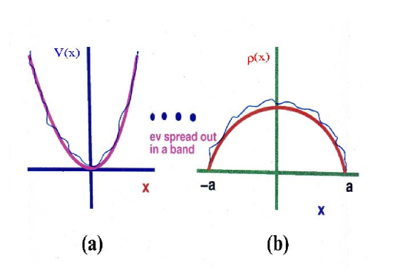
Figure 1: (a). The confining potential (b). The density of eigenvalues

On changing the potential more drastically by having two humps or wells, the simplest example being a potential $V(M)=-{\mu\over 2}M^{2}+{g\over 4}M^{4}$, the density can get disconnected support. The precise expressions for the density of eigenvalues are as follows:

$$\rho(x) = {g\over\pi}x\sqrt{(x^{2}-a^{2})(b^{2}-x^{2})}~{}~{}~{}~{}~{}~{}~{}~{}a<x<b$$ (2.1)

$$= 0~{}~{}~{}~{}~{}~{}~{}~{}-b<x<-a$$

where $a^{2}={1\over g}[|\mu|-2\sqrt{g}]$ and $b^{2}={1\over g}[|\mu|+2\sqrt{g}]$ and $|\mu|>2\sqrt{g}$, which is the condition that the wells are sufficiently deep. The eigenvalues sit in symmetric bands centered around each well. Thus $\rho$ has support on two line segments. As $|\mu|$ approaches $2\sqrt{g}$, $a\rightarrow 0$ and the two bands merge at the origin. The density is then

$$\rho(x) = {{gx^{2}}\over\pi}\sqrt{x^{2}-{2\mu\over g}}~{}~{}~{}~{}~{}~{}~{}~{}-\sqrt{2|\mu|\over g}<x<\sqrt{2|\mu|\over g}$$ (2.2)

$$= 0~{}~{}~{}~{}~{}~{}~{}~{}otherwise.$$

The phase diagram and density of eigenvalues for the $M^{4}$ potential is shown in Figs. 2.

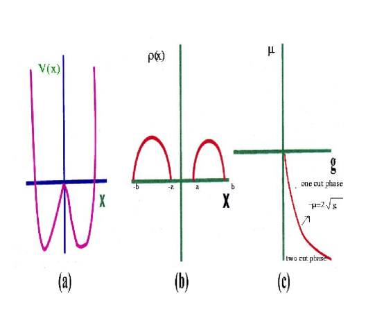
Figure 2: (a). The double-well potential (b). Density of eigenvalues (c). The phase diagram

The simplest way to determine $\rho(z)$ explicitly is to use the generating function $F(z)=<{1\over N}Tr{1\over{z-M}}>$ and its saddle point or Schwinger-Dyson equation also known in the mathematics literature as the Riemann-Hilbert problem $F(z)={1\over 2}[V^{\prime}(z)+\sqrt{\Delta}]$ with $\Delta(z)=V^{\prime}(z)^{2}-4b(z)$ and $b(z)=gz^{2}+\mu+g<{1\over N}TrM^{2}>$ (see ref. [13]). The density $\rho(x)$ is then determined by the formula $\rho(z)=-{1\over 2\pi}Im\sqrt{\Delta(z)}$.

In what follows I will outline the recurrence coefficient method of the orthogonal polynomials for the two-cut matrix model see ref. [13] for more details. I give the results for the two-point correlators (also known as the ‘smoothed’ or ‘long range’ correlators) for all three ensembles. Then the two-matrix model of Chandra-Itzykson-Zuber is defined and the expressions for the parametric and crossover correlators are given.

3 Orthogonal Polynomial Approach

The partition function $Z$, can be rewritten in terms of the orthogonal polynomials $P_{n}$ where the polynomials are defined as $\int_{-\infty}^{\infty}d\lambda e^{-NV(\lambda)}P_{n}(\lambda)P_{m}(\lambda)=h_{n}\delta_{nm}$ then $P_{n}=\lambda^{n}+l.o.$ and $P_{0}(\lambda)=1$, $P_{1}(\lambda)=\lambda+c$, $P_{2}(\lambda)=\lambda^{2}+a\lambda+b$ …… Then $Z$ the partition function in terms of the orthogonal polynomials is

$$Z=\int\prod_{i=1}^{N}d\lambda_{i}e^{-N\sum V(\lambda)}\left|\begin{array}[]{ccc}P_{0}(\lambda_{1})&....&P_{0}(\lambda_{N})\\ P_{1}(\lambda_{1})&....&P_{1}(\lambda_{N})\\ .\\ .\\ .\\ P_{N-1}(\lambda_{1})&......&P_{N-1}(\lambda_{N})\\ \end{array}\right|.$$ (3.3)

The partition function $Z$ is also known if we know the $h_{n}$’s as the partition function can be expressed in terms of the $h_{n}$’s $Z=N!h_{0}h_{1}h_{2}.....h_{N-1}.$ For example: N=2 case $\int d\lambda_{1}d\lambda_{2}e^{-NV(\lambda_{1})-NV(\lambda_{2})}(P_{0}(\lambda_{1})P_{1}(\lambda_{2})-P_{0}(\lambda_{2})P_{1}(\lambda_{1}))^{2}=h_{0}h_{1}+h_{0}h_{1}=2!h_{0}h_{1}.$ So the question is how does one find the $h$’s?

The $P_{n}$ satisfy recurrence relations

$$xP_{n}=P_{n+1}+S_{n}P_{n}+R_{n}P_{n-1}.$$ (3.4)

Note that $\int xP_{n}P_{n-2}e^{-NV(x)}dx=0$ as $xP_{n-2}=P_{n-1}+l.o.$. Thus $P_{n-2}$ $\&$ l.o. terms do not appear on the right hand side of the recurrence relation eq. (3.4). Then as $h_{n}=h_{n-1}R_{n}$ the product $h_{0}h_{1}......h_{N-1}=h_{0}(h_{0}R_{1})(h_{0}R_{1}R_{2})\\ ......(h_{0}R_{1}...R_{N})=h_{0}^{N}R_{1}^{N-1}R_{2}^{N-2}......R_{N-1}.$ The free energy $\Gamma=\ln Z=\ln N!+N\ln h_{0}+\sum_{n=1}^{N-1}(N-n)\ln R_{n}$ hence we need recurrence coefficients $R_{n}$’s to get the free energy.

4 Asymptotic Ansatz for the Orthogonal Polynomials of the Symmetric Double-Well Matrix Model

We have been able to derive in ref. [14] for the symmetric double-well matrix model the asymptotic ansatz for the orthogonal polynomials $\psi_{n}(\lambda)={P_{n}(\lambda)\over\sqrt{h_{n}}}exp(-{N\over 2}V(\lambda))$ which is

$$\psi_{n}(\lambda)={1\over{\sqrt{f(\lambda)}}}[\cos(N\zeta-(N-n)\phi+\chi+(-1)^{n}\eta)(\lambda)+O({1\over N})]$$ (4.5)

where $f$, $\zeta$, $\phi$, $\chi$ and $\eta$ are functions of $\lambda$, and $\psi_{n}$ is damped outside of the cuts. We show that $f(\lambda)={\pi\over 2\lambda}{(b^{2}-a^{2})\over 2}\sin 2\phi(\lambda)$ from the orthogonality condition satisfied by the orthogonal polynomials. $\zeta^{\prime}(\lambda)=-\pi\rho(\lambda)$ from the relation $K(\lambda,\lambda)=\rho(\lambda)$ where $K(\mu,\nu)$ is the kernel defined by ${1\over N}\sum_{i=1}^{N-1}\psi_{i}(\mu)\psi_{i}(\nu)$ and determines all eigenvalue correlators. While $\phi(\lambda)$ and $\eta(\lambda)$ are determined from the recurrence relations satisfied by the orthogonal polynomials $\cos 2\phi(\lambda)={{\lambda^{2}-({a^{2}+b^{2}\over 2})}\over{({b^{2}-a^{2}\over 2})}},$ $\cos 2\eta(\lambda)={{b\cos\phi(\lambda)}\over\lambda},$ and $\sin 2\eta(\lambda)={{a\sin\phi(\lambda)}\over\lambda}.$

$f$, $\phi$, $\eta$ and $\chi$ are universal functions independent of the potential, the only dependence on V enters through the endpoints of the cuts a and b. $\zeta$ is non-universal since the eigenvalue density depends in general on the detailed form of V. More details are to be found in the ref. [14, 15]. From this one can establish that the gapped matrix model is in a new universality class.

Using the asymptotic ansatz the full density-density correlation function maybe found and is given in ref. [14]. A simpler result are the ‘smoothed’ or ‘long range’ two-point correlation functions found in ref. [15] using a method of steepest decent which has a constant C which is undetermined unless one is explicitly in the symmetric case where $C=(-1)^{N}$ ref. [15] (ref. [17] obtain this result using a method due to Shohat), other values for C have been found earlier using the loop equation method ref. [16]. Recently in ref. [18] it was shown that for double wells with equal depths but unequal widths, in the limit of the symmetric double wells, give the value $C=(-1)^{N}$ confirming the results of ref. [15].

$$4\pi^{2}N^{2}\rho^{c}_{2}(\lambda,\mu) = {{\epsilon_{\lambda}\epsilon_{\mu}}\over{\beta\sqrt{|\sigma(\lambda)|}\sqrt{|\sigma(\mu)|}}}$$

$$\left({{\sigma(\lambda)+\sigma(\mu)}\over{(\lambda-\mu)^{2}}}+{{\sigma^{\prime}(\lambda)-\sigma^{\prime}(\mu)}\over{(\lambda-\mu)}}+\lambda^{2}+\mu^{2}-{s\over 2}(\lambda+\mu)+2C\right).$$ (4.6)

Here $\sigma(z)=(z^{2}-a^{2})(z^{2}-b^{2})$, $s=a_{1}+a_{2}+a_{3}+a_{4}$, $\epsilon_{\lambda}=+1~{}~{}for~{}~{}a_{3}<\lambda<a_{4},\epsilon_{\lambda}=-1~{}~{}for~{}~{}a_{1}<\lambda<a_{2}$ and $\beta=1,2,4$ depending on whether $M$ the matrix is real orthogonal, hermitian or self-dual quartonian. This result is different for even and odd N and hence has broken the $Z_{2}$ symmetry. It would be very interesting to be able to see this effect in experiments of mesoscopic systems which are sensitive to single electron effects.

5 The Harish Chandra-Itzykson-Zuber matrix model and density-density correlators

The two-matrix model of Harish Chandra-Itzykson-Zuber is defined by the partition function

$$Z=\int dAdBe^{-S}$$ (5.7)

where $S=NSp[V(A)+V(B)-cAB]$ and $V(A)={1\over 2}\mu A^{2}$. For $\lambda={1\over 2}$, $A$ and $B$ are $N\times N$ real symmetric matrices (orthogonal ensemble), for $\lambda=1$, $A$ and $B$ are $N\times N$ Hermitian matrices (unitary ensemble), and for $\lambda=2$ $N\times N$ real self-dual quaternions (symplectic ensemble). $Sp(A)$ stands for $TrA$ for $\lambda={1\over 2},1$ and for ${1\over 2}TrA$ for $\lambda=2$. In this model the connected density-density correlator is $\rho_{AB}(x,y)\equiv<\hat{\rho}_{A}(x)\hat{\rho}_{B}(y)>_{c}$, where the density is defined as $\hat{\rho}_{A}(x)\equiv{1\over N}Tr\delta(x-A)$, $<X>\equiv{1\over Z}\int dAdBe^{-S}X$, and the subscript $c$ implies connected part. In ref. [9] the Dyson-Schwinger equations are used to derive these eigenvalue correlators. Here only the results and physical interpretations are elaborated on.

In the large-N limit, the expectation value for the density is given by the well known Wigner semicircle law

$$<\hat{\rho}_{A}(x)>=<\hat{\rho}_{B}(x)>={2\over\pi a^{2}}\sqrt{a^{2}-x^{2}},|x|\leq a,$$ (5.8)

and $<\hat{\rho}>=0$ for $|x|\geq a$, where $a$, the “end point of the cut” is given by $a=({4\lambda\mu\over{\mu^{2}-c^{2}}})$. The result for the connected density-density correlator to leading order in ${1\over N}$, valid over the entire cut, is

$$\rho_{AB}(x,y)=-{1\over 4\pi^{2}N^{2}}{1\over\lambda a^{2}}{1\over\cos\theta\cos\alpha}\times$$

$$\left[{{1+\cosh u\cos(\theta+\alpha)}\over{[\cosh u+\cos(\theta+\alpha)]^{2}}}+{{1-\cosh u\cos(\theta-\alpha)}\over{[\cosh u-\cos(\theta-\alpha)]^{2}}}\right],$$ (5.9)

where $u\equiv ln({mu\over c})$, $|x|,|y|\leq a$, and we have defined $\sin\theta={x\over a}$ and $\sin\alpha={y\over a}$. For $\lambda=1$ the above result was derived in ref. [7] using different methods from the Dyson-Schwinger method. The Dyson-Schwinger method is capable of generalization to $\lambda={1\over 2},2$ with the above result. Then these results are relevant for the calculation of conductance fluctuation of mesoscopic systems in which the magnetic field is changing.

When one is interested in transitions from one symmetry class to another, a hamiltonian $A$ is considered consisting of two parts $B$ and $V$ each drawn from different ensembles $A=B+V$. The partition function $Z$ and action $S$ are modified to have

$$V(A)={1\over 2}\mu_{1}A^{2},~{}~{}~{}V(B)={1\over 2}\mu_{2}B^{2}$$ (5.10)

and

$$c=\mu_{1},~{}~{}~{}\mu_{2}={{\mu_{1}(1-\mu_{1}N)}\over{(2-\mu_{1}N)}}.$$ (5.11)

The constant $\mu_{1}$ measures the strength of the perturbation. At $\mu_{1}=\infty$ we get GOE, while $\mu_{1}={2\over N}$ gives GUE. However, we will work in the more general case where $\mu_{1}$, $\mu_{2}$ and $c$ are independent $O(1)$ parameters. This is just the standard two-matrix model except that A and B are drawn from different ensembles. The choice of parameters eq. (5.11), mentioned above corresponds to the crossover from GOE to GUE is then a special case of the formula derived.

We are interested in calculating the connected density-density correlator

$$\rho^{c}_{AA}(x,y)\equiv<\hat{\rho}_{A}(x)\hat{\rho}_{A}(y)>_{c}$$ (5.12)

The full smoothed global result for the connected eigenvalue correlator is (see ref. [10])

$$\rho^{c}_{AA}(x,y)=\rho^{I}_{AA}(x,y)+\rho^{II}_{AA*}(x,y)$$ (5.13)

where we find

$$\rho^{I}_{AA}(x,y)=-{1\over 2\pi}{1\over{N^{2}(x-y)^{2}}}{(a^{2}-xy)\over[(a^{2}-x^{2})(a^{2}-y^{2})]^{1\over 2}}$$ (5.14)

and

$$\rho^{II}_{AA*}(x,y)={{c^{2}\mu_{1}^{2}}\over{N^{2}(2\mu_{1}\mu_{2}-c^{2})}}[{{\cos(\phi-\theta)-1}\over{2\cos\phi\cos\theta}}\times$$

$${{2\mu_{1}^{2}(x-y)^{2}-{8\over a^{2}}(\cos 2\phi+\cos 2\theta-2\cos(\theta+\phi))-{8\mu_{1}\over a}(x-y)(\sin\theta-\sin\phi)}\over{(\mu_{1}^{2}(x-y)^{2}+{8\over a^{2}}(1-\cos(\theta-\phi))-{4\mu_{1}\over a}(x-y)(\sin\theta-\sin\phi)^{2})}}$$

$$+{{\cos(\phi+\theta)+1}\over{2\cos\phi\cos\theta}}\times$$

$${{2\mu_{1}^{2}(x-y)^{2}-{8\over a^{2}}(\cos 2\phi+\cos 2\theta+2\cos(\theta+\phi))-{8\mu_{1}\over a}(x-y)(\sin\theta-\sin\phi)}\over{(\mu_{1}^{2}(x-y)^{2}+{8\over a^{2}}(1+\cos(\theta+\phi))-{4\mu_{1}\over a}(x-y)(\sin\theta-\sin\phi)^{2})}}]$$ (5.15)

where we have used $\sin\theta={x\over a}$, $\sin\phi={y\over a}$ and $a^{2}={4\over\alpha}$. After some algebra we notice that for $\mu_{1}=\infty$,

$$\rho^{c}_{AA}(x,y)={-1\over{\pi^{2}N^{2}(x-y)^{2}}}$$ (5.16)

which is the GOE result and for $\mu_{1}={2\over N}$,

$$\rho^{c}_{AA}(x,y)={-1\over{2\pi^{2}N^{2}(x-y)^{2}}}$$ (5.17)

the GUE result. The expression eq. (5.15) is relevant for crossover from the GOE to GUE ensemble. One application of these correlation functions is to disordered mesoscopic systems using the transmission matrix formalism and the other is in the study of unoriented random surfaces.

6 Conclusions

In conclusion we have presented two classes of random matrix models. One in which there are gaps in the eigenvalue distribution and the other in which there are two coupled matrices drawn from the three ensembles (matrices taken from the same and different ensemble have been considered). In each of the models we have derived eigenvalue correlators particularly density-density correlators. In the first case of gapped matrix models we have eigenvalue correlators which dependent on $N$ the size of the matrix. This behaviour persists in the large N thermodynamic limit and for the symmetric double-well matrix model parity effects are present. For the coupled matrix models long range smoothed correlators are found. These are the parametric and crossover correlators which maybe found in mesoscopic experiments. Density-density correlators are applicable in calculations of conductance fluctuations of mesoscopic conductors. Our results in these models are valid for all eigenvalues near the center as well as the edge of the semi-circle. The behavior near the edge of the cut is particularly relevant in studies of transport properties of mesoscopic conductors ref. [6]. Thus clever mesoscopic experiments should be devised which will show the effects found in both types of these matrix models.

7 Acknowledgments

My best wishes and thanks to Professor N. Kumar on the occasion of the NKFEST. Thanks to E. Brézin, S. Jain and B. S Shastry for encouragement and collaborations.

email:ndeo@vsnl.net, ndeo@rri.res.in.

References

- [1]
- [2] M. L. Mehta Random matrices (Academic Press, 1991), T. Guhr, A. Mueller-Groeling and H. A. Weidenmueller, Phys. Rep. 299, 189, (1998).
- [3] E. Brezin and A. Zee, Nucl. Phys. B402 (613) 1993.
- [4] B. D. Simons, P. A. Lee and B. L. Altshuler, Phys. Rev. Lett. 70 (4122) 1993; Nucl. Phys. B409 (487) 1993.
- [5] O. Narayan and B.S. Shastry, Phys. Rev. Lett. 71 (2106) 1993.
- [6] C.W.J. Beenakker, Nucl. Phys. B422 (515) 1994; Phys. Rev. Lett. 70 (1155) 1993.
- [7] E. Brézin and A. Zee, Nucl. Phys. B424[FS] (435) 1994, Phys. Rev. E 49 (2588) 1994.
- [8] A. Pandey, Chaos, Solitons and Fractals 5, 1275, 1995.
- [9] N. Deo, S. Jain and B. S. Shastry, Phys. Rev. E 52 (4836) 1995.
- [10] N. Deo, Nucl. Phys. B464[FS] (463) 1996.
- [11] S. Jain, Mod. Phys. Lett. A 11 (1201) 1996.
- [12] Harish Chandra, Amer. J. Math 80 241 (1958), C. Itzykson and J. B. Zuber, J. Math. Phys. 21 411 (1980).
- [13] R. C. Brower, N. Deo, S. Jain and C. I. Tan, Nucl. Phys. B405 (166) 1993.
- [14] N. Deo, Nucl. Phys. B504 (609) 1997.
- [15] E. Brezin and N. Deo, Phys. Rev. E 59 (3901) 1999.
- [16] G. Akemann and J. Ambjorn, J. Phys. A29 (L555) 1996, G. Akemann, Nucl. Phys. B482 (403) 1996 and Nucl. Phys. B507 (475) 1997.
- [17] E. Kanzieper and V. Freilikher, Phys. Rev. E 57 (6604) 1998.
- [18] G. Bonnet, F. David and B. Eynard, J. Phys. A 33 (2000) 6739.