Projected wave functions for fractionalized phases of quantum spin systems

Abstract

Gutzwiller projection allows a construction of an assortment of variational wave functions for strongly correlated systems. For quantum spin $S=1/2$ models, Gutzwiller-projected wave functions have resonating-valence-bond structure and may represent states with fractional quantum numbers for the excitations. Using insights obtained from field-theoretical descriptions of fractionalization in two dimensions, we construct candidate wave functions of fractionalized states by projecting specific superconducting states. We explicitly demonstrate the presence of topological order in these states.

I Introduction

In the last several years, considerable theoretical progress has been made in understanding the possibility of fractional quantum numbers for the excitations of strongly interacting systems. A particular focus of attention has been on realizing such phases in quantum spin systems in two spatial dimensions[1]. In conventional quantum phases of spin-$1/2$ magnets, such as an antiferromagnet or a spin-Peierls phase, the spin excitations carry quantum numbers $S=1$ or higher multiples. In contrast, in a fractionalized phase, there are excitations (dubbed spinons) that carry spin $S=1/2$. Various kinds of evidence for the presence of such fractionalized phases in spin models on a number of diverse lattices have been presented in Ref. [2]. A detailed theoretical study[3, 4, 5, 6, 7, 8] of fractionalization in two dimensions has revealed that in the simplest cases such spinon excitations are necessarily accompanied by gapped “vortex”-like excitations: visons. The visons carry no spin but have a long-range statistical interaction with the spinon: When a spinon is taken all the way around a vison, the wave function of the system changes sign. Thus the visons have an Ising-like character: two visons can annihilate each other and are equivalent to no vison at all. A concise mathematical description of this long ranged statistical interaction is given by assigning a $Z_{2}$ gauge charge to the spinons and a corresponding $Z_{2}$ gauge flux to the visons.

A precise theoretical characterization[4, 9] of fractionalized phases serving to distinguish them from more conventional phases is provided by the notion of topological order — a concept elucidated by Wen[10] in his work on the quantum Hall effect. When placed on a manifold with a non-trivial topology, a fractionalized phase has a number of locally similar but globally distinct states that differ by whether or not a vison threads each hole of the manifold.

If a spin model possesses a fractionalized phase, what does its wave function look like in terms of the original spins? In this paper, we argue that the wave functions describing a fractionalized state may be obtained from the original RVB construction of Anderson[1]. We consider states obtained by projecting the wave function of a BCS superconductor (on a lattice) to the Hilbert space of exactly one electron per site (this procedure is also known as Gutzwiller projection[11]). Different topological sectors are obtained by projecting states with/without superconducting vortices (or, equivalently, with different boundary conditions). We motivate this construction from the field-theoretic description of fractionalized phases.

Projected wave functions have long been studied[12, 13, 14] to gain insight into the properties of the cuprate materials. However, as we show below, it is not guaranteed that the resulting wave function describes any fractionalized phase. The state that has been the subject of most attention is the “$d$-wave RVB state” obtained by projecting a BCS $d_{x^{2}-y^{2}}$ superconductor with nearest neighbor hopping and nearest neighbor pairing interactions. We argue below that such a superconducting state has some special symmetry properties due to which it is not expected to lead to a fractionalized state after projection (at half-filling). We confirm this by a direct numerical calculation on this state. It is not clear whether the nearest neighbor $d$-wave RVB state represents a good trial wave function for any stable phase of a spin system. Addition of a number of perturbations, such as for instance next-nearest-neighbor hopping, to the nearest-neighbor $d$-wave superconductor removes the special symmetry properties — the resulting state is then expected to lead, after projection, to a fractionalized state. We demonstrate explicitly the topological order in such projected states. A closely related state was recently considered in Ref. [15] at finite doping and was argued to provide a good description of cuprate phenomenology. We note that recent experiments[16, 17] place constraints on the applicability of fractionalization ideas to the cuprates. Theoretical description of the cuprates with wave functions corresponding to fractionalized states must hence be performed with caution and examined for consistency with experiments.

Recently, a particular projected state has been argued to represent the ground state of the $J_{1}-J_{2}$ Heisenberg model on the square lattice[18]. We argue that such a state is also expected to have topological order, and hence be fractionalized. We explicitly construct four globally distinct states on the torus to demonstrate the topological order.

If the projection does indeed lead to a fractionalized state, then we may construct wave functions for its excitations as follows. The distinct excitations of a superconductor are the BCS quasiparticles and the vortices. As originally suggested by Anderson[1], projection of the BCS quasiparticles directly leads to the spinons. We argue that the visons may be obtained by projecting the wave function of the BCS $hc/2e$ vortex. This observation may be directly exploited to check for topological order in the projected wave functions. Consider putting the system on a torus. We may project the four superconducting states obtained by threading or not threading a $hc/2e$ vortex through each hole of the torus. If the projected state is fractionalized, and hence topologically ordered, these four states must be (after projection) orthogonal to each other in the thermodynamic limit though they are locally similar.

II Generalities on Gutzwiller projection

The original point of view on the Gutzwiller projected wave function[1] is that it describes a state obtained by quantum disordering a Heisenberg Neel antiferromagnet. However, as Gutzwiller projection (at half filling) freezes out the charge fluctuations inherent in the unprojected superconducting state, it may equally well be viewed as describing a state obtained by quantum disordering a superconductor. Recent theoretical work[6, 7] has sought to understand the properties of Mott insulators by viewing them as quantum disordered superconductors. In this approach, insulating phases are regarded as condensates of the vortices of the superconductor. A fractionalized Mott insulator is obtained by pairing and condensing the BCS vortices while the unpaired $hc/2e$ vortex remains gapped. At energy scales well below the charge gap, the excitations in such a Mott insulator are the spinon and the vison. The spinons are precisely what become of the fermionic BCS quasiparticles once the $hc/e$ vortices condense. The vison on the other hand is the remnant of the unpaired $hc/2e$ vortex - due to the $hc/e$ condensate, this survives with only a $Z_{2}$ character.

It is clear that this point of view fits in nicely with the idea of Gutzwiller projecting superconducting states to obtain wave functions for Mott insulators. However not all choices of the unprojected superconducting state are guaranteed to lead to fractionalized states on projection (see Sections below). In this section, we discuss the nature of projected vortex states and their use in constructing the wave function of the vison.

A RVB wave functions

We begin by quickly reviewing the interpretation of the Gutzwiller-projected superconducting state as a resonating valence bond wave function. Consider the ground state of a BCS Hamiltonian on a $L\times L$ square lattice ($L$ even):

$$H=-\sum_{ij}\sum_{\alpha}t_{ij}c^{\dagger}_{i\alpha}c_{j\alpha}+{\rm h.c.}+\Delta_{ij}c^{\dagger}_{i\uparrow}c^{\dagger}_{j\downarrow}+{\rm h.c.}$$ (1)

Its wave function has the form

$$\left|BCS\right\rangle=\prod_{\vec{k}}\left(u_{\vec{k}}+v_{\vec{k}}c^{\dagger}_{\vec{k}\uparrow}c^{\dagger}_{-\vec{k}\downarrow}\right)\left|0\right\rangle$$ (2)

in standard notation. We restrict attention to spin-singlet, time-reversal-invariant ground states that also preserve all the symmetries of the lattice. The vectors $\vec{k}$ take values in the first Brillouin zone. We assume periodic boundary conditions in both spatial directions so that $\vec{k}=\frac{2\pi}{L}(m_{x},m_{y})$ with $m_{x},m_{y}$ integers (the system may be thought of as residing on a torus). We may rewrite this wave function as

$$\left|BCS\right\rangle\propto\exp\left({\sum_{k}g(\vec{k})c^{\dagger}_{\vec{k}\uparrow}c^{\dagger}_{-\vec{k}\downarrow}}\right)\left|0\right\rangle$$ (3)

with $g(\vec{k})=v_{\vec{k}}/u_{\vec{k}}$. So long as $g(\vec{k})=g(-\vec{k})$, this state is guaranteed to be a spin singlet.

It will be useful to consider a first quantized version $\Psi(\{\vec{x}_{i},\chi_{i}\})$ obtained by fixing the total number of particles to be $L^{2}$. The $(\vec{x}_{i},\chi_{i})$ are the position and spin state of the $i$’th electron. We have

$$\Psi(\{\vec{x}_{i},\chi_{i}\})\propto\left\langle\{\vec{x}_{i},\chi_{i}\}\right|\left(\sum_{k}g_{\vec{k}}c^{\dagger}_{\vec{k}\uparrow}c^{\dagger}_{-\vec{k}\downarrow}\right)^{L^{2}/2}\left|0\right\rangle$$ (4)

The wave function $\Psi(\{\vec{x}_{i},\chi_{i}\})$ is single-valued on the torus.

The Gutzwiller-projected state $\left|RVB\right\rangle$ is obtained by projecting $\Psi$ further onto a subspace where there is exactly one particle per lattice site. The resulting wave function may be written as a sum over various valence-bond configurations on the lattice:

$$\left|RVB\right\rangle=P_{G}\left|BCS\right\rangle\propto\sum_{vbc}{\cal A}_{vbc}\left|vbc\right\rangle$$ (5)

where $\left|vbc\right\rangle$ denotes any particular valence bond covering. ${\cal A}_{vbc}$ is the corresponding amplitude and is given by the product of $g(\vec{x}_{i}-\vec{x}_{j})$ over all valence bonds connecting sites $(ij)$ appearing in the state $\left|vbc\right\rangle$. Here $g(\vec{x}_{i}-\vec{x}_{j})$ is the Fourier transform of the function $g(\vec{k})$ introduced above.

B BCS vortices and their projections

If the ground state of a spin system is correctly described by Gutzwiller projecting a BCS state, it is natural to construct excitations of the spin system by similarly projecting the excitations of the BCS superconductor. As argued by Anderson, projecting the BCS quasiparticle state leads to a wave function for neutral spin-$1/2$ spinons. The other distinct excitations of the superconductor are the vortices. What happens to these under the Gutzwiller projection? To answer this question, consider a wave function of a superconductor describing a state where a $nhc/2e$ vortex threads the torus along the $x$-direction. If $n$ is even, the (first-quantized) wave function may be taken simply as

$$\Psi_{n_{x}}=\exp\left({\sum_{i}\frac{in\theta_{i}}{2}}\right)\,\Psi$$ (6)

where $\theta_{i}=\frac{2\pi y_{i}}{L}$ is the angular coordinate of the $i$’th particle. Thus, the vortex wave function for even $n$ may be simply obtained by multiplying the ground state wave function by a phase factor (which depends on the configuration of the particles). Upon Gutzwiller projection, there is one particle at every site; consequently the projected vortex state (for $n$ even) is trivially related to the projected ground state by an overall phase factor. Thus the projected even vortex state does not lead to a distinct state of the spin system.

For $n$ odd, the vortex wave function in the superconductor is not obtained by simply multiplying the ground state by a phase factor. Consider $n=1$. The naive guess

$$\exp\left({\sum_{i}\frac{i\theta_{i}}{2}}\right)\,\Psi$$ (7)

violates the physical requirement that all legitimate electron wave functions must be single-valued on the torus. The correct wave function is constructed by multiplying by the phase factor above, and replacing $\Psi$ by a wave function that satisfies antiperiodic boundary conditions along the $y$-direction (and periodic along the $x$-direction). Such a replacement may be obtained by considering the ground state of $H$ with antiperiodic boundary conditions along the $y$-direction:

$$\left|BCS^{+-}\right\rangle=\prod_{k}\left(u_{\vec{k}^{\prime}}+v_{\vec{k}^{\prime}}c^{\dagger}_{\vec{k}^{\prime}\uparrow}c^{\dagger}_{-\vec{k}^{\prime}\downarrow}\right)\left|0\right\rangle$$ (8)

with $\vec{k}^{\prime}=\vec{k}+\frac{\pi}{L}\hat{y}$ and $\vec{k}=\frac{2\pi}{L}(m_{x},m_{y})$ as before. Multiplying by the phase factor above has the effect of shifting all the momenta by $\frac{\pi}{L}$ along the $y$-direction. A legitimate $hc/2e$ vortex state may therefore be constructed as

$$\left|BCS^{\prime}\right\rangle=\prod_{k}\left(u_{\vec{k}^{\prime}}+v_{\vec{k}^{\prime}}c^{\dagger}_{\vec{k}+\frac{2\pi\hat{y}}{L}\uparrow}c^{\dagger}_{-\vec{k}\downarrow}\right)\left|0\right\rangle$$ (9)

It is readily verified that this is a spin-singlet wave function. The first quantized $hc/2e$ vortex wave function (with $L^{2}$ particles) may now be obtained straightforwardly as

$$\Psi^{\prime}\propto\left\langle\{\vec{x}_{i},\chi_{i}\}\right|\left(\sum_{\vec{x},\vec{x}^{\prime}}g^{\prime}(\vec{x},\vec{x}^{\prime})c^{\dagger}_{\uparrow}(\vec{x})c^{\dagger}_{\downarrow}(\vec{x}^{\prime})\right)^{L^{2}/2}\left|0\right\rangle$$ (10)

with

$$g^{\prime}(\vec{x},\vec{x}^{\prime}) = e^{i\frac{\pi}{L}(y+y^{\prime})}g_{a.p}(\vec{x}-\vec{x}^{\prime}),$$ (11)

$$g_{a.p}(\vec{x}-\vec{x}^{\prime}) = \sum_{\vec{k}^{\prime}}g(\vec{k}^{\prime})e^{i\vec{k}^{\prime}.(\vec{x}-\vec{x}^{\prime})}$$ (12)

$$= \sum_{\vec{k}^{\prime}}g(\vec{k}^{\prime})\cos\left(\vec{k}^{\prime}.(\vec{x}-\vec{x}^{\prime})\right)$$ (13)

Here, as before, $g(\vec{k}^{\prime})=\frac{u_{\vec{k}^{\prime}}}{v_{\vec{k}^{\prime}}}$. The function $g_{a.p}(\vec{x}-\vec{x}^{\prime})$ satisfies antiperiodic boundary conditions along the $y$ direction, and periodic along the $x$ direction:

$$g_{a.p}(\vec{r}+L\hat{y}) = -g_{a.p}(\vec{r})$$ (14)

$$g_{a.p}(\vec{r}+L\hat{x}) = g_{a.p}(\vec{r})$$ (15)

This vortex state may now be projected to obtain the new RVB wave function given by

$$\left|RVB^{\prime}\right\rangle=P_{G}\left|BCS^{\prime}\right\rangle\propto\sum_{vbc}{\cal A}^{\prime}_{vbc}\left|vbc\right\rangle$$ (16)

The amplitude ${\cal A}^{\prime}_{vbc}$ is given by the product of $g^{\prime}(\vec{x}_{i}-\vec{x}_{j})$ over all valence bonds connecting sites $i$ and $j$ appearing in the state $\left|vbc\right\rangle$. This wave function can be further simplified by noting that the factor $\exp({i\frac{\pi}{L}\sum_{i}y_{i}})$ arises in every term on the right-hand side and is just a trivial multiplication by an overall phase factor, and hence may be dropped. (For an $L\times L$ square lattice with $L$ even, this phase factor is simply equal to one). This then amounts to Gutzwiller projecting the state $\left|BCS^{+-}\right\rangle$ obtained by changing the boundary conditions on the unprojected state. The resulting amplitude for a valence bond $(ij)$ is given by $g_{a.p}(\vec{x}_{i}-\vec{x}_{j})$.

Thus the projection of a $hc/2e$ vortex potentially survives as a non-trivial state in the spin system. In view of the discussion at the beginning of this section, it is clear that if the ground state described by $\left|RVB\right\rangle$ is indeed fractionalized, then $\left|RVB^{\prime}\right\rangle$ describes a state with a vison threaded through along the $x$-direction. We will exploit this observation below to check for topological order in the projected wave functions.

C Short ranged RVB states and dimer models

It is instructive to make a short digression, and specialize to superconducting states which are fully gapped, and where the function $g(\vec{r})$ has a very short range of order a few lattice spacings. In that case, the resulting RVB wave function describes a state with only short ranged valence bonds (and presumably a full spin gap). For such a state, it is expected that the function $g(\vec{k})$ is smooth in $\vec{k}$-space so that we may approximate $g(\vec{k}^{\prime})\approx g(\vec{k})$. In real space, this amounts to

$$g_{a.p}(\vec{x}-\vec{x}^{\prime})\approx g(\vec{x}-\vec{x}^{\prime})\cos\left(\frac{\pi}{L}(y-y^{\prime})\right)$$ (17)

In the limit of large $L$, the cosine factor is one everywhere except for valence bonds that connect sites to the left of $y=L$ to sites to the right of $y=L$ for which it is $-1$. Thus the difference between the projected ground state and the projected $hc/2e$ state may be summarized as follows: Consider drawing a vertical line parallel to the $x$-direction that cuts all the links of the lattice between $y=L$ and $y=1$. In the projected vortex state, the amplitude for any valence bond that cuts this line acquires a factor $(-1)$ relative to the ground state. In other words, the amplitude for any valence bond configuration where an odd number of valence bonds intersect this line is $(-1)$ relative to the ground state. We note that this construction of the projected vortex wave function reduces to the state considered by Read and Chakraborty in their pioneering early work[19] on topological order in RVB wave functions. Unfortunately, as already recognized in that paper[19] it is not clear that the particular RVB state discussed there describes any stable phase of a spin system.

An approximate description of a short ranged RVB state is through a quantum dimer model[20]. It is well-known[20, 21] that the quantum dimer model on a torus has four distinct topological sectors classified by whether the number of dimers intersecting particular lines similar to the one introduced above is even or odd. Fractionalization in the original spin model is signalled by topological order in the quantum dimer model when the four topological sectors become degenerate in energy. In this case, these even/odd sectors clearly correspond to the symmetric/antisymmetric combination of the state with no vison and a threaded vison. This is completely consistent with our construction of the vison wave function by projecting the $hc/2e$ vortex.

Our primary interest in this paper will be long-ranged RVB states where the spinons are gapless. We will explore the properties of wave functions for such states by numerical calculations using the construction above.

III Topological order: general considerations

Though the projected $hc/2e$ vortex survives as a non-trivial state of the spin system, it is still not necessary that the state $\left|RVB\right\rangle$ has topological order. The presence or lack thereof of topological order may be established by examining the following two conditions:

(i) $\langle RVB^{\prime}|RVB\rangle=0$ as the system size goes to infinity, and

(ii) The expectation values of all local physical operators be the same in both states $\left|RVB\right\rangle$ and $\left|RVB^{\prime}\right\rangle$ again in the thermodynamic limit.

The first condition is closely related to the presence of a vison gap in the bulk. Indeed, the states $|RVB\rangle$ and $|RVB^{\prime}\rangle$ differ by one vison tunneled across the cylinder (or torus), and therefore $\langle RVB|RVB^{\prime}\rangle$ may be interpreted as the amplitude of such a tunneling event. The second condition guarantees that the distinction between the states is not in any local properties but rather in global ones. In this section, we will examine some simple arguments that motivate the choice of particular superconducting wave functions which will lead to fractionalized states on projection.

Consider the first condition. It is easy to check that the overlap $\langle BCS^{\prime}|BCS\rangle$ goes to zero very rapidly as $L$ becomes large. This is expected physically as the vorticity is a good quantum number for the unprojected BCS state. However, this does not guarantee $\langle RVB^{\prime}|RVB\rangle=0$ due to the projection. To get better insight into what is needed for condition (i) to be satisfied, we will employ the following useful characterization of the Gutzwiller projection. In the unprojected Hilbert space, the states at each site are $\left|0\right\rangle,\left|\uparrow\right\rangle,\left|\downarrow\right\rangle,\left|\uparrow\downarrow\right\rangle$ in obvious notation. Projection keeps only the states $\left|\uparrow\right\rangle,\left|\downarrow\right\rangle$ at each site. At each site $i$, introduce the physical spin operator $\vec{S}_{i}$ and the pseudo-spin operator $\vec{T}_{i}$:

$$\vec{S}_{i} = \frac{1}{2}c^{\dagger}_{i}\vec{\sigma}c_{i}$$ (18)

$$T^{z}_{i} = \frac{c^{\dagger}_{i}c_{i}-1}{2}$$ (19)

$$T^{+}_{i} = c^{\dagger}_{i\uparrow}c^{\dagger}_{i\downarrow}$$ (20)

$$T^{-}_{i} = c_{i\downarrow}c_{i\uparrow}$$ (21)

Here $T^{\pm}_{i}=T^{x}_{i}\pm T^{y}_{i}$. The $\vec{T}_{i}$ satisfy $SU(2)$ commutation relations just like the physical spin operators $\vec{S}_{i}$. Furthermore, all components of $\vec{T}_{i}$ commute with all components of $\vec{S}_{i}$. Clearly the states $\left|\uparrow\right\rangle,\left|\downarrow\right\rangle$ are singlets under the pseudo-spin rotation generated by the $\vec{T}_{i}$, while the states $\left|0\right\rangle,\left|\uparrow\downarrow\right\rangle$ form a doublet under the pseudospin rotation. Thus the Gutzwiller projection is equivalent to projection onto the singlet sector (at each site) of the pseudospin $SU(2)$ rotation. This has the general implication

$$P_{G}\left|\psi_{\rm unproj}\right\rangle=P_{G}U\left|\psi_{\rm unproj}\right\rangle$$ (22)

for an arbitrary $SU(2)$ rotation

$$U=e^{i\sum_{i}\vec{\theta}_{i}.\vec{T}_{i}}$$ (23)

where the parameters $\vec{\theta}_{i}$ may be chosen independently on each site. Thus a local pseudospin $SU(2)$ rotation of the unprojected state does not change the state after projection. We will therefore call this a gauge rotation.

In view of the above, a sufficient condition for the orthogonality of $\left|RVB\right\rangle$ and $\left|RVB^{\prime}\right\rangle$ is simply

$$\langle BCS|U|BCS^{\prime}\rangle=0$$ (24)

for any arbitrary pseudospin $SU(2)$ rotation (23). (We note that this is not in general a necessary condition for the orthogonality).

The discussion has so far been general. Eqn. (24) imposes some conditions on the nature of the BCS state which could lead to a wave function for a fractionalized state after projection. However Eqn. (24) is still not in a form which is directly useful in providing guidance in writing down such states. To get a more useful form, we specialize to a particular class of unprojected states. In general, the state $\left|BCS\right\rangle$ will be a linear superposition of states with different total particle number. On the other hand, the projected state $\left|RVB\right\rangle$ has exactly one particle per site, and hence an exact total of $L^{2}$ particles on a lattice with $L^{2}$ sites. Now, for a general BCS state, if we plot the probability distribution of having a total of $n$ particles, it will have a sharp peak at some average value $n_{0}$ and will die rapidly for $|n-n_{0}|$ large. If $n_{0}$ is different from $L^{2}$, then the Gutzwiller projection picks out the tails of the original BCS wave function. In this case, the projected wave function may have very little to do with the unprojected one. For the projected state to retain the significant features of the spin physics of the unprojected state, it is clearly advantageous[22] to require that the mean number of particles (before projection) is $L^{2}$. If this is satisfied, the projection will have a gentler effect than if the mean number is different from one per site. To further soften the effect of the projection, it is clearly advantageous to require that the mean number be one for every unprojected state obtained from $\left|BCS\right\rangle$ by a pseudospin $SU(2)$ gauge rotation. This ensures that the projection does not pick up the tails of the wave function in any gauge.

The requirement that the average electron number on each site is one may be simply written as

$$\langle T_{i}^{z}\rangle=0$$ (25)

on all sites $i$. Further the requirement that this be true for every gauge-rotated ground state is equivalent to requiring that

$$\langle\vec{T}_{i}\rangle=0,$$ (26)

i.e. the average values of the generators of the gauge rotations vanish.

From now on, we will specialize to unprojected states where the requirement Eqn. (26) is satisfied. In this case, we may hope that we can use our intuition about the unprojected state to infer the properties of the projected state. When do we expect that Eqn. (24) will be satisfied for such a BCS state? Note that $\left|BCS^{\prime}\right\rangle$ differs from $\left|BCS\right\rangle$ in having a $hc/2e$ vortex threaded through the hole of the cylinder. If the ground state of a physical system is given by the superconducting state $\left|BCS\right\rangle$, we can label it’s excitations by their total vorticity quantum number. The state $\left|BCS^{\prime}\right\rangle$ has total vorticity $\pm 1$ compared to $\left|BCS\right\rangle$, and hence is orthogonal. However, so long as $U\left|BCS\right\rangle$ is also a superconducting state, it will also have a fixed vorticity which differs from that of $\left|BCS^{\prime}\right\rangle$ by an odd number. Consequently, in this case Eqn. (24) will be satisfied. If however for some $U$, the gauge rotated state $U\left|BCS\right\rangle$ is not a superconducting state, then it may be regarded as a coherent superposition of electron wave functions each of which carry a definite vorticity. (The vorticity is not a good quantum number in a non-superconducting state). It is then possible that $\left|BCS^{\prime}\right\rangle$ is not orthogonal to that particular gauge rotated state, so that Eqn. (24) is not satisfied. At the very least, we lose the general reason requiring orthogonality.

Based on the reasoning above, we make the following conjecture:

An unprojected state where the constraint (26) is satisfied, and which cannot be rotated to a non-superconducting state by an $SU(2)$ gauge rotation, will lead to a topologically ordered state after projection.

This conjecture provides strong motivation for choosing particular superconducting states that we may project to obtain topologically ordered states. On the other hand, we do not provide any formal proof of this conjecture in this paper. It is supported by the reasoning in this section, and by our numerical results.

Here we need to make a clear distinction between “superconducting” and “non-superconducting” states. Formally, we call a state “gauge-equivalent to non-superconducting” if it is invariant under a global $U(1)$ subgroup of the full group of gauge rotations (23). Indeed, a non-superconducting state is characterized by a fixed number of electrons. Then the $U(1)$ group of global rotations by $T^{z}$ (i.e., the subgroup generated by the sets $\vec{\theta}_{i}=\theta\hat{z}$) produces only trivial multiplications by phase factors leaving the state invariant. We call such a state a “$U(1)$ state” [or even a “$SU(2)$ state” in the case when the maximal subgroup leaving the unprojected state invariant is $SU(2)$]. In this terminology, a state that is superconducting in any gauge is called a “$Z_{2}$ state”. This classification is a sub-classification of a more detailed one introduced by Wen[23].

A set of conditions for the $U(1)$ invariance (being gauge-equivalent to non-superconducting) of a given state may be formally written in terms of projector operators onto occupied quasiparticle states. Consider the set of Bogoliubov–deGennes doublets $(u_{\vec{k}},v_{\vec{k}})$ participating in the ground state (2). We can define a projector onto the linear subspace spanned by those doublets. In real space, this projector may be thought of as a set of $2\times 2$ matrices $P_{ij}$ labeled by the site indices $i$ and $j$ and defined as

$$P_{ij}=\sum_{\vec{k}}\pmatrix{u_{\vec{k}}(i)\cr v_{\vec{k}}(i)}\pmatrix{u_{\vec{k}}^{*}(j)&v_{\vec{k}}^{*}(j)}$$ (27)

Under the $SU(2)$ gauge transformation, these matrices transform as

$$P_{ij}\rightarrow U_{i}P_{ij}U^{\dagger}_{j}$$ (28)

For a non-superconducting state, all matrices $P_{ij}$ are simultaneously diagonal. To see when a given state can be gauge rotated to such a non-superconducting state, it is useful to consider the chain products of such matrices starting and ending at the same point $i$:

$$A_{i}[C]=\Pi_{C}\left(P_{ij}P_{jk}\dots P_{li}\right)$$ (29)

where $(i,j,k,\dots,l,i)$ define a closed curve on the lattice. $A_{i}[C]$ is a $2\times 2$ matrix for each lattice site $i$ and for each closed curve $C$ starting and ending at that site. Now one easily verifies that all matrices $P_{ij}$ may be simultaneously diagonalized if and only if for any $i$ and for any pair of closed contours $C$ and $C^{\prime}$ both starting and ending at $i$,

$$\left[A_{i}[C],A_{i}[C^{\prime}]\right]=0$$ (30)

Thus to check that a given wave function describes a $Z_{2}$ state (i.e. cannot be gauge rotated to a non-superconducting form), it is sufficient to verify that $A_{i}[C]$ and $A_{i}[C^{\prime}]$ do not commute for at least one choice of $i$, $C$, and $C^{\prime}$.

Instead of checking whether the wave function may be rotated to a non-superconducting form, one may perform a similar test for the Hamiltonian (1). The Hamiltonian can be rotated to a non-superconducting one (i.e containing no pairing terms) if and only if

$$\left[B_{i}[C],B_{i}[C^{\prime}]\right]=0,$$ (31)

for all $i$ and $C$, where

$$B_{i}[C]=\Pi_{C}\left(H_{ij}H_{jk}\dots H_{li}\right),\quad H_{ij}=\pmatrix{t_{ij}&\Delta_{ij}\cr\Delta^{*}_{ij}&-t^{*}_{ij}}$$ (32)

This is a convenient sufficient condition for being a $U(1)$ wave function, but not a necessary one: in certain cases, a superconducting Hamiltonian may have a non-superconducting ground state (with a definite particle number).

It is instructive to consider some specific examples of superconducting states to see how these conditions work in practice. Consider for instance a nearest neighbor $d$-wave superconductor where $t_{ij},\Delta_{ij}$ are non-zero only on nearest-neighbor bonds, and take the values

$$t_{ij} = t$$ (33)

$$\Delta_{ij} = \pm\Delta.$$ (34)

The plus sign in the second equation is for horizontal bonds, and the minus sign for vertical bonds. It is readily seen that the condition in Eqn. (26) is satisfied by this state. However, as is also easily seen, all the $B_{i}[C]$ commute for this state. This is of course consistent with the well-known fact that this state can be gauge rotated to a pure hopping state (known as the staggered flux state). We therefore expect that this state will not lead to a fractionalized state after projection. This is confirmed by our numerical calculations below.

Now consider adding the next-near-neighbor diagonal hopping $t^{\prime}$ to this state. The resulting Hamiltonian still describes a $d_{x^{2}-y^{2}}$ superconductor. However, a simple calculation shows that there are two non-commuting $B_{i}[C]$ matrices so that this can no longer be rotated to pure hopping. Addition of $t^{\prime}$ changes the mean density away from one particle per site. This can however be compensated by adding an on-site chemical potential term to the unprojected Hamiltonian. The state thus constructed is therefore a good candidate for projecting to get a wave function for a fractionalized state. Below, in Section IV we demonstrate this by a numerical calculation.

Surprisingly, the criteria obtained above for the superconducting state to describe a topologically ordered state after projection may also be motivated from a completely different point of view[4, 23]. Consider any spin $S=1/2$ model in two dimensions. As is well-known, it is possible to use a representation of the spins in terms of fermionic spin-$1/2$ operators. This representation is exact so long as the constraint that the fermion occupation is one at each site is imposed on the Hilbert space. A popular approach is to treat the resulting fermion Hamiltonian in mean field theory. At the mean-field level, the excitations are neutral spin-$1/2$ fermions described by a Hamiltonian of the general form Eqn. (1). The exact constraint inherent in the fermionic representation is replaced precisely by Eqn. (26). This mean field state is capable of correctly describing a possible physical phase of the spin model as long as it is stable to fluctuations. As discussed by Wen[4, 23], the criteria for the stability of the mean field state to fluctuations are precisely that expressed in Eqn. (31). If the mean field state is indeed stable to fluctuations, then we expect that the candidate wave function for the physical state described by it is given by the Gutzwiller projection of the mean field wave function to the physical Hilbert space.

IV Numerical results

We further verify our conjecture numerically by testing the conditions (i) and (ii) of Section III on the square lattice in the toroidal geometry for several examples of the projected BCS wave functions. We label the ground states in the four topological sectors as $\left|{+}{+}\right\rangle$, $\left|{+}{-}\right\rangle$, $\left|{-}{+}\right\rangle$, and $\left|{-}{-}\right\rangle$, according to the boundary conditions imposed in $x$ and $y$ directions. We employ the variational Monte Carlo method described in detail in Ref. [13] applied to the square $L{\times}L$ tori.

FIG. 1.: The mean-field states generating the four wave functions NND, D1, D2, and DD. The terms of the Hamiltonian (1) are shown on one plaquette of the lattice. The solid lines denote hopping, the dashed lines denote pairing, and the circles around vertices denote the chemical potential.

We consider four different types of projected wave functions: the nearest-neighbor $d_{x^{2}-y^{2}}$ state and its three modifications by including hopping or pairing along the plaquette diagonals (Fig. 1). All these wave functions may be parameterized by translationally invariant Hamiltonians (1), and we can conveniently describe them in terms of the Fourier transform of $H_{ij}$ (defined above in Eq. (32)):

$$H({\bf k})=\pmatrix{\xi({\bf k})&\Delta({\bf k})\cr\Delta^{*}({\bf k})&-\xi(-{\bf k})}\,.$$ (35)

The nearest-neighbor $d_{x^{2}-y^{2}}$-wave BCS state (further denoted as NND) is defined by its kinetic and pairing amplitudes:

$$\xi({\bf k}) = -2(\cos k_{x}+\cos k_{y})\,,$$ (36)

$$\Delta({\bf k}) = \Delta_{0}(\cos k_{x}-\cos k_{y})\,.$$ (37)

In the projected NND wave function, the nearest-neighbor antiferromagnetic correlations are maximized at the intermediate value of $\Delta_{0}\approx 0.55$ [12, 24] (the optimal values of $\Delta_{0}$ reported in these two references differ by several percent; the precise value of $\Delta_{0}$ is not important for our qualitative results concerning topological order). We find that the NND state after projection has no topological order. This agrees with our conjecture, since the NND state can be rotated to the pure-hopping staggered-flux state by a SU(2) gauge rotation [25, 26].

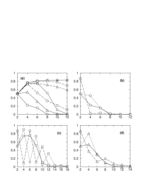
FIG. 2.: Overlaps between wave functions with different boundary conditions on tori $L\times L$ as a function of the system size $L$. All wave functions have $\Delta_{0}=0.55$. (a): overlaps $\langle{+-}|{-+}\rangle$. Stars: NND wave function. Circles: D1 wave functions (dashed line: $t^{\prime}=0.5$, $\mu=0.417$; solid line: $t^{\prime}=1.0$, $\mu=0.696$). Squares: D2 wave functions (dashed line: $t^{\prime}=0.3$, $\mu=0.509$; solid line: $t^{\prime}=0.5$, $\mu=0.794$). Triangles: DD wave functions (dashed line: $D_{xy}=0.4$; solid line: $D_{xy}=1.0$). (b): overlaps for the D1 wave function with $t^{\prime}=1.0$, $\mu=0.696$. (c): overlaps for the D2 wave function with $t^{\prime}=0.5$, $\mu=0.794$. (d): overlaps for the DD wave function with $D_{xy}=1.0$. In plots (b)–(d), solid line corresponds to $\langle{+-}|{-+}\rangle$, dashed line — to $\langle{+-}|{++}\rangle$, dotted line — to $\langle{+-}|{--}\rangle$. For these three wave functions, the overlap $\langle{++}|{--}\rangle$ is found to be zero for all system sizes, within the numerical accuracy (about 0.003).

In addition to the NND state, we consider its three modifications which are $Z_{2}$ states (cannot be gauge rotated to a non-superconducting form). In the first modification (we denote it by D1), we add hopping along one of the plaquette diagonals which amounts to replacing (36) by

$$\xi({\bf k})=-2[\cos k_{x}+\cos k_{y}+t^{\prime}\cos(k_{x}+k_{y})]-\mu\,.$$ (38)

The chemical potential $\mu$ is added for adjusting the average particle density in the unprojected wave function in order to satisfy the mean-field constraint (26).

The second wave function (dubbed D2) is analogous to the previous one, but with hopping along both plaquette diagonals:

$$\xi({\bf k}) = -2[\cos k_{x}+\cos k_{y}$$ (40)

$$+t^{\prime}(\cos(k_{x}+k_{y})+\cos(k_{x}-k_{y}))]-\mu\,.$$

The third wave function is $d_{x^{2}-y^{2}}+d_{xy}$ wave function proposed by Capriotti et al [18] as a variational ansatz for the $J_{1}$–$J_{2}$ Heisenberg model. This wave function (denoted further as DD) has the nearest-neighbor form (36) of $\xi({\bf k})$, together with $\Delta({\bf k})$ involving both nearest-neighbor pairing and pairing along the plaquette diagonals:

$$\Delta({\bf k})=\Delta_{0}(\cos k_{x}-\cos k_{y}+2D_{xy}\sin k_{x}\sin k_{y})\,.$$ (41)

One easily verifies that the projected DD wave function has all the symmetries of the square lattice, even though the unprojected wave function does not. This wave function obeys the mean-field constraint (26) without a chemical potential term.

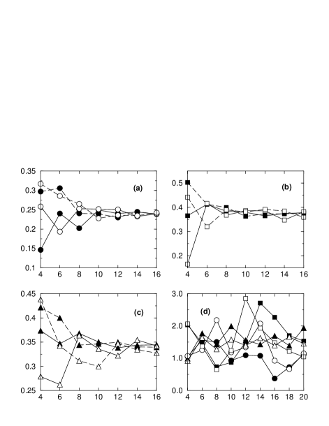
FIG. 3.: Nearest-neighbor spin correlations $S_{\alpha\beta}$ for wave functions with different boundary conditions on tori $L\times L$ as a function of the system size $L$. All wave functions have $\Delta_{0}=0.55$. (a): D1 wave function with $t^{\prime}=1.0$, $\mu=0.696$. (b): D2 wave function with $t^{\prime}=0.5$, $\mu=0.794$. (c): DD wave function with $D_{xy}=1.0$. In plots (a)–(c): solid symbols, solid lines correspond to $S_{+-}$; solid symbols, dashed lines — to $S_{-+}$; empty symbols, solid lines — to $S_{++}$; empty symbols, dashed lines — to $S_{--}$. (d): the spread of local correlations $\Delta S$ as a function of the system size $L$. Solid circles: D1 wave function, $t^{\prime}=1.0$, $\mu=0.696$. Empty circles: D1 wave function, $t^{\prime}=1.2$, $\mu=0.744$. Solid squares: D2 wave function, $t^{\prime}=0.5$, $\mu=0.794$. Empty squares: D2 wave function, $t^{\prime}=0.6$, $\mu=0.909$. Solid triangles: DD wave function, $D_{xy}=1.0$. Empty triangles: DD wave function, $D_{xy}=1.2$. In all plots, the error bars are smaller than the symbol size, except for the rightmost points in plot (d) where the error bars are of the order of the symbol size.

The first test for the topological order is the overlap of the two wave functions on a torus projected from the mean-field states with different boundary conditions. Note that when nodes in the mean-field excitation spectrum fall on points of the momentum lattice, the wave function becomes ill-defined. For our choice of lattice on the tori, this happens for the NND state where the nodes are fixed at ($\pm{\pi\over 2}$,$\pm{\pi\over 2}$) points. Therefore, not all four topological sectors are realized for the NND state (for our choice of the lattice placement). However, the sectors $+-$ and $-+$ are well-defined for any $L\times L$ torus, and we take the overlap between these two wave functions as the first check of the topological order. Alternatively, this overlap may be viewed as the overlap of the wave function with its reflection with respect to the $x$–$y$ diagonal.

We have calculated this overlap with the use of the variational Monte Carlo procedure[13]. The results for the NND wave function and for its three modifications D1, D2, and DD, are presented in Fig. 2a. In all cases, we take $\Delta_{0}=0.55$; for D1 wave functions we take $t^{\prime}=0.5$ ($\mu=0.417$) and $t^{\prime}=1.0$ ($\mu=0.696$); for D2 wave functions we take $t^{\prime}=0.3$ ($\mu=0.509$) and $t^{\prime}=0.5$ ($\mu=0.794$); for DD wave functions we take $D_{xy}=0.4$ and $D_{xy}=1.0$. We see that the overlap for the NND wave function saturates at large system size (which implies the absence of topological order), while for the three other wave functions it decreases to zero with increasing system size. This is the first signature of the topological order in those wave functions. As a side remark, we mention that if we force $\mu=0$ in the D2 wave function, the projected wave function has no topological order (the overlap saturates at large $L$), but such a wave function violates the mean-field-density constraint (26), and we do not discuss it here.

For the wave functions deep in the “topologically ordered” phase, we can also verify the orthogonality of all the four topological sectors $++$, $+-$, $-+$, and $--$. The four corresponding overlaps are plotted for each of the wave functions D1, D2, and DD in Fig. 2b–d. All the overlaps for these wave functions decrease to zero with increasing system size, which indicates orthogonality of the four sectors.

The second test for the topologically ordered state is the equality of local expectation values between different topological sectors (condition (ii) of Section III). We verify this condition for the nearest-neighbor spin-spin correlations. In the four topological sectors on the torus, there are four different nearest-neighbor correlators:

$$S_{+-} \equiv -\langle{+-}|\sigma^{z}_{i}\sigma^{z}_{i+\hat{\bf x}}|{+-}\rangle,$$ (42)

$$S_{-+} \equiv -\langle{+-}|\sigma^{z}_{i}\sigma^{z}_{i+\hat{\bf y}}|{+-}\rangle,$$ (43)

$$S_{++} \equiv -\langle{++}|\sigma^{z}_{i}\sigma^{z}_{j}|{++}\rangle,$$ (44)

$$S_{--} \equiv -\langle{--}|\sigma^{z}_{i}\sigma^{z}_{j}|{--}\rangle.$$ (45)

In a topologically ordered state, the difference between these four quantities must rapidly decay with increasing system size. We compute these correlators numerically for the same three wave functions used before in the overlap computations. The results are presented in Fig. 3a–c demonstrating that the four correlations indeed converge to a single value in large systems. This supports the contention that the distinction between the states is in global properties and not in local ones.

To quantify the rate of this convergence, we consider the mean square deviation of the four quantities $S_{+-}$, $S_{-+}$, $S_{++}$, and $S_{--}$. In Fig. 3d, we plot this mean square deviation multiplied by the number of lattice sites

$$\Delta S\equiv L^{2}\left[{\sum_{\alpha\beta}S_{\alpha\beta}^{2}\over 4}-\left({\sum_{\alpha\beta}S_{\alpha\beta}\over 4}\right)^{2}\right]^{1/2}$$ (46)

as a function of system size. The finite-size effects are very strong because of the nodes in the spectrum. To clarify the size dependence of $\Delta S$, we take one more wave function in each of the three classes D1, D2, DD, with slightly different variational parameters (in addition to the wave functions considered previously). The data in Fig. 3d indicate that $\Delta S$ remains approximately independent of system size. This corresponds to the difference in local correlations $S_{\alpha\beta}$ decaying as $L^{-2}$ with system size.

This slow convergence of correlations among different topological sectors can be explained already at the mean-field level from the nodal singularities in the spectrum. At the nodal points, the vector $(u_{\vec{k}},v_{\vec{k}})$ has a strong singularity: as the wave vector $\vec{k}$ goes around the nodal point, the vector $(u,v)$ rotates by half turn in the plane. This singularity translates into the $L^{-2}$ dependence of local correlations on the boundary conditions (changing the boundary conditions amounts to shifting the lattice of vectors $\vec{k}$). From our numerical results we see that this rate of convergence is preserved by the projection. This may serve as an indication that in the $Z_{2}$ states the projection preserves the nodal spinons, as suggested by Wen[23]. This $L^{-2}$ law applies to the general case of local correlations. The energy expectation value is a very special local correlation which has a weaker singularity at the nodal point. At the mean-field level, the energy splitting between different topological sectors can be found to be $L^{-3}$ (per site). This translates into the splitting in total energy decaying as $L^{-1}$. We expect that this asymptotic law also holds after the projection. To verify this numerically, one needs to compute the expectation values of the actual “energy”, which is a correlation function optimized for a particular Hamiltonian by adjusting the variational parameters. In this paper we do not identify spin Hamiltonians for which our wave functions are optimal, and thus are not able to verify our expectation for the energy splitting. Note that the $L^{-1}$ convergence in energy also means convergence of the energy of an individual vison, i.e., deconfinement of visons which is necessary for the topological order.

We have also tested all the above classes of wave functions for the valence-bond crystal (“spin-Peierls”) ordering[27]. We have computed the correlations of the $z$-component of the singlet order parameter $\langle S_{z}(i)S_{z}(i+{\bf x})S_{z}(j)S_{z}(j+{\bf x})\rangle$ in systems as large as 18$\times$18. We find this correlation function rapidly decaying with increasing the distance $|i-j|$. The decay is slowest for the D2 wave function for which it appears to be close to $R^{-2}$ (for the $t^{\prime}=0.5$, $\mu=0.794$ wave function) or faster (for the $t^{\prime}=0.6$, $\mu=0.909$ wave function). For D1 and DD wave functions the decay of such correlations is much stronger than in the D2 wave function, which indicates the absence of the valence-bond ordering. Note that the D2 wave functions for the values of parameters considered in this paper exhibit a relatively large correlation length for the overlaps between topological sectors (see Fig. 2c for the data on the $t^{\prime}=0.5$, $\mu=0.794$ wave function). Therefore one may expect that correlation functions have different behavior at larger and smaller length scale, and that our computations in relatively small systems are therefore not completely reliable for determining the correct long-distance behavior of the correlations. A more detailed analysis of the valence-bond crystal ordering and of its interplay with the topological order is left for future study.

V Conclusion

In this paper, we have formulated conditions for the presence of topological order in RVB systems and have verified them for several specific examples of Gutzwiller-projected wave functions. Our results suggest that appropriate Gutzwiller-projected wave functions may represent ground states of fractionalized phases of spin systems.

This work is only the first step towards describing the topologically ordered RVB states. For a better understanding of the properties of the topological order, a more extensive quantitative study is needed. It should include an analysis of correlation lengths involved in the conditions (i) and (ii) for the topological order (in particular, on cylinders/tori with different aspect ratios). Variational wave functions may provide a useful tool for studying quantum phase transitions between states with and without topological order. An extremely interesting question in this respect is the possibility of the coexistence of the topological order simultaneously with the antiferromagnetic Neel order or with the valence-bond crystal order. Such a coexistence of a topological and a conventional ordering may be tested by projecting appropriate superconducting states with the spin or translational symmetry broken before projection.

Of course, the study of the variational wave functions have physical implications only when the Hamiltonians are identified for which those wave functions are good trial states. Our test for the topological order may provide a guidance in the search for microscopic spin Hamiltonians that exhibit fractionalized ground states.

We thank P. A. Lee, X.-G. Wen, A. Ioselevich, M. Feigelman, L. Ioffe, G. Blatter, M. P. A. Fisher, and O. Motrunich for useful discussions. We are grateful to A. Paramekanti, M. Randeria, and N. Trivedi for sharing their unpublished results and for several useful conversations. This work was supported by MRSEC program of the National Science Foundation under grant DMR-9808941 and by the Swiss National Foundation.

REFERENCES

- [1] P. W. Anderson, Science 235, 1196 (1987).
- [2] R. Coldea, D. A. Tennant, A. M. Tsvelik, and Z. Tylczynski, Phys. Rev. Lett. 86, 1335 (2001); G. Misguich et al, Phys. Rev. B 60, 1064 (1999); W. LiMing et al, Phys. Rev. B 62, 6372 (2000); S. Sachdev, Phys. Rev. B45, 12377 (1992); C. H. Chung, J. B. Marston, and R. H. McKenzie, J. Phys. C 13, 5159 (2001); C. H. Chung, J. B. Marston, and S. Sachdev, Phys. Rev. B 64, 134407 (2001); R. Moessner and S. L. Sondhi, Phys. Rev. Lett. 86, 1881 (2001); L. Balents, M. P. A. Fisher, and S. M. Girvin, cond-mat/0110005.
- [3] N. Read and S. Sachdev, Phys. Rev. Lett. 66, 1773 (1991); S. Sachdev and N. Read, Int. J. Mod. Phys. B 5, 219 (1991).
- [4] X. G. Wen, Phys. Rev. B 44, 2664 (1991).
- [5] C. Mudry and E. Fradkin, Phys. Rev. B49, 5200 (1994).
- [6] L. Balents, M. P. A. Fisher, and C. Nayak, Phys. Rev. B 60, 1654 (1999); ibid. 61, 6307 (2000).
- [7] T. Senthil and M. P. A. Fisher, Phys. Rev. B 62, 7850 (2000).
- [8] T. Senthil and O. Motrunich, cond-mat/0201320.
- [9] T. Senthil and M. P. A. Fisher, Phys. Rev. B 63, 134521 (2001).
- [10] X. G. Wen, Int. J. Mod. Phys. B 4, 239 (1990).
- [11] M. C. Gutzwiller, Phys. Rev. Lett. 10, 159 (1963); Phys. Rev. A 134, 1726 (1965).
- [12] H. Yokoyama and H. Shiba, J. Phys. Soc. Jpn. 57, 2482 (1988); H. Yokoyama and M. Ogata, J. Phys. Soc. Jpn. 65, 3615 (1996).
- [13] C. Gros, Phys. Rev. B 38 (1988), 931; Ann. Phys. 189, 53 (1989).
- [14] D. A. Ivanov, P. A. Lee, and X.-G. Wen, Phys. Rev. Lett. 84, 3958 (2000).
- [15] A. Paramekanti et. al., Phys. Rev. Lett., 87, 217002 (2001).
- [16] D. A. Bonn et.al, Nature 414, 887 (2001).
- [17] J. C. Wynn et.al, Phys. Rev. Lett. 87, 197002 (2001).
- [18] L. Capriotti, F. Becca, A. Parola, and S. Sorella, cond-mat/0107204.
- [19] N. Read and B. Chakraborty, Phys. Rev. B40, 7133 (1989). See also Ref. [21].
- [20] D. S. Rokhsar and S. A. Kivelson, Phys. Rev. lett. 61, 2376 (1988).
- [21] N. Bonesteel, Phys. Rev. B40, 8954 (1989).
- [22] We are grateful to X.G. Wen for emphasizing this to us.
- [23] X. G. Wen, cond-mat/0107071.
- [24] D. V. Dmitriev, V. Ya. Krivnov, V. N. Likhachev, and A. A. Ovchinnikov, Fiz. Tv. Tela. 38, 397 (1996). [Phys. Solid State 38, 219 (1996)]
- [25] F. C. Zhang, C. Gros, T. M. Rice, and H. Shiba, Supercond. Sci. Technol. 1, 36 (1988).
- [26] X.-G. Wen and P. A. Lee, Phys. Rev. Lett. 76, 503 (1996).
- [27] E. Fradkin, Field Theories of Condensed Matter Systems (Addison–Wesley, Redwood City, CA, 1991).