Explicit finite-difference and direct-simulation-MonteCarlo method for the dynamics of mixed Bose-condensate and cold-atom clouds

Abstract

We present a new numerical method for studying the dynamics of quantum fluids composed of a Bose-Einstein condensate and a cloud of bosonic or fermionic atoms in a mean-field approximation. It combines an explicit time-marching algorithm, previously developed for Bose-Einstein condensates in a harmonic or optical-lattice potential, with a particle-in-cell MonteCarlo approach to the equation of motion for the one-body Wigner distribution function in the cold-atom cloud. The method is tested against known analytical results on the free expansion of a fermion cloud from a cylindrical harmonic trap and is validated by examining how the expansion of the fermionic cloud is affected by the simultaneous expansion of a condensate. We then present wholly original calculations on a condensate and a thermal cloud inside a harmonic well and a superposed optical lattice, by addressing the free expansion of the two components and their oscillations under an applied harmonic force. These results are discussed in the light of relevant theories and experiments.

I Introduction

The physics of ultracold atomic vapours under magnetic or optical confinement has been a continuing and ever expanding focus of interest since the realization of Bose-Einstein condensation [1]. Following characterizations of the basic thermodynamic and dynamical properties of condensates [2], a number of experiments have been addressed to investigations of their phase coherence and superfluidity [3], to the study of non-linear effects and special spectroscopic features  [4], and to the observation of vortices [5]. Parallel efforts are being made in the study of gases of fermionic atoms [6] and of boson-fermion mixtures [7], with the ultimate aim of realizing novel superfluids.

Theoretical studies of the dynamics of these systems, involving the analytical solution of approximate models have very often been successful in explaining or predicting such novel phenomena. However, the interplay of different species or the thermal fluctuations of a condensate are not easily handled by analytical methods. The validity of the approximations may be limited to the extreme collisionless or hydrodynamic regimes, the confinement of the sample being treated within a local-density approach. Thus, while the equations governing these dilute systems remain simple, their numerical solution can be helpful for investigating more complex dynamical problems where an intermediate regime is met or a cold-atom cloud accompanies the condensate.

The atomic interactions in a highly dilute Bose gas at very low temperatures, as is relevant for current experiments, are described by a contact pseudopotential accounting for $s$-wave scattering in binary atom-atom elastic collisions. A condensate is then treated within a mean-field approach by solving the stationary or the time-dependent Gross-Pitaevskii equation (GPE). Several types of numerical approaches have been developed: eigenvalue solvers[8], variational solvers[9], or explicit solvers [10] for the ground state, and implicit [11] or explicit [12] time-marching schemes for the dynamics.

Methods for studying the dynamics of an isolated cloud of ultracold (bosonic or fermionic) atoms are also well developed. One needs to solve the Vlasov-Landau equation of motion (VLE) for the Wigner distribution function. Various numerical techniques have been used for this purpose, which are based either on an ergodic assumption [13] or on the inclusion of statistical noise [14], or else use a direct simulation MonteCarlo (DSMC) approach borrowed from the methods of molecular dynamics [15, 16, 17].

The general theoretical background is provided by the book of Kadanoff and Baym [18]. These authors developed a Green’s function approach to transport phenomena, which extends the Boltzmann equation to strongly interacting quantum fluids and allows for progressively improved self-consistent approximations. This formalism was extended to a homogeneous Bose-condensed gas at finite temperature by Kane and Kadanoff [19], within a Beliaev approximation including interactions up to second order. More recently, these methods have been adapted to the theory of transport phenomena in a confined Bose gas within the Hartree-Fock-Bogoliubov approximation [20, 21, 22], dealing with a Bose-Einstein condensate accompanied by its thermal cloud. Jackson and Adams [23] have proposed to combine the GPE with a quantum version of the DSMC to numerically evaluate the dynamics of such a fluid. Numerical studies based on a generalized GPE combined with a semiclassical kinetic equation, and including collisions between the condensate and the thermal cloud, are also becoming avaible for dynamical properties of a trapped Bose-condensed gas at finite temperature  [24].

In the present work we proceed along the path traced by Jackson and Adams [23]. We propose a different approach to the solution of the GPE and a different method for preparing the initial equilibrium state, which would be immediately applicable to a multi-component cold-atom cloud. The method is applied to two classes of dynamical problems: the first concerns the ballistic expansion of a fermion cloud and the role played by the presence of a condensate, while the second concerns a Bose-condensed gas in a periodic optical-lattice potential at finite temperature.

After introducing in Sec. II the model for both the equilibrium state and the dynamical evolution of the fluid, we describe in Sec. III the numerical methods that we have used to consistently solve the GPE for the condensate and the VLE for the Wigner distribution function of the cloud. The procedure followed in the actual computations is also outlined in Sec. III, with due emphasis on the preparation of the initial equilibrium state. The physical applications that we have carried out are presented and discussed in Sec. IV. A discussion of computational aspects in Sec. V and some final remarks in Sec. VI conclude the paper.

II The model: a review of the main concepts

A Transport in a normal quantum fluid

In the original formulation by Kadanoff and Baym (KB), the problem of transport in a quantum fluids in the normal state is tackled by deriving an analogue of the Boltzmann equation for the Wigner distribution function $f({\bf p},{\bf r},t)$ from the microscopic equations of motion for the non-equilibrium density matrix $\rho({\bf r}_{1},t_{1};{\bf r}_{1^{\prime}}t_{1^{\prime}})\equiv<\psi^{\dagger}_{\cal U}({\bf r}_{1},t_{1})\psi_{\cal U}({\bf r}_{1^{\prime}},t_{1^{\prime}})>$, which is defined through the particle creation and destruction operators $\psi_{\cal U}^{(\dagger)}$ in the presence of an external, slowly varying disturbance ${\cal U}({\bf r},t)$. Namely,

$$f({\bf p},{\bf r},t)=\int d{\bf x}\exp(-i{\bf p}\cdot{\bf x})<\psi^{\dagger}_{\cal U}({\bf r}+{\bf x}/2,0)\psi_{\cal U}({\bf r}-{\bf x}/2,t)>\;$$ (1)

where ${\bf r}=({\bf r}_{1}+{\bf r}_{1^{\prime}})/2$ and ${\bf x}={\bf r}_{1}-{\bf r}_{1^{\prime}}$ are the center-of-mass and the relative coordinate of the two particles. The moments of the Wigner function yield observables such as the particle density $n({\bf r},t)=(2\pi)^{-3}\int d{\bf p}f({\bf p},{\bf r},t)$ and the current density ${\bf j}({\bf r},t)=(2\pi)^{-3}\int d{\bf p}\,({\bf p}/m)\,f({\bf p},{\bf r},t)$.

Contact with the Boltzmann transport equation is made by performing gradient expansions. As in the conventional Boltzmann-equation approach, the validity of the KB formulation is limited to slowly varying perturbations. On the other hand, the advantage of the KB formulation is that higher-order correlations enter the equation of motion for the density matrix in an explicit manner, and therefore systematically improved approximations which are consistent with the conservation laws are accessible. Examples of such treatments of the correlation term are the Hartree approximation and the Born-collision approximation. In the former case the collisionless Boltzmann equation is recovered, while in the latter the collisional Boltzmann equation is extended to non-dilute systems by including the effect of the external potential on the motion of the particles between collisions.

B Extension to coupled condensate-noncondensate dynamics

The extension of the KB treatment to gases including a Bose-condensed component has been made by Kane and Kadanoff [19] and further developed by Griffin and coworkers [20, 21] and also by Wachter et al. [22] through a different derivation. The presence of two components and the appearence of off-diagonal elements in the density matrix (the so-called anomalous densities) below the Bose-Einstein condensation temperature requires the introduction of three Wigner distribution functions: $f_{c}({\bf p},{\bf r},t)$ for the condensate component described by $<\psi^{(\dagger)}_{\cal U}>$ and involving $|<\psi^{\dagger}_{\cal U}>|^{2}$, ${f_{b}}({\bf p},{\bf r},t)$ for the noncondensate described by the fluctuations operators $\tilde{\psi}^{(\dagger)}_{\cal U}\equiv\psi^{(\dagger)}_{\cal U}-<\psi^{(\dagger)}_{\cal U}>$ and involving $<\tilde{\psi}^{\dagger}_{\cal U}\tilde{\psi}_{\cal U}>$, and ${f}_{m}({\bf p},{\bf r},t)$ for the anomalous part involving $<\tilde{\psi}_{\cal U}\tilde{\psi}_{\cal U}>$ and its Hermitean conjugate.

We thus have to deal with the density of condensate $n_{c}({\bf r},t)=(2\pi)^{-3}\int d{\bf p}\,f_{c}({\bf p},{\bf r},t)$, the density of noncondensate $n_{b}({\bf r},t)=(2\pi)^{-3}\int d{\bf p}\,{f_{b}}({\bf p},{\bf r},t)$, and the anomalous density ${m}({\bf r},t)=(2\pi)^{-3}\int d{\bf p}\,{f}_{m}({\bf p},{\bf r},t)$. Analogous expressions holds for the current densities.

As to the consistency of the approximations with the conservation laws, the same general remarks as for normal systems apply. However, the appearence of the condensate introduces an additional principle of gauge invariance, leading to the requirement that the excitation spectrum to be gapless [25]. It is well known [20, 25] that approximations capable of simultaneously accommodating the conservation laws and the gaplessness condition are hardly available, so that a choice has to be made depending on the specific conditions of density and temperature of the system.

In the regime that we address in the present work the anomalous densities can be neglected, resulting in the gapless Hartree-Fock-Bogoliubov-Popov approximation [20]. Thus, the equation of motion for the condensate wavefunction $\Phi({\bf r},t)\equiv<\psi^{\dagger}_{\cal U}({\bf r},t)>$ is

$$i\hbar\frac{\partial\Phi({\bf r},t)}{\partial t}=\left[-\frac{\hbar^{2}}{2m}\hbox{\rm\boldmath{$\nabla$}}^{2}+V^{eff}_{c,b}({\bf r},t)\right]\Phi({\bf r},t)$$ (2)

and is coupled to the collisionless Vlasov equation for the noncondensate Wigner function ${f}_{b}({\bf p},{\bf r},t)$,

$$\frac{\partial{f}_{b}({\bf p},{\bf r},t)}{\partial t}+\frac{{\bf p}}{m}\cdot\hbox{\rm\boldmath{$\nabla_{\bf r}$}}{f}_{b}({\bf p},{\bf r},t)-\hbox{\rm\boldmath{$\nabla_{\bf r}$}}V^{eff}_{b}({\bf r},t)\cdot\hbox{\rm\boldmath{$\nabla$}}_{\bf p}{f}_{b}({\bf p},{\bf r},t)=0\;.$$ (3)

The mean-field potentials in Eqs. (2) and (3) are

$$V^{eff}_{c,b}({\bf r},t)=V^{ext}_{b}({\bf r})+{\cal U}({\bf r},t)+U_{g}[n_{c}({\bf r},t)+2{n}_{b}({\bf r},t)]\;$$ (4)

and

$$V^{eff}_{b}({\bf r},t)=V^{ext}_{b}({\bf r})+{\cal U}({\bf r},t)+2U_{g}[n_{c}({\bf r},t)+{n}_{b}({\bf r},t)]\;,$$ (5)

including the time-dependent driving potential ${\cal U}({\bf r},t)$ and an axially symmetric confining potential given for a harmonic trap by $V^{ext}_{b}({\bf r})=m_{b}\omega_{b}^{2}(r_{\perp}^{2}+\epsilon_{b}^{2}z^{2})/2$. In Eqs. (4) and (5), $n_{c}({\bf r},t)=|\Phi({\bf r},t)|^{2}$ and $U_{g}=4\pi\hbar^{2}a_{bb}/m_{b}$ is the boson-boson interaction parameter in terms of the $s$-wave scattering length $a_{bb}$ and of the boson mass $m_{b}$.

Once the algorithm to solve Eqs. (2) and (3) is implemented, it is easily extended to a mixture of condensed bosons and a fermionic cloud in the collisionless regime. In this case, the effective mean-field potentials become

$$V^{eff}_{c,f}({\bf r},t)=V^{ext}_{b}({\bf r})+{\cal U}({\bf r},t)+U_{g}n_{c}({\bf r},t)+U_{f}n_{f}({\bf r},t)$$ (6)

and

$$V^{eff}_{f}({\bf r},t)=V^{ext}_{f}({\bf r})+{\cal U}_{f}({\bf r},t)+U_{f}n_{c}({\bf r},t)\;.$$ (7)

Here, $V^{ext}_{f}({\bf r})=m_{f}\omega_{f}^{2}(r_{\perp}^{2}+\epsilon_{f}^{2}z^{2})/2$ and ${\cal U}_{f}({\bf r},t)$ are the external trapping and driving potentials acting on the fermions and $U_{f}=2\pi\hbar^{2}a_{bf}/m_{r}$ is the boson-fermion coupling constant with $a_{bf}$ the boson-fermion $s$-wave scattering length and $m_{r}=m_{b}m_{f}/(m_{b}+m_{f})$, $m_{f}$ being the fermion atomic mass. Notice that fermion-fermion collisions in the $s$-wave channel are effectively suppressed by the Pauli principle in a dilute gas of spin-polarized fermions, as is relevant to current experiments on boson-fermion mixtures.

C Validity of the model

To summarize, Eqs. (2) and (3) describe the coupled dynamics of a Bose-Einstein condensate and a bosonic or fermionic cold-atom cloud. In the former case the potentials $V^{eff}_{c,b}$ and $V^{eff}_{b}$ are used, and in the latter these are replaced by $V^{eff}_{c,f}$ and $V^{eff}_{f}$. The range of validity of this approach is in principle limited to: (i) slowly varying space- and time-dependent external potentials, which allows a low-order gradient expansion of the equations of motion for the one-body density matrix; (ii) a collisionless regime, which allows expansion of the self-energies to first order in the strength of the atomic interactions; and (iii) not too low temperature, so that the anomalous averages can be neglected.

We implement below a numerical method to solve Eqs. (2) and (3) and test it against dynamical behaviors in a one-component fermionic cloud and in clouds of either fermions or thermal bosons accompanied by a condensate. Of course, the role of the statistics enters at this level only from the initial distribution of the particles in phase space. We thus turn to discuss the equations that we use to determine the initial conditions for the subsequent time evolution.

D Semiclassical description of the equilibrium state

Before proceeding to present the algorithm for our dynamical simulations we briefly recall the basic steps that we take in preparing the initial state of the gas in thermodynamic equilibrium and in evaluating the corresponding densities of the condensate and of the fermionic or bosonic cloud. We refer the reader to Ref. [26, 27] for the details of the theory and for a discussion of the excellent agreement that it yelds with thermodynamic data on Bose-Einstein condensed gases, under conditions of temperature and dilution that will be verified in the calculations reported in Section IV below.

The equilibrium condensate density is calculated within the Thomas-Fermi approximation, which amounts to neglecting the kinetic energy term in the GPE. Its validity is ensured whenever the average mean-field energy $U_{g}n_{c}$ is much larger than the typical confining energy. In the case of harmonic confinement the condition $N_{c}a_{bb}/a_{ho}\gg 1$ is required, where $N_{c}$ is the number of atoms in the condensate, $a_{ho}=(\hbar/m_{b}\overline{\omega}_{b})^{1/2}$ is the harmonic oscillator length and $\overline{\omega}_{b}=\omega_{b}\epsilon^{1/3}$ is the geometric average of the trap frequencies. The equilibrium density profile of the condensate is given by

$$n_{c}({\bf r})=\frac{1}{U_{g}}\,\left[\mu_{b}-V^{ext}_{b}({\bf r})-k_{b,f}n_{b,f}({\bf r})\right]\,\theta(\mu_{b}-V^{ext}_{b}({\bf r})-k_{b,f}n_{b,f}({\bf r}))$$ (8)

where $k_{b}=2U_{g}$, $k_{f}=U_{f}$ and $\mu_{b}$ is the chemical potential for the bosons.

For the equilibrium cloud density of bosons or fermions we adopt the semiclassical Hartree-Fock scheme [26]. This choice is justified as long as the gas is in a very dilute regime, a condition which is usually met in current experiments. In this approximation we have

$$n_{b,f}({\bf r})=\int\frac{{\rm d}{\bf p}}{(2\pi)^{3}}\left\{\exp{\left[\frac{1}{k_{B}T}\left(\frac{p^{2}}{2m_{b,f}}+V^{eff}_{b,f}({\bf r})-\mu_{b,f}\right)\right]}\mp 1\right\}^{-1},$$ (9)

with $V^{eff}_{b}({\bf r})$ and $V^{eff}_{f}({\bf r})$ determined by the confining potentials supplemented by static mean-field interaction term as in Eqs. (5) or (7).

The chemical potentials $\mu_{b}$ and $\mu_{f}$ are determined from the total numbers of bosons and fermions. In the case of a bosonic thermal cloud, $\mu_{b}$ is fixed by the relation

$$N_{b}=\int{\rm d}{\bf r}\left[n_{c}({\bf r})+n_{b}({\bf r})\right]\,.$$ (10)

For a fermionic cloud the chemical potential is determined from the total number of fermions,

$$N_{f}=\int{\rm d}{\bf r}\,N_{f}({\bf r})\,.$$ (11)

These equations complete the self-consistent closure of the model in the initial equilibrium state.

III The numerical method

In this section we present the numerical procedure that we have used to solve the system of Vlasov-Landau and Gross-Pitaevskii equations. Since most experimental setups are invariant under rotation in the azimuthal plane, we use cylindrical coordinates $\{r,z\}$. The wavefunction $\Phi$ is discretized on a two-dimensional grid of $N_{r}\times N_{z}$ points, which are uniformly distributed in a box of sizes $r_{max}\times 2z_{max}$: that is, $\Phi_{jk}\equiv\Phi(r_{j},z_{k})$ with

$$\left\{\begin{array}[]{lr}r_{j}=(j-1)\Delta r&\;\;\;(j=1,\dots,N_{r})\\ z_{k}=-z_{max}+(k-1)\Delta z&\;\;\;(k=1,\dots,N_{z})\\ \end{array}\right.$$ (12)

$\Delta r$ and $\Delta z$ being the steps in the two space variables. The particle distributions are discretized by means of a set of $P$ computational particles,

$$f({\bf p},{\bf r},t)\rightarrow f_{P}({\bf p},{\bf r},t)\equiv\sum_{i=1}^{P}\delta({\bf r}-{\bf r}_{i}(t))\delta({\bf p}-{\bf p}_{i}(t))$$ (13)

where the $6P$ phase-space coordinates ${\bf r}_{i}(t)$ and ${\bf p}_{i}(t)$ represent the actual numerical unknowns entering the VLE. They obey Newton’s equations,

$$\left\{\begin{array}[]{ll}\dfrac{d{\bf r}_{i}}{dt}={\bf p}_{i}/m\\ \dfrac{d{\bf p}_{i}}{dt}={\bf F}_{i}\end{array}\right.$$ (14)

where ${\bf F}_{i}$ collects all forces acting on the $i$-th computational particle. As a result, at each time step we have to solve for $N_{G}=N_{r}N_{z}$ grid unknowns coupled to $6P$ discrete particle coordinates. In order to keep the systematic signal reasonably above the noise level, each grid cell contains of the order of $10-100$ computational particles. As a result, $P\sim 10N_{G}-100N_{G}$.

A Propagation of the Gross-Pitaevskii equation

The GPE is advanced in time by an explicit finite-difference method based on a non-staggered variant of the Visscher method [28]. The full details are given in original papers [12, 10] and here we shall just review the main ingredients of the algorithm. The basic idea is to advance the real and imaginary parts of the wavefunction, say $A$ and $B$, in alternating steps as follows:

$$\left\{\begin{array}[]{ll}A_{jk}^{n+1}-A_{jk}^{n-1}=-2[K_{jk}(B)+V_{jk}^{n}(B)]\Delta t\\ B_{jk}^{n+1}-B_{jk}^{n-1}=2[K_{jk}(A)+V_{jk}^{n}(A)]\Delta t\end{array}\right.$$ (15)

where $n=1,\dots,N_{T}$ labels the discrete time sequence $t_{n}=n\Delta t$. The scheme is initiated as follows. The initial conditions specify the values of $A$ and $B$ at $n=0$ and subsequently a first-order Euler step provides their values at $n=1$. With these values available, all later steps $n=2,3,\dots,N_{T}$ are taken by using the above set of equations.

In Eq. (15) $K_{jk}$ is the kinetic energy operator,

$$K_{jk}(\Phi)=-\frac{\hbar^{2}}{2m}[\frac{\Phi_{j-1,k}}{{\Delta r}^{2}}+\frac{\Phi_{j+1,k}}{{\Delta r}^{2}}+\frac{\Phi_{j,k-1}}{{\Delta z}^{2}}+\frac{\Phi_{j,k+1}}{{\Delta z}^{2}}-2(\frac{1}{{\Delta r}^{2}}+\frac{1}{{\Delta z}^{2}})\;\Phi_{j,k}]$$ (16)

and

$$V_{jk}(\Phi)=V^{eff}(r_{j},z_{k};n_{jk})\Phi_{jk}$$ (17)

is the potential energy operator, including both external and self-consistent interaction terms. The self-consistent potential requires the specification of the particle density $n_{jk}$ at each node of the spatial grid. This is obtained by convoluting the discrete particle distribution,

$$n_{jk}(t)=\sum_{i\in C_{jk}}W_{jk,i}f_{i}(t)$$ (18)

where $C_{jk}$ is the grid cell centered in $r_{j+1/2}=(r_{j}+r_{j+1})/2$, and $z_{k+1/2}=(z_{k}+z_{k+1})/2$, while $f_{i}=1$ if the particle belongs to $C_{jk}$ and $f_{i}=0$ otherwise. The factor $W_{jk,i}$ weights the contribution of particle $i$ to the density at the grid-point $(r_{j},z_{k})$.

We adopt a bilinear ”cloud-in-cell” (CIC) interpolator (see fig. 1a), which yields the scattering (particle-to-grid) rule [29]

$$W_{jk,i}=e_{i}(r_{j})e_{i}(z_{k})\;\;\;(j=j_{i},j_{i}+1,\;\;\;k=k_{i},k_{i}+1).$$ (19)

Here $(j_{i},k_{i})$ identifies the lower-left corner of the grid cell to which the $i$-th particle belongs. In Eq. (19) $e_{i}(r)$ and $e_{i}(z)$ are one-dimensional piecewise linear splines centered on the discrete particle position $(r_{i},z_{i})$,

$$e_{i}(r)=\left\{\begin{array}[]{r}1+\dfrac{(r-r_{i})}{\Delta r}\qquad\;\;\;(r_{i}-\Delta r<r<r_{i})\\ 1-\dfrac{(r-r_{i})}{\Delta r}\qquad\;\;\;(r_{i}<r<r_{i}+\Delta r)\end{array}\right.$$ (20)

and similarly for $e_{i}(z)$.

B Propagating the Vlasov-Landau equation

The VLE is advanced in time by a standard Particle-in-Cell (PIC) method [29]. In a modified Verlet time-marching scheme, we obtain the following set of discrete algebraic equations:

$$\left\{\begin{array}[]{lll}r_{i}(t+\Delta t)=r_{i}(t)+v_{ri}(t)\Delta t+a_{ri}(t){\Delta t}^{2}/2\\ (r_{i}\theta_{i})(t+\Delta t)=(r_{i}\theta_{i})(t)+v_{\theta i}(t)\Delta t+a_{\theta i}(t){\Delta t}^{2}/2\\ z_{i}(t+\Delta t)=z_{i}(t)+v_{zi}(t)\Delta t+a_{zi}(t){\Delta t}^{2}/2\\ v_{ri}(t+\Delta t)=v_{ri}(t)+a_{ri}(t){\Delta t}\\ v_{\theta i}(t+\Delta t)=v_{\theta i}(t)+a_{\theta i}(t){\Delta t}\\ v_{zi}(t+\Delta t)=v_{zi}(t)+a_{zi}(t){\Delta t}\end{array}\right.$$ (21)

Here $a_{r},a_{\theta},a_{z}$ and $v_{r},v_{\theta},v_{z}$ are the three components of the acceleration and of the velocity along the $(r,\theta,z)$ coordinates. The advantage of the modified Verlet time marching is that fourth-order accuracy is preserved while synchronously keeping the coordinate and momentum degrees of freedom on the same sequence of discrete times.

The algorithm is standard except for the specification of the self-consistent coupling, namely the force due to the density gradients. In the first place, we form density gradients from auxiliary values of the density field $n_{j+1/2,k+1/2}$ at cell centers,

$$\left\{\begin{array}[]{ll}Gr_{ij}=[n_{j+1/2,k-1/2}-n_{j-1/2,k-1/2}+n_{j+1/2,k+1/2}-n_{j-1/2,k+1/2}]/(2\Delta r)\\ Gz_{ij}=[n_{j-1/2,k+1/2}-n_{j-1/2,k-1/2}+n_{j+1/2,k+1/2}-n_{j-1/2,k-1/2}]/(2\Delta z)\end{array}\right.$$ (22)

The azimuthal acceleration is zero in cylindrical symmmetry. Next, the grid-forces are evaluated on the discrete particle locations, this being the inverse of the scattering operation discussed in the previous section (see fig. 1b). The grid-to-particle convolution is

$${\bf F}_{i}=\sum_{s=0}^{1}W_{i,(j+s,k+s)}{\bf F}_{j+s,k+s}.$$ (23)

In order to avoid spurious self-forces we use again CIC-interpolation, which amounts to using the same weighting function as for the GPE in the grid-to-particle scattering rule,

$$W_{i,jk}=e_{j}(r_{i})e_{k}(z_{i}).$$ (24)

With the force/acceleration field transferred to the particle locations, everything is set to march the VLE in time.

C Boundary conditions

The conditions imposed on the wavefunction are (i) periodicity along the $z$ coordinate, (ii) symmetry (zero radial gradient) at $r=0$, and (iii) vanishing at the outer radial boundary $r=R$. For the discrete particle distribution we have again periodicity along $z$ and specular reflection at the outer radial boundary. Specular reflection means that a particle flying from, say, $r_{\alpha}<R$ to $r_{\beta}>R$ is replaced by a particle at $r=2R-r_{\beta}$ with inverted radial speed. Since the particle trajectories are tracked in a three-dimensional cylindrical coordinate frame, the $r=0$ axis requires no special treatment.

1 Time-step considerations

The GPE and the VLE are advanced on the same discrete time sequence. This maximizes simplicity, but implies that the time-step is controlled by the fastest process at work, which usually is the self-consistent potential acting upon the condensate wavefunction. Better efficiency can be achieved by sub-cycling the time-stepper, namely by advancing the slowest equation (say the VLE) only every $\Delta t_{VL}/\Delta t_{GP}$ steps, $\Delta t_{VL}$ and $\Delta t_{GP}$ being the largest time-steps allowed by the stability conditions on the two equations. The maximum time-step for the GPE solver is estimated from

$$\Delta t_{GP}(C_{1}\frac{\hbar}{m\delta^{2}}+C_{2}\hbar\dfrac{V_{M}}{\hbar})<1$$ (25)

where $\delta$ is a typical mesh size, $V_{M}$ is the maximum value of the potential and $C_{1}$ and $C_{2}$ are two coefficients $O(1)$ which depend on geometry and dimensionality. We note here the concurrent effects of quantum diffusion (kinetic energy) and scattering/absorption (potential energy).

The maximum time-step for the VLE solver is estimated from

$$\Delta t_{VL}\frac{v_{max}}{\delta}<1$$ (26)

where $v_{max}$ is the maximum speed in the velocity grid, of the order of the Fermi velocity for fermions and of the thermal velocity for bosons. Under ordinary conditions the kinetic energy contributions dominate over those from the potential energy, so that the condition for the GPE to be the time-limiting section of the code takes the form of a numerical “uncertainty principle”, $mv_{max}\delta>\hbar$. For the cases discussed in this work, this inequality is generally fulfilled within a factor ten, so that sub-cycling is not compulsory. The inclusion of collisional interactions would make it mandatory.

2 Radial singularity

A source of potential trouble is the singularity in $r=0$, which is known to affect all calculations in polar coordinates. To date, singular factors $1/r$ are regularized by a simple numerical cutoff $1/r\rightarrow 1/(r+r_{c})$ with $r_{c}\sim 0.001\Delta r$, with a check that the physical results are virtually insensitive to the specific value of $r_{c}$.

Another undesirable side-effect of the cylindrical geometry is the relative depletion of near-axis cells, which tend to host fewer particles just because of the $r\Delta r$ volumetric effect. On the other hand, this volumetric depletion is often more than compensated by the physical behavior of the radial density, which is generally largest at $r=0$. At any rate, the volumetric effect can be readily disposed of by moving to a non-uniform grid along the radial coordinate.

3 Statistical noise

Considerations of statistical accuracy require of the order of a few tens of particles per grid-point (or equivalently per grid-cell) in order to keep the noise-to-signal ratio below an acceptable threshold. A practical consequence of this statistical accuracy requirement is that the VLE part of the computational scheme should be designed in such a way as to evolve these tens of computational particles in approximately the same amount of CPU time that it takes the GPE solver to advance a single grid-point.

Another interesting consequence is that - at variance from ordinary situations in (classical) rarefied-gas dynamics - the number of computational particles in the simulation of Bose-Einstein condensates far exceeds the number of physical atoms, typically by a factor $10^{3}$ in our case. As a result, each single computer simulation performs de facto a built-in ensemble average over a set of about a thousand realizations.

D Procedure: preparing the initial state

The initial condition for the populations of bosons or fermions in the cold-atom cloud is prepared as follows. Particles are sampled from the probability distribution functions (pdf)

$$f_{b,f}=\frac{e^{-\eta}}{1\mp e^{-\eta}}$$ (27)

where $\eta\equiv\beta(\mu_{b,f}-V_{eff}+p^{2}/2m)$ with $\beta=1/k_{B}T$ the inverse temperature.

The initializiation procedure starts by assigning to each spatial cell centered about position ${\bf r}$ a corresponding amount of computational particles,

$$\Delta N({\bf r})=n_{b,f}({\bf r})\Delta V({\bf r})$$ (28)

where $\Delta V({\bf r})=2\pi r\Delta r\Delta z$ is the cell volume. These particles must be sampled in momentum space according to the pdf (27). Owing to the non-separability of the pdf, straightforward sampling based on exact inversion is ruled out and more general - but less efficient - accept/reject methods must be resorted to.

The particle momenta are sampled from the distribution function using the standard Box-Mueller algorithm in three dimensions for cylindrical coordinates[30],

$$\left\{\begin{array}[]{l}p_{\perp}=p_{max}r_{1}\\ \xi=2\pi r_{2}\\ p_{z}=p_{max}(2r_{3}-1)\\ \end{array}\right.$$ (29)

where $r_{1}$, $r_{2}$ and $r_{3}$ are sampled from a uniform distribution in the range $[0,1]$. The maximum momentum $p_{max}$ is taken to be of order $2p_{F}$ for cold fermions and of order $3m_{b}v_{th}$ for bosons, with $p_{F}=\hbar k_{f}$ being the Fermi momentum and $v_{th}$ the average thermal velocity. The particle momentum coordinates in the azimuthal plane are evaluated as

$$\left\{\begin{array}[]{lll}p_{r}&=&p_{\perp}sin\xi\\ p_{\theta}&=&p_{\perp}cos\xi.\\ \end{array}\right.$$ (30)

Finally, in order to avoid poor acceptance rates, the standard accept/reject test is performed by comparing the pdf with the maximum value $f_{max}({\bf r})$ that it can take in the cell at position ${\bf r}$, that is

$$I\!f\;f(p_{r},p_{\theta},p_{z};{\bf r})>r_{4}f_{max}({\bf r}):\;accept$$ (31)

$$Else:\;reject$$ (32)

where $r_{4}$ is a random number uniformly distributed in $[0,1]$.

IV Physical applications

A Expansion of cold fermions

As a first test of the dynamical algorithm, we consider the expansion of a cloud of cold fermions after release of the harmonic trap. The neglect of the collisional integrals is a reliable approximation in this context, since as already remarked the $s$-wave scattering between spin-polarized fermions is suppressed by the Pauli principle.

This problem has been analytically solved in Ref. [31] under the assumption of ballistic expansion. The time-evolution of the mean square radii is found to be

$$<r_{\perp}^{2}(t)>=\frac{1}{3N_{f}}E_{rel}{4\over m_{f}\omega_{f}^{2}}(1+\omega_{f}^{2}t^{2})$$ (33)

and

$$<z^{2}(t)>=\frac{1}{3N_{f}}E_{rel}{2\over m_{f}(\epsilon_{f}\omega_{f})^{2}}(1+(\epsilon_{f}\omega_{f})^{2}t^{2})\;.$$ (34)

In Eqs. (33) and (34) $E_{rel}$ is the so-called release energy, namely the energy of the system with $N_{f}$ fermions after switching off the trap, which amounts to one half of the total average energy. For a non-interacting fermion gas at temperature $T>0.2T_{F}$ this is best approximated by the classical relation $E_{rel}\simeq 3N_{f}k_{B}T/2$, while at lower temperature it is given by $E_{rel}\simeq(3/4)N_{f}E_{F}[1+(2\pi/3)(T/T_{F})^{2}]$, with $E_{F}=k_{B}T_{F}=(6N_{f})^{1/3}\hbar\omega_{f}$ being the Fermi energy.

We prepare the initial thermodynamic state (9) for $N_{f}=1000$ ${}^{40}K$ atoms in an isotropic trap with $\omega_{f}=2\pi\times 15.92$ rad/s at $T=0.55\;T_{F}\approx 7.6$ nK. The chemical potential of the gas is $\mu_{f}=0.063\;E_{F}=1.14\;\hbar\omega_{f}$. We use a $N_{r}\times N_{z}$ mesh of $201$x$401$ points with $1.6\cdot 10^{6}$ representative particles in a box of sizes $40$ and $80$ in units of $a_{ho}=\sqrt{\hbar/(m_{f}\omega_{f})}$ along the radial and axial directions, respectively. The time-step in the dynamical simulation is $\omega_{f}\Delta t=10^{-4}$.

We then evaluate from the simulation runs the radial width

$$\sigma_{r_{\perp}}(t)=\sqrt{\int dx\,dy\,dz\,[(x(t)-<\!x(t)\!>)^{2}+(y(t)-<\!y(t)\!>)^{2}]\,n_{f}({\bf r};t)}$$ (35)

and the axial width

$$\sigma_{z}(t)=\sqrt{\int dx\,dy\,dz\,(z(t)-<\!z(t)\!>)^{2}n_{f}({\bf r};t)}$$ (36)

of the cloud as functions of time, after averaging over the density distribution $n_{f}({\bf r};t)$. Here, the center-of-mass coordinates are defined as $<\!x(t)\!>=\int dx\,dy\,dz\,x\,n_{f}({\bf r};t)$ and similarly for $<\!y(t)\!>$ and $<\!z(t)\!>$. Of course, during free expansion the center-of-mass coordinates must remain unchanged: this property is used as a test of the numerical method.

Fig. 2 shows that the calculated $\sigma_{r_{\perp}}$ (circles) and $\sigma_{z}$ (squares) agree with the results from the analytical expressions (33) and (34) (solid lines), where the classical expression has been used for $E_{rel}$. Snapshots of the density profiles at selected times are shown as contour plots in fig. 3. The definition of the profile degrades in time because the number of particles per cell drops during the expansion.

After this test of the reliability of the simulational method, we proceed to use it in some original applications.

B Expansion of a mixture of a condensate and a cold-fermion cloud

As a first novel application we look at the case in which a core of Bose-condensed atoms is present inside the dilute Fermi gas. We prepare a state with $N_{f}=1000$ ${}^{40}K$ atoms and $N_{c}=10^{5}$ ${}^{39}K$ atoms in identical harmonic traps and at the same temperature as for the Fermi gas studied in Sec. IV.A. The scattering length which describes the interactions between the atoms in the condensate is $a_{bb}=80\;a_{Bohr}$, while the interspecies scattering length is $a_{bf}=40\;a_{Bohr}$.

The inclusion of the GPE algorithm at fixed mesh size normally requires shorter time-steps to mantain stability. We make the choice of a thinner $501$x$1001$ mesh than in Sec. IV.A in order to keep the time-step at $\omega\Delta t=10^{-4}$, all other simulation parameters remaining the same.

The initial state is characterized by $\mu_{b}=0.52E_{F}=9.51\;\hbar\omega_{f}$ and $\mu_{f}=0.10E_{F}=1.83\;\hbar\omega_{f}$. We display in fig. 4 the average widths $\sigma_{r_{\perp}}$ (circles) and $\sigma_{z}$ (squares) for both the fermionic cloud (open symbols) and the condensate (filled symbols). The solid lines are the analytical solution for the ideal Fermi cloud as in fig. 2. It is seen that with the scattering lengths of the ³⁹K-⁴⁰K mixture the mean-field force of the inner condensate core on the outer fermionic cloud is not strong enough to sizeably affect the expansion of the latter.

Snapshots of the condensate density profiles and of the fermionic cloud at times $t=0$, $8.5$, $17$ and $25.5$ ms are displayed as contour plots in figs. 5 and 6. Comparison with those in fig. 3 shows that the reduced number of computational particles per cell tends to increase the statistical noise. This degradation worsens as the simulational time elapses, as is evidenced by the last snapshot in fig. 6.

C Oscillations of Bose gases inside an optical lattice

Here and in the following subsection we apply our numerical method to study the dynamics of a Bose-Einstein condensate and a thermal cloud of ⁸⁷Rb atoms at finite temperature inside a one-dimensional optical lattice. The initial state is prepared by adding to the harmonic trap, described by $V_{trap}({\bf r})=(1/2)m\omega^{2}(r_{\perp}^{2}+\epsilon^{2}z^{2})$, a periodic potential given by $V_{latt}(z)=\alpha E_{R}\sin^{2}(k_{L}z)$, where $E_{R}=\hbar^{2}k_{L}^{2}/(2m)$ is the recoil energy and $k_{L}=2\pi/\lambda$ is the wave number of the laser beam which creates an optical lattice with period $\pi/k_{L}$ in the axial direction.

Such a system, which has been realized at LENS [32] and examined numerically at $T=0$ by two of us [32, 33], shows a rich variety of dynamical behaviors. Thus, the study of the sloshing-mode oscillations of an almost pure condensate with $N=3\cdot 10^{5}$ atoms in a lattice with $\alpha=1.6$ shows that superfluidity is superseded by dissipation as the initial displacement of the condensate away from the harmonic-trap center is increased. This behavior is quantitatively understood as a gradual destruction of superfluidity via emission of sound waves in the periodically modulated inhomogeneous medium[32]. Below the dissipative threshold, on the other hand, the oscillatory motion of the condensate through the optical lattice can be mapped into the dynamics of superconducting carriers through a weak-link Josephson junction [33]. This implies the possibility of observable resonances and of multimode behavior.

Here we extend the above numerical studies to contrast the oscillations of a condensate with the motions of a thermal cloud. We prepare initial states for the two cases $\alpha=1$ and $\alpha=5$, both at $T=0$ for the BEC [34] and for the thermal cloud at temperature $T$ above the critical temperature $T_{c}$. We give an initial displacement $\Delta z=42.6\;\mu$m to the trap center and follow the subsequent dynamics with a time-step $\omega\Delta t$ of order $10^{-5}$.

The snapshots of the atomic density show that for $\alpha=1$ (see Figs. 7 and  8) the condensate behaves as a superfluid executing harmonic oscillations at a frequency equal to the trap frequency, while the thermal cloud at $T>T_{c}$ diffuses away in a quarter of a period. For $\alpha=5$ (see Figs. 9 and 10) the condensate breaks instead into fragments as it attempts to perform the first oscillation, and after a period its center of mass becomes localized at the bottom of the harmonic well. In the same setup the thermal cloud becomes localized at the center of the trap in one tenth of a period and spreads out.

Figure 11 gives a clear picture of these behaviors by reporting the axial center position and width of the condensate and of the thermal cloud as functions of time in the two cases.

D Expansion of a Bose-condensed gas in an optical lattice

In our last study we look at the expansion of a Bose-Einstein condensate and its thermal cloud, which initially reside in a harmonic well and a superposed optical-lattice potential. The external potentials are characterized by parameters typical of an experiment at LENS [35], namely $\omega=2\pi\cdot 90$ rad/s, $\epsilon=8.9/90$, $2\pi/k_{L}=795$ nm and $\alpha=5$. The condensate contains $6935$ ⁸⁷Rb atoms and the thermal cloud is composed of $3065$ atoms: the temperature of the gas is $T=86\;nK=0.24\;E_{R}/k_{B}$ and its chemical potential is $\mu=5.86\;\hbar\omega=0.14\;E_{R}$. We use a mesh of 111$\times$2801 points with 308000 representative particles.

We evolve the gas with a time-step $\omega\Delta t=7\cdot 10^{-5}$ after switching off both the harmonic trap and the periodic potential. Snapshots of the atomic densities of the condensate and of its thermal cloud, taken at the moment in which the potentials are switched off and after 3.5, 7 and 10.5 ms of free expansion, are shown in figs. 12 and 13. The condensate is seen in fig. 12 to develop side bands which separate out of the central cloud, while the thermal cloud in Fig. 13 simply spreads out. These features of our numerical results reproduce those observed in the experiments  [35].

The appearence of side bands in the condensate during expansion is due to Bragg scattering against the periodic potential. In fact, in a long-time simulation run of a one-dimensional model of the expansion we have found that the condensate side-bands move at velocity $v\simeq 2\hbar k_{L}/m$, corresponding to the momentum associated with the first reciprocal vector of the optical lattice.

V Computational remarks

We have assessed the computational performance of the numerical method by repeating the test of Sec. IV.A after changing either the number of computational particles or the mesh size. We list in Table 1 the computational times elapsed while running the HPF-PGI-compiled code on a fully dedicated 1GHz Pentium III SCSI.

These data provide the following values for the specific CPU time costs of the GPE and VLE of the code per time-step:

$$\left\{\begin{array}[]{ll}t_{GP}\sim 1.5&\qquad\;\;\;\mu s/grid-point\\ t_{VL}\sim 0.6&\qquad\;\;\;\mu s/particle\\ \end{array}\right.$$ (37)

These figures invite a number of comments. First, they show that the VLE section can evolve just a few computational particles while a single grid-point of the GPE solver is advanced. Since statistical accuracy requires of the order of $10-50$ particles per cell, we conclude that the VLE solver is a potential computational bottleneck.

Let us nonetheless assume that the VLE and GPE sections can evolve on a one-to-one CPU time basis. We can then focus on the grid part only and estimate the feasibility of large-scale applications to finite-temperature condensates in optical lattices. Covering a simulation span of $100$ $ms$ in steps of $0.1$ $\mu s$ requires $10^{7}$ time-steps. At a cost of $1$ $\mu s$ per time-step and grid-point, a grid with, say, $10^{6}$ grid-points takes of the order of $10^{6}$ seconds, namely almost two weeks of CPU time to complete.

Ways to achieve substantial speed-up are clearly needed. Among others, two promising (and not mutually exclusive) strategies are non-uniform meshes and parallel computing. Both strategies appear conceptually straightforward and will be the object of future work.

VI Concluding remarks

The increasing complexity and variety of phenomena observed in current studies of the dynamical behavior of normal and superfluid quantum gases at finite temperature motivate the development of suitable numerical tools to assist theoretical understanding.

To this aim, we have combined a particle-in-cell method with an explicit time-marching algorithm to evaluate the time evolution in models of a Bose-Einstein condensate and a cold-atom cloud.

We have tested the method against known analytical results in the simple physical situations offered by the expansion of a collisionless fermionic cloud without and with an inner Bose-condensed core. We have also applied it to simulate novel experimental observations on the dynamical behavior of a condensate with its thermal cloud in a harmonic plus optical lattice potential, where we have found substantial accord with current experiments.

We have also analyzed those computational aspects of the algorithm which are most relevant to applications in large-scale problems. This analysis emphasizes the need for non-uniform meshes and parallel computing. On the physics front, an extension of the method to include the quantum collisional integrals is under way.

FIG. 1.: Bilinear CIC interpolation to weight the contribution of particle $i$ to the density at grid-point $(r_{j},z_{k})$ (a) and to weight the effect of the forces at grid-point $(r_{j},z_{k})$ on particle $i$ (b).

FIG. 2.: Expansion of a cold fermionic cloud after release from a harmonic trap: radial and axial widths of the density distribution (in units of $a_{ho}$) as functions of time. Circles: $\sigma_{r_{\perp}}$; squares: $\sigma_{z}$; solid lines: analytical expressions (33) and (34) from Ref. [31].

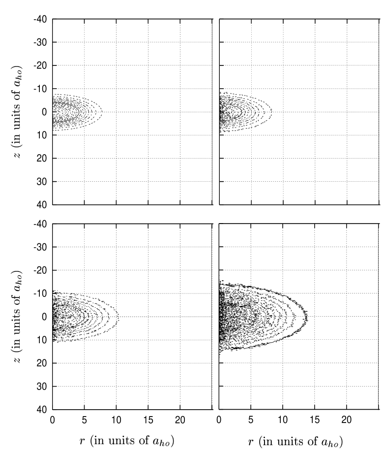
FIG. 3.: Expansion of a cold fermionic cloud after release from a harmonic trap: snapshots of the density distribution, shown as contour plots. From top left to bottom right: $t=0$, $5$, $10$ and $15$ ms. The axial and radial coordinates are in units of $a_{ho}$.

FIG. 4.: Expansion of a cold fermionic cloud and an inner condensate core after release from a harmonic trap: radial and axial widths of the density distributions (in units of $a_{ho}$) as functions of time. Circles: $\sigma_{r_{\perp}}$; squares: $\sigma_{z}$; open symbols: fermionic cloud; filled symbols: condensate; solid lines: analytical expressions (33) and (34) from Ref.[31].

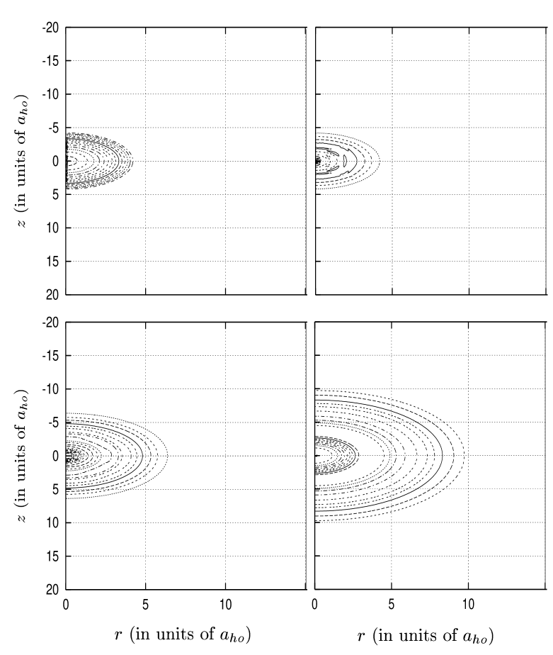
FIG. 5.: Expansion of a cold fermionic cloud with an inner condensate core after release from a harmonic trap: snapshots of the condensate density distribution, shown as contour plots. From top left to bottom right: $t=0$, $8.5$, $17$ and $25.5$ ms. The axial and radial coordinates are in units of $a_{ho}$.

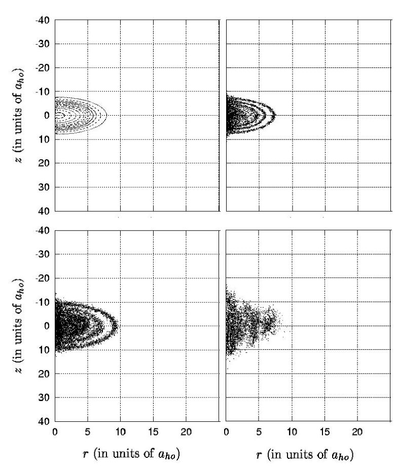
FIG. 6.: Expansion of a cold fermionic cloud with an inner condensate core after release from a harmonic trap: snapshots of the fermionic density distribution, shown as contour plots. From top left to bottom right: $t=0$, $8.5$, $17$ and $25.5$ ms. The axial and radial coordinates are in units of $a_{ho}$.

FIG. 7.: Oscillations of a condensate in a harmonic plus shallow optical-lattice potential: snapshots of the density distribution, shown as contour plots From top left to bottom right: $t=23.3$, $46.6$, $69.9$ and $93.2$ ms. The axial and radial coordinates are in units of $a_{ho}$.

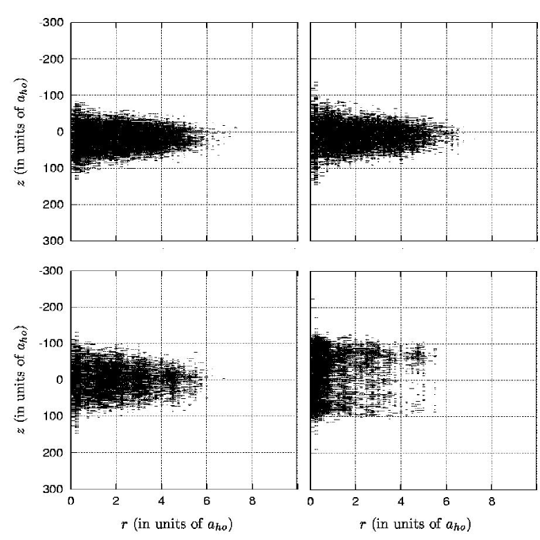
FIG. 8.: Oscillations of a bosonic thermal cloud in a harmonic plus shallow optical-lattice potential: snapshots of the density distributions, shown as contour plots. From top left to bottom right: $t=6$, $12$, $18$ and $24$ ms. The axial and radial coordinates are in units of $a_{ho}$.

FIG. 9.: Oscillations of a condensate in a harmonic plus deep optical-lattice potential: snapshots of the density distributions, shown as contour plots. From top left to bottom right: $t=23.3$, $46.6$, $69.9$ and $93.2$ ms. The axial and radial coordinates are in units of $a_{ho}$.

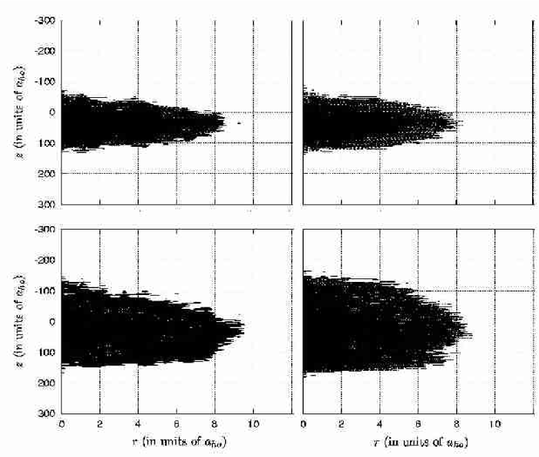
FIG. 10.: Oscillations of a bosonic thermal cloud in a harmonic plus deep optical-lattice potential: snapshots of the density distributions, shown as contour plots. From top left to bottom right: $t=2.8$, $5.6$, $8.4$ and $11.2$ ms. The axial and radial coordinates are in units of $a_{ho}$.

FIG. 11.: Oscillations of a condensate and a bosonic thermal cloud in a harmonic trap plus optical-lattice potential with: axial center-of-mass coordinate and average axial width of the density distributions (in units of $a_{ho}$) as functions of time. Continuous line, condensate with $\alpha=1$; dashed line, condensate with $\alpha=5$; crosses for the thermal cloud with $\alpha=1$ and circles for the thermal cloud with $\alpha=5$.

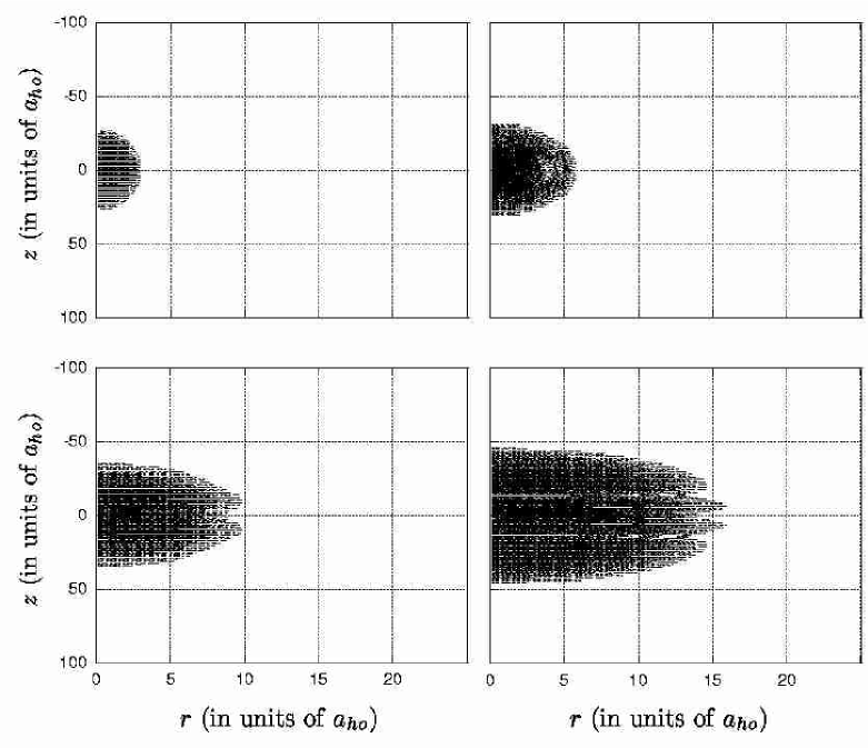
FIG. 12.: Expansion of a condensate interacting with its thermal cloud after release from harmonic plus deep optical-lattice potential: snapshots of the density distribution, shown as contour plots. From top left to bottom right: $t=0$, $3.5$, $7$ and $11.5$ ms. The axial and radial coordinates are in units of $a_{ho}$.

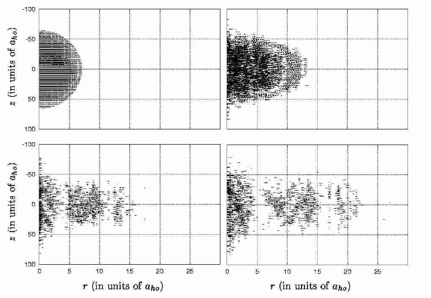
FIG. 13.: Expansion of a the bosonic thermal cloud interacting with a condensate after release from harmonic plus deep optical-lattice potentail: snapshots of the density distribution, shown as contour plots. From top left to bottom right: $t=0$, $3.5$, $7$ and $11.5$ ms. The axial and radial coordinates are in units of $a_{ho}$.

P	$N_{r}\times N_{z}$	CPU-time (hh:mm:ss)
$1.6\cdot 10^{6}$	201$\times$401	8:35:27
$8\cdot 10^{5}$	201$\times$401	5:33:55
$1.6\cdot 10^{6}$	401$\times$801	10:22:24

TABLE I.: Expansion of a cloud of fermionic ${}^{40}K$ atoms after release from the harmonic trap. CPU-time (third column) elapsed on a 1GHz Pentium III SCSI for simulating $20000$ time-steps, corresponding to $20\;ms$, for various numbers of computational particles (first column) and mesh sizes (second column).