[

Optimal combinations of imperfect objects

Abstract

We consider how to make best use of imperfect objects, such as defective analog and digital components. We show that perfect, or near-perfect, devices can be constructed by taking combinations of such defects. Any remaining objects can be recycled efficiently. In addition to its practical applications, our ‘defect combination problem’ provides a novel generalization of classical optimization problems. PACS numbers: 71.35.Lk, 71.35.Ee

]

Imperfection is an integral part of Nature, but it cannot always be tolerated. High-technology devices, for example, must be precise and dependable. The design of such dependable devices is the domain of fault-tolerant computing, where the goal is to optimize reliability, availability or efficiency of redundant systems [1]. Such redundant systems are typically built from devices which are initially defect-free and hence pass the quality check, but may later develop faults.

A much less studied problem, but one of significant economic and ecologic importance, is what to do with a component which is already known to be defective. Components with minor defects are sometimes acceptable for low-end devices [2]. The Teramac, a massively parallel computer, was built from partially defective conventional components; it uses an adaptive wiring scheme between the components in order to avoid the defects, and the wires themselves can be defective [3]. More typically, however, a component that is known to be defective is considered ‘useless’ and is hence wasted.

Here we address this wastage issue by relating it to a novel optimization problem: given a set of $N$ imperfect components, find a combination, or subset, that optimizes the average error (analog components), or the number of working transformations (digital components). We employ methods from statistical physics to show that perfect, or near-perfect, devices can indeed be constructed, and remaining objects can be recycled efficiently with (almost) zero net wastage. Note however that combining simple analog devices such as thermometers, is not attractive since it is usually much easier and cheaper to subtract the errors from the outputs. But such active error-correction may not be practical in more complex systems, particularly for next-generation technologies in the ultrasmall nano/micro regime. Nanoscale devices such as Coulomb-blockade transistors may enable us to push back the limits of Moore’s law (see Ref. [4] for a review). However, the accuracy of the current produced at a given analog voltage will depend sensitively on the reliability of the nanostructure’s fabrication. Similarly, the discrete optical transitions in semiconductor quantum dots [5] can provide useful digital components for nanoscale classical computing [6]. However, digital switching can only occur if the energy levels coincide with the external light frequency. The accuracy of these energy levels also depends on the precision of fabrication. However even in self-assembled quantum dot structures, such as the ground-breaking virus-controlled self-assembly scheme of Ref. [7] where quantum dots are mass-produced, no two individual dots will ever be identical - each will contain an inherent, time-independent systematic defect as compared to the intended design. Yet it would be highly undesirable to discard such nanostructures given the potential applications of such ‘bio-nano’ structures.

Consider an analog device such as a nanoscale transistor, registering a current $A+a$ given a particular applied voltage, with $A$ being the actual value and $a$ being the systematic error[8]. Suppose fabrication has produced a batch of $N$ imprecise devices whose errors $a_{i}$ ($i=1,2,\cdots N$) were created when the objects were built and remain constant; this amounts to drawing them from a known distribution $P(a)$. For simplicity, we suppose that $P(a)$ is Gaussian with average $\mu$ and variance $\sigma=1$[9]. The most precise component has an error of order $\frac{1}{N}$. What should one do with the others? Generally speaking, one could combine them such that their defects compensate. Computing the average of all components leads to an error of order $\mu\pm\frac{1}{\sqrt{N}}$ which vanishes very slowly for large $N$, and even then only if $\mu=0$. Nevertheless this method has been used in many contexts throughout history, for example by sailors who often took several clocks on board ship [10].

The optimal combination is actually obtained by taking a well-chosen subset of the $N$ components, i.e. a subset containing $M\leq N$ devices whose errors compensate best. The problem therefore consists of selecting some of the numbers $a_{i}$ such that the absolute value of their average is minimized: hence the interesting quantity is

$$\epsilon=\min_{\{n_{i}\}}\frac{|\sum_{j=1}^{N}n_{j}a_{j}|}{\sum_{k=1}^{N}n_{k}}=\min_{\{n_{i}\}}\frac{E}{M}\ \ .$$ (1)

Here $n_{j}\in\{0,1\}$ selects whether device $j$ is used or not, while $M=\sum_{i=1}^{N}n_{i}$ is the total number of devices used. Without division by $M$, this problem — which we call the defect combination problem (DCP) — would be similar to the subset sum problem or number partitioning problem (NPP) [11]. Both problems are equivalent and known to be NP-complete: in the worst case, there is no method which finds the minimum in polynomial time, i.e. significantly faster than brute force enumeration (exponential time). However the typical, i.e. average, problem has a different behavior. It will undergo a transition between a computationally hard phase where the average error is greater than zero, and a computationally easy phase where the error is zero [12, 13]. The same applies in our present case. These two phases, and the transition between them, can be studied using statistical physics [12, 13, 14, 15].

FIG. 1.: Unconstrained problem: the average error $\langle{\epsilon}\rangle$ versus the total number of components $N$ obtained by numerical evaluation. Average taken over 20000 samples. The solid line shows the behavior of the theoretical upper bound, for a particular choice of the constant $C$.

Figure 1 reports numerical results obtained by enumerating all possible $\{n_{i}\}$, where $\mu=0$. The resulting device precision can be quite remarkable. Our numerical simulations also confirm that $\langle{M}\rangle=N/2$ for large $N$, i.e. the optimal configuration uses half the components on average. Strong fluctuations remain even for a large number of realizations and for large $N$, because of the non self-averaging nature of the problem: i.e. $\sqrt{\langle{\epsilon^{2}}\rangle-\langle{\epsilon}\rangle^{2}}/\langle{\epsilon}\rangle\to 1$.

The division by $M$ in Eq (1) makes the DCP much harder to tackle analytically than the NPP. Let us compare the DCP with ${\rm min}E$, the problem defined by finding the minimum of $E$. Numerical simulations show that for the latter problem $\langle{M^{*}}\rangle_{a,\text{minE}}=\frac{N-1}{2}$ for sufficiently large $N$, where $M^{*}=\sum_{j=1}^{N}n_{j}^{*}$ is the number of selected components in the configuration $\{n_{i}^{*}\}$ that minimizes $E$ [16]. This makes sense, since in the DCP the division by $M$ favors configurations with a larger number of components. In addition both problems are related by the inequality

$$\min_{\{n_{i}\}}\left[{\frac{E}{M}}\right]\leq\frac{\min_{\{n_{i}\}}E}{M^{*}}\ \ .$$ (2)

Hence

$$\langle{\epsilon}\rangle\leq\frac{C}{N}\,\langle{\min_{\{n_{i}\}}E}\rangle$$ (3)

for some constant $C$. Computing the typical properties of ${\rm min}E$ hence yields an upper bound to the average optimal error. Following Ref. [13], we computed the partition function $Z=\sum_{\{n_{i}\}}\text{e}^{-\beta|\sum_{j}n_{j}a_{j}|}$, which for large $N$ yields

$$Z\simeq 2^{N}\int_{\pi/2}^{\pi/2}\text{e}^{NG(y)}$$ (4)

where $G(y)=\langle{\ln(\cos(a\beta\tan(y)/2))}\rangle$. Using the saddle point approximation for $Z$ and an argument of positive entropy [13], we find $\langle{\min_{\{n_{i}\}}E}\rangle\simeq\sqrt{\frac{\pi N}{2}}\,2^{-N}$. Hence there is a constant $C$ such that

$$\langle{\epsilon}\rangle\leq C\,\frac{1}{\sqrt{N}\,2^{N}}.$$ (5)

Figure 1 shows the behavior of the analytically obtained upper-bound for the average error is consistent with the corresponding numerical results. The same calculus shows that the DCP will also exhibit a phase transition between hard and easy problems when $b<N-\ln(\pi N/6)/2$, where $b$ is the number of bits needed to encode the $a_{i}$’s. Hence it is possible to obtain perfect error-free combinations of such imperfect objects for $N$ large and $b$ sufficiently small. When the defects are biased, i.e. $\mu\neq 0$, the error increases as $\mu$ increases but remains low for $\mu\leq 1$. When the errors of the components all have the same sign, only one component is used and the resulting error increases linearly with $\mu$.

We now consider the constrained DCP, where the number of components to be used is pre-defined to be a particular value $M$. If $M=1$, one selects the least imprecise component. The case $M=N$ amounts to computing the average over all $N$ components, hence $\langle{\epsilon}\rangle=\sqrt{2/(\pi N)}$. This problem is a more complicated version of the subset sum problem: in our case the numbers $a_{i}$ are no longer restricted to be positive and the cost function is the absolute value of the sum. Fig. 2 plots the average and median optimal error as a function of $M$ for $N=10$ and 20. An exponential fit of the minimum error for increasing $N$ gives $\min_{M}\langle{\epsilon}\rangle\sim\exp(-KN)$ where $K=0.56\pm 0.01$, to be compared with $-\ln 2=0.693\ldots$ in the unconstrained case; the functional form of this quantity may however be more complicated than an exponential.

We have also applied Derrida’s random cost approach [19, 18, 14]. Given the $N$ errors $\{a_{i}\}$, there corresponds one $E$ to each of the $L={N\choose M}$ sets $\{n_{i}^{\prime}\}$ that obey the constraint $\sum_{i}n_{i}^{\prime}=M$ [19, 18, 14]. If the $E$ are independent, all properties of the problem are then given by the p.d.f. $p_{M}(E)$. In our case, the latter is straightforward to compute:

$$p_{M}(E)={N\choose M}^{-1}\sum_{\{n_{i}^{\prime}\}}\langle{\delta(E-|\sum_{j}n_{j}a_{j}|)}\rangle,$$ (6)

where the prime means that $\sum_{i}n_{i}^{\prime}=M$. Hence $p_{M}(E)$ is equal to the probability distribution of the absolute value of $N$ numbers drawn from $P(a)$, which is

$$p_{M}(E)=\frac{\Theta(E)}{\sqrt{2\pi M}}\,\left[{\text{e}^{-\frac{(E-\mu M)^{2}}{2M}}+\text{e}^{-\frac{(E+\mu M)^{2}}{2M}}}\right]\ \ .$$ (7)

Let us concentrate on the non-biased case $\mu=0$ (the calculus is easily extended to the biased case). We are interested in the average value of the minimum $E_{1}$ of ${N\choose M}$ numbers drawn from $P_{M}(E)$. Using $P(E_{1})=-\frac{{\rm d}}{{\rm d}E_{1}}[F_{>}(E_{1})]^{L}$, where $F_{>}(E_{1})=\text{erfc}(E_{1}/\sqrt{2M})$ is the cumulative distribution function of $P_{M}(E)$, we find that

$$\frac{\langle{E_{1}}\rangle}{M}=\sqrt{\frac{2}{M}}\,\int_{0}^{\infty}{\rm d}t[\text{erfc}(t)]^{N\choose M}\ \ .$$ (8)

If $M=N$, one recovers the average over all components since $\int_{0}^{\infty}{\rm d}t\,\text{erfc}(t)=1/\sqrt{\pi}$. By definition, the median is given by $\epsilon_{\text{med}}$ such that $\int_{0}^{\epsilon_{\text{med}}}{\rm d}E_{1}\,P(E_{1})=1/2$.

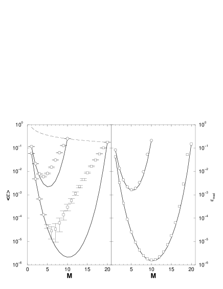
FIG. 2.: Constrained problem. Left panel: average optimal error $\langle{\epsilon}\rangle$ versus the number of components $M$ for a total of $N=10$ (circles) and 20 (squares) (average taken over 20000 samples). Right panel: median error versus $M$. Continuous lines are the predictions from the random cost approach. The dashed line is $\sqrt{\frac{2}{\pi N}}$, the average error is taken over all components.

The left panel of Fig. 2 plots the average constrained error, obtained by numerical enumeration, and the analytical predictions of Eq (8), for two sizes of component set. The larger the component pool $N$, the better the precision. For $M<<N$ the random cost approach describes $\langle{\epsilon}\rangle$ well, however it fails dramatically for larger values of $M$. This is because the $L={N\choose M}$ values of $E$ become increasingly dependent as $M/N$ grows. At fixed $N$, as $M$ increases, particular samples have an increasing probability to contain a large fraction of defects $a_{i}$ with the same sign. Due to the constraint on $M$, one may therefore be forced to use components whose defects add instead of compensating each other. The median, which is less affected by such events, has its mimimum close to $N/2$ (right panel of Fig. 2): the random cost approach describes much better the behavior of the median than that of the average, although the discrepancy increases as $M/N$ increases.

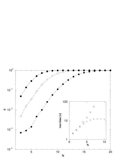
FIG. 3.: Binary components: average fraction $\langle{\phi}\rangle$ of perfect devices as a function of $N$ for $P=100$ and $f=0.2$ (filled circles), $f=0.25$ (squares) and $f=0.3$ (filled diamonds). Inset: running time versus $N$ of simple enumeration (x) and enumeration with sorting ($+$) ($f=0.2$). Averages taken over $10000$ samples. Dashed lines are for guidance to the eye.

Using a subset of defective components is also a powerful method for binary components such as quantum-dot optical switches [4, 6]. Suppose each component has $I$ input bits. If it can perform $F$ different logical operations on the input bits, it can perform $P=F2^{I}$ different transformations (i.e. truth table has $P$ entries). Let $f$ be the probability that for a given transformation $l$, component $i$ systematically gives the wrong output. e.g. because of inaccuracies in the energy-level spacings in the case of quantum dot switches. Mathematically, $P(a_{i}^{l}=-1)=f$, $-1$ labelling a defective ouput and $1$ a correct one. It becomes exponentially unlikely that one can extract a perfect component as $f$ increases, however subsets of the components may indeed produce the correct output. One therefore selects a subset of components from a pool of $N$, in order to maximize the number of transformation such that the majority of components give the correct answer. The maximal fraction of working transformations for a given set of components $\{a_{i}\}$ is

$$W(\{a_{i}\})=\frac{1}{P}\,\max_{\{n_{i}\}}\,\sum_{l=1}^{P}\Theta(\sum_{j=1}^{N}a_{j}^{l}n_{j})$$ (9)

where $\Theta(x)$ is the Heaviside function. We measured $\phi=\langle{\delta_{W,1}}\rangle$, the average fraction of component sets with at least one perfect subset. Numerical calculations confirm that it is indeed possible to build perfectly working components even if $f$ is so high that no single component is perfect. Figure 3 shows numerical simulations of the probability $\phi$ versus $N$ for three values of $f$. When $\phi>0$, an efficient algorithm consists in first ranking (Heapsort) the components according to the number of working transformations and then enumerate all possibilities until a perfect combination is found, beginning with the less defective ones (see inset of Fig 3). Analytic results along the lines of [19] will presented elsewhere.

Admittedly, seeking optimal combinations implies an additional cost for two reasons. First, one has to find the optimal or near optimal combination; this can be done either by measuring all the defects and then finding the minimal error with a computer; or, skipping the labour-intensive step of measuring individual defects, by building combinations of objects such that we eventually minimize the aggregate error. Second, these objects have to be wired, and their output combined by an additional hopefully error-free device. However such wiring and selection of working subsets of components, is precisely what is already being done inside the Teramac [3]. Given that defective components can be cheaply produced en masse, the cost of such wiring and selection of working combinations may not be an obstacle. Hence we believe that our two optimization problems may prove relevant in practice, in particular in emerging technologies where the fabrication of defect-free components may not be possible.

Our scheme implies that the ‘quality’ of a component is not determined solely by its own intrinsic error. Instead error becomes a collective property, which is determined by the ‘environment’ corresponding to the other defective components. Efficient recycling of otherwise ‘useless’ components now becomes possible. Suppose that a fabrication process produces a constant flow of defective analog or binary components. One can now perform the following scheme to generate a continuous output of useful devices: fix $N$ according to the desired average error (see Fig. 1, Fig. 2 or Fig 3); form the optimal subset; add fresh components to the unused ones; find the optimal subset, and repeat as desired. The quality of the subset fluctuates, but there is essentially no wastage. Although efficient algorithms for the analog case remain to be found, generalization of well-known algorithms [20] may be possible. We hope that our work inspires further academic research into this important practical problem.

We thank R. Zecchina and D. Sherrington for useful comments. D.C. thanks the Swiss National Funds for Scientific Research for financial support.

REFERENCES

- [1] B.W. Johnson, Design and Analysis of Fault Tolerant Digital Systems, Addison-Wesley, New York, 1989; P.Ch. Kandellakis and A.A. Shvartsman, Fault-Tolerant parallel computation, Kluwer, Boston, 1997; D.P. Siewiorek, and R.S. Swarz, Reliable Computer Systems, Digital Press, Burlington, 1992.
- [2] M. Breuer, Proceedings of the IEEE 18th VLSI Test Symposium VST00, IEEE Data Center, 2000.
- [3] J.R. Heath, P.J. Kuekes, G.S. Snider and R.S. Williams, Science 280, 1716 (1998).
- [4] Solid State Century, Sci. Am. Special Issue, October 1997.
- [5] N.F. Johnson, J. Phys.: Condens. Matt. 7, 965 (1995).
- [6] S.C. Benjamin and N.F. Johnson, Appl. Phys. Lett. 70, 2321 (1997); Phys. Rev. A 60, 4334 (1999).
- [7] S. Lee, C. Mao, C. Flynn and A. Belcher, Science 296, 892 (2002).
- [8] Our approach is easily extended to multifunction devices.
- [9] All results can be extended to the general case simply by multiplying and by .
- [10] J.-J. Liengme, private communication.
- [11] M.R. Garey and D.S. Johnson, Computers and Intractability. A Guide to the Theory of NP-Completeness, W. H. Freeman, New York (1997).
- [12] N. Karmakar, R. M. Karp, G. S. Lueker, A. M. Odlyzko, J. Appl. Prob. 23, 626 (1986).
- [13] S. Mertens, Phys. Rev. Lett. 81, 4281 (1998).
- [14] S. Mertens, Phys. Rev. Lett. 84, 1347 (2000).
- [15] R. Monasson, R. Zecchina, S. Kirkpatrick, B. Selman and L. Toyanski, Nature 400, 133 (1999).
- [16] The configuration minimizes .
- [17] B. Derrida, Phys. Rev. E 24, 2613 (1981).
- [18] D. Gross, M. Mézard, Nucl. Phys. B 240, 431 (1984).
- [19] E. Gardner, B. Derrida, J. Phys. A 21, 271 (1988)
- [20] N. Karmarkar, R. Karp, Technical Report UCB/CSD 81/113, Computer Science Division, U. California, Berkeley (1982); R. E. Korf, Artif. Intell. 106, 181 (1998); S. Mertens, e-print cs.Ds/9903011 (unpublished).