Preprint MPI-PhT/2002-06
Lessons of Coherence and Decoherence–From Neutrinos to SQUIDS

Abstract

We indicate some of the lessons learned from our work on coherence and decoherence in various fields and mention some recent work with solid state devices as elements of the “quantum computer”, including the realization of simple logic gates controlled by adiabatic processes. We correct a commonly held misconception concerning decoherence for a free particle.

Presented at the XXII Solvay Conference, The Physics of Information

Delphi, Nov 2001

The subject of “quantum information” and in particular its realization in terms of real devices revolves in large measure around the problems of coherence and decoherence . Thus it may be of interest here to review the origins of the subject and see what has been learned in applications to various areas. We first got involved in these issues through the attempt to see the effects of parity violation (“weak neutral currents”) in handed molecules [1]. The method we found–an analogy to the famous neutral $K$ meson behavior with chiral molecules– seemed too good to be true: we had a way of turning $10^{-15}$ Ev into a big effect! There must be some difficulty, we felt. Indeed there was; it turned out to be what we called “quantum damping” and what now-a-days is called “decoherence”.

The lessons from this work were several and interesting. First, concerning parity violation, we realized that this could solve Hund’s “paradox of the optical isomers” as to why we observe handed molecules when the true ground state should be parity even- or- odd linear combinations. We realized that for molecules where tunneling between chiral isomers is small, parity violation dominates and the stationary state of the molecule becomes a handed or chiral state, and not a 50-50 linear combination of chiral states.

This holds for a perfectly isolated molecule, and in itself has nothing to do with decoherence . However, and this is very related, even a very small interaction with the surroundings suffices to destroy the coherence necessary for the aforesaid linear combination, in effect the environment can stabilize the chiral states. This now goes under the catch-word “decoherence by the environment”. The limit of strong damping or stabilization is often called the Zeno or “watched pot” effect, an idea which as far as I can tell, goes back to Turing. We were able to show how this just arises as the strong damping limit of some simple “Bloch-like” equations [2, 3].

I The Unitarity Deficit Formula

A result of this work is that there is a simple and illuminating formula for the decoherence rate. There is a quantity $\Lambda$, given by the flux of the surrounding particles or excitations, and the $S$ matrix for the interaction of our system (e.g. the chiral molecule) with these surroundings:

$$\Lambda=i(flux)<i|(1-S_{L}S_{R}^{\dagger})|i>$$ (1)

The imaginary part gives the decoherence rate or loss of phase coherence per unit time $D$:

$$D=Im~{}\Lambda$$ (2)

(The real part also has a significance, a level shift induced by the surroundings. This turns out to be a neat way to find the index of refraction formula for a particle in a medium [6, 7].)

The labels (L,R) on the $S$ refer to which state of the molecule (or other system) is doing the interacting with the surroundings. Here with (L,R) we have taken the case of the simplest non-trivial system, the two-level system.

These equations may be derived[3, 6] by thinking of the S-matrix as the operator which transforms the initial state of an incoming object into the final state. If the different states (L,R) of our system scatter the object differently, a “lack of overlap” or “unitarity deficit” as given by Eq [1] arises. These intuitive arguments can also supported by more formal manipulations [7].

An important point that we see here, in Eq [1], is that the environment “chooses a direction in hilbert space”[6]. That is, there is some direction (here L,R) in the internal space of the system under study (the molecule) that is left unchanged–is not “flipped”– by the interaction with the surroundings. Such states however get a phase factor by the interaction, and this is the decoherence . If the interaction did not distinguish some direction, if we had $S_{L}=S_{R}$ then the formula tells us there would be no decoherence . This is intuitively correct in accord with one’s ideas about “measurement”. If the probe does not distinguish any state there are no “wavefunction collapses” and no decoherence takes place. (This is not meant to imply sanctioning of “wavefunction collapses” in any way.)

Another simple limit for the formula occurs when only one state interacts, say no interaction for L, or $S_{L}=1$. Then one finds that the decoherence rate is 1/2 the scattering rate for the interacting component [3]. Thus Eqs [1,2] have two interesting limits:

$$S_{L}=S_{R}~{}~{}~{}~{}~{}~{}~{}~{}~{}~{}~{}~{}~{}~{}~{}~{}~{}D=0\;,~{}~{}no~{}decoherence$$ (3)

and

$$S_{L}=1~{}~{}~{}~{}~{}~{}~{}~{}~{}~{}~{}~{}~{}~{}D=1/2~{}(scattering~{}rate~{}of~{}R)$$ (4)

The latter followed from an application of the optical theorem. With appropriate evaluation of the S-matrices, Eqs [1,2] can be applied to many types of problems, like quantum dots [11] or neutrinos [4], or even gravity [8].

Eq [3] is quite interesting in that it says the system can interact but nevertheless retain its internal coherence. A lesson here is that one shouldn’t think that every interaction or disturbance “decoheres” or “reduces” the system. The system can interact quite a bit as long as the interactions don’t distinguish the different internal states.

II A common misconception

The fact that the interaction responsible for the decoherence must “choose a direction in hilbert space” has some interesting implications. One of these has to do with the decoherence of a free particle in some background environment.

Eq [1] was for a two-state system, and the extension to a larger number of states, as long as it is a finite number, can be easily envisioned as following the logic[2, 3, 6] used in finding Eq [1]. However if we go to the continuum, that is if we have a infinite number of states, the problem becomes more subtle. The most common example of this is the free particle which, say in the limit of an infinitely large “box”, is described as system of continuous, dense, levels.

A number of authors, in talking about this system, have automatically assumed, as indeed first seems plausible, that at long times the particle under the influence of some continually interacting environment becomes totally “decohered”; in the sense that the density matrix of the particle $\rho(x,x^{\prime})$ approaches the situation of no off-diagonal elements, that $\rho$ approaches a $\delta$ function.

Although this may seem plausible, that under the repeated bombardment by the surroundings the particle becomes more and more “decohered”, it is in fact wrong

$$\rho(x,x^{\prime})\rightarrow\sim\delta(x-x^{\prime})~{}~{}~{}~{}~{}~{}~{}~{}~{}~{}~{}~{}~{}~{}~{}~{}~{}~{}~{}wrong$$ (5)

Consider the simplest case, that of a thermal environment. On general grounds we expect the particle in a thermal environment to be described by the boltzmann factor, to be given by a density matrix operator $\rho\sim e^{-H/T}$, where T is the temperature and H the hamiltonian, say $p^{2}/2m$ for a non-relativistic particle. Now evaluate this operator in the position representation:

$$\rho(x,x^{\prime})=<x|e^{-p^{2}/2mT}|x^{\prime}>\sim\int d^{3}p~{}e^{i{\bf p(x-x^{\prime})}-p^{2}/2mT}\sim e^{-(x-x^{\prime})^{2}MT/2}$$ (6)

This is the stationary, long time value of $\rho$. It applies for nearly any state we care to initially throw into the medium. Evidently it shows no signs of changing and certainly no sign of turning into a $\delta$ function. Of course at high temperature our expression will resemble a delta function. The practical importance of this will depend on the other length scales in the problem at hand. The point we wish to make, however, is of a conceptual nature, namely that repeated interactions with the environment don’t necessarily lead to more “decoherence”. Indeed Eq [6] says if we were initially to put $\delta(x-x^{\prime})$ or some other “highly incoherent” density matrix into the medium, the density matrix of the particle would become more coherent with time— until it reached the value Eq [6]. Apparently the medium can “give coherence” to a state that never had any to start with.

“Creating coherence” by an outside influence is not as mysterious as it may sound, there are familiar cases where we know this already. For example, using a high resolution detector can “create a long wavepacket” [5] or in particle physics neutral $K$ oscillations and the like may be enhanced or “created” by using some subset of our total event sample, such as a “flavor tag”.

Where did the seemingly plausible argument or feeling about the indefinitely increasing decoherence go wrong? It’s the question of the “direction chosen in hilbert space”. The feeling is right, but we must know where to apply it. As we can see from the boltzmann factor, thermodynamics likes to work in momentum (actually energy) space. The intuition would have been right there,–in momentum space– but this then means something non-trivial in position space. The lesson here is that the notion of “decoherence by the environment” must be understood to include a statement about the “direction chosen in hilbert space” by that environment [6].

III Mesoscopic systems

The interest in these issues has had a revival with the advances made possible by the technologies of mesoscopic systems. In one such system, the “quantum dot observed by the QPC”, one has a complete model of the measurement process, including the “observer”, “who” in this case is a quantum point contact (QPC) [10]. In a slight generalization of the original experiment  [9] one can see how not only the density matrix of the object being observed is “reduced” by the observing process, but also see how the readout current–the “observer” responds. In particular one may see how effects looking very much like the “collapse of the wavefunction”, that is sequences of repeated or “telegraphic” signals indicating one or another of the two states of the quantum dot, arise. All this without putting in any “collapses” by hand [11].

We should stress that what we are not only talking about a reduction of fringe contrast due to “observing” or disturbing an interference experiment, as in  [9]; and also in interesting experiments in quantum optics where an environment is simulated [12] or different branches of the interferometer  [13] interact differently and adjustably with the radiation in a cavity (like our two S-matrices). By the “collapses” however, we are referring not so much to the interferometer itself as to the signal from some “observing” system, like the current in the qpc. With repeated probing of the same object (say electron or atom), in the limit of strong “observation” this signal repeats itself —-this is the “collapse”. For not too strong observation there is an intermediate character of the signal, and so on. All this may be understood by considering the amplitude for the interference arrangement and the readout procedure to give a certain result  [11]. The properties of the readout signal naturally stand in some relation to the loss of coherence or “fringe contrast” of the interference effect under study.

Following this line of thought we come to the idea that there should be some relation between the fluctuations of a readout signal and decoherence. Indeed the decoherence rate, the imaginary part of Eq [1] is a dissipative parameter in some sense; it characterizes the rate of loss of coherence. Now there is the famous “dissipation- fluctuation theorem”, which says that dissipative parameters are related to fluctuations in the system. Is there some such relationship here? Indeed, one is able to derive a relation between the fluctuations of the readout current and the value of $D$[14]. The interesting and perhaps practical lesson here is that the decoherence parameter can be observed in two ways. One is the direct way, just observe the damping out of the coherent oscillations of the system in question. Experimentally, this involves starting the system in a definite, selected state. However, as just explained, there is a second way; namely observe the fluctuations of the readout. This can be done even if the system is in the totally “decohered” $\rho\sim I$ state.

Another mesoscopic system, the SQUID and in particular the rf SQUID, has been long discussed[15] as a candidate for showing that even macroscopic objects are subject to the rules of quantum mechanics. The rf SQUID, a Josephson device where a supercurrent goes around a ring, can have two distinct states, right- or left- circulation of the current. These two conditions apparently differ greatly, since a macroscopic number of electrons change direction. It would be a powerful argument for the universality of the quantum rules if one could demonstrate the meaningfulness of quantum linear combinations of these two states.

Such linear combinations can in principle be produced since there is some amplitude for a tunneling between the two configurations. In fact this was recently manifested through the observation of the “repulsion of levels” to be anticipated if the configurations of opposite current do behave as quantum states[16].

Another approach, where we would directly “see” the meaningfulness of the relative quantum phase of the two configurations, is the method of “adiabatic inversion” [17, 18]. This method also offers the possibility of a direct measurement of the decoherence time. In adiabatic inversion the “spin” representing a two-level system [3], [4] is made to “follow” a slowly moving “magnetic field” (meant symbolically, as an analogy to spin precession physics), which is swept from “up” to “down”. In this way the system can be made to invert its direction in “spin space”, that is to reverse states and go from one direction of circulation of the current to the other. This inversion is an intrinsically quantum phenomenon. If it occurs it shows that the phases between the two configurations were physically meaningful and that they behave quantum mechanically . This may be dramatically manifested if we let decoherence destroy the phase relation between the two configurations. Now the configurations act classically and the inversion is blocked.

We thus predict that when the decoherence rate is low the inversion takes place, and when it is high it does not. Figs 1 and 2 show the idea of this procedure.

FIG. 1.: A successful inversion, starting from the upper figure and ending with the lower figure. The black dot indicates which state is occupied. The system starts in the lowest energy level and by staying there, reverses states. It behaves as a quantum system with definite phase relations between the two configurations.

FIG. 2.: An inhibited inversion, starting from the upper figure and ending with the lower figure. Due to the lack of phase coherence the system behaves classically and stays in the same state, the current is not reversed.

Since in such an experiment we have the sweep speed at our disposal, we have a way of determining the decoherence time. It is simply the slowest sweep time for which the inversion is successful. We must only be sure that for the sweep speeds in question the the conditions remain adiabatic.

Setting up the adiabatic condition and taking some estimates for the decoherence time, it appears that the various requirements can be met  [17], [18] when operating at low temperature. Hence it may be realistically possible to move between the classical and quantum mechanical worlds–to turn quantum mechanics “on and off” in one experiment. This would be a beautiful experiment, the main open question being if the estimates of the decoherence rate are in fact realistic, since we are entering a realm which has not been explored before.

IV Adiabatic logic elements and the quantum computer

A two-state system behaving quantum mechanically can serve as the physical embodiment of a quantum mechanical bit, the “qbit”. Furthermore, the adiabatic inversion procedure just described amounts to a quantum realization of one of the basic elements of computer logic: the NOT. If one configuration is identified as 1 and the other as 0, then the inversion turns a linear combination of 1 and 0 into a linear combination of 0 and 1 with reversed weights.

We can try to push this idea of “adiabatic logic” a step further. NOT was a one bit operation. The next most complicated logic operation is a two bit operation, which we may take to be “controlled not” or CNOT. In CNOT the two bits are called the control bit and the target bit, and the operation consists of performing or not performing a NOT on the target bit, according to the state of the control bit.

To realize CNOT, an idea which suggests itself [17] as a generalization of adiabatic inversion is the following. We have a two bit operation and so two SQUIDS. These are devices with magnetic fields. Now if one SQUID, the target bit, is undergoing a NOT operation, it can be influenced by the control bit, a second nearby SQUID, through its linking flux. We could imagine that this linking flux can be arranged so that it helps or hinders the NOT operation according to the state of the second SQUID. This would amount to a realization of “controlled not”, again by means of an adiabatic sweep.

To analyze this proposal we must set up the two-variable Schroedinger equation describing the two devices and their interaction. The result is a hamiltonian with the usual kinetic energy terms and a potential energy term in the two variables, which in this case are the fluxes in the SQUIDS, $\phi_{1},\phi_{2}$:

$$V={1\over 2}V_{0}\bigl{\{}[l_{1}(\phi_{1}-\phi^{ext}_{1})^{2}+l_{2}(\phi_{2}-\phi^{ext}_{2})^{2}-2l_{12}(\phi_{2}-\phi^{ext}_{2})(\phi_{1}-\phi^{ext}_{1})]+\beta_{1}f(\phi_{1})+\beta_{2}f(\phi_{2})\bigr{\}}\;.$$ (7)

The $\phi^{ext}$ are external biases which in general will be time varying. The $l^{\prime}s$ are dimensionless inductances and $l_{12}$ represents the coupling between the two devices. The $f(\phi)$ are symmetric functions starting at one and decreasing with increasing $\phi$ so as to produce a double well potential when combined with the quadratic term; in the SQUID $f(\phi)=cos(\phi)$. Fig. 3 shows this “potential landscape” for some typical values of the parameters.

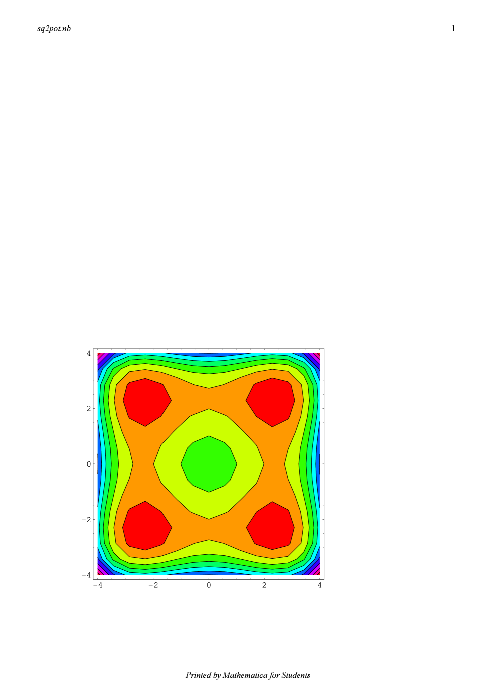
FIG. 3.: Potential landscape for CNOT

Given the hamiltonian, we must search for values of the control parameters $\phi^{ext}$, the “external fields”, which can be adiabatically varied in such a way as to produce CNOT. Preliminary analysis indicates favorable regimes of the rather complex parameter space where this can in fact be done [19].

V Some Experimental Proposals

Finally we would like to recall that there are still some fundamental and beautiful experiments waiting to be done in these areas.

A) One is the demonstration of the large effects of parity violation for appropriately chosen and contained handed molecules [1]. Because of what we now call decoherence this seemed very remote at the time. But now with the existence of single atom/molecule traps and related techniques, perhaps it’s not so hopeless.

B) Another, concerned with fundamentals of quantum mechanics, could be called the “adjustable collapse of the wavefunction” where the “strength of observing” can be varied, leading to effects like washing out of interferences, as already seen in [9] and a number of further predictions where we vary the qualities of the “observer” [11], or slowing down of relaxation according to the rate of probing of the object [3].

C) Then there is the second way of measuring $D$, through the fluctuations in the readout signal, even for a fully “decohered” system.

D) Finally there is the direct demonstration of quantum linear combinations of big objects by the method of adiabatic inversion; “turning quantum mechanics on and off” [17, 18].

Many of the questions we have briefly touched upon had their origins in an unease with certain consequences of quantum mechanics, often as “paradoxes” and “puzzles”. It is amusing to see how, as we get used to them, the “paradoxes” fade and yield to a more concrete understanding, sometimes even with consequences for practical physics or engineering. If we avoid overselling and some tendency to an inflation of vocabulary, we can anticipate a bright and interesting future for “applied fundamentals of quantum mechanics”.

REFERENCES

- [1] Quantum Beats in Optical Activity and Weak Interactions, R.A. Harris and L.Stodolsky, Phys Let B78 (1978) 313. [Molecular tunneling and parity violation, need to understand decoherence.]
- [2] On the Time Dependence of Optical Activity, R.A. Harris and L.Stodolsky, J. Chem. Phys. 74 (4), 2145 (1981).[Decoherence by environment, formula for decoherence rate, application to chiral molecules.] The notion that handed molecules could “decohere” or be stabilized by the environment somehow was raised by H.D.Zeh, Found. Phys. 1,69 (1970), M. Simonius, Phys Rev. Lett. 40, 980 (1978).
- [3] Two Level Systems in Media and ‘Turing’s Paradox’, R.A. Harris and L.Stodolsky, Phys. Let. B 116(1982)464.[Decoherence by environment, formula for decoherence rate, quantitative explanation of “Zeno”, prediction of anti-intuitive relaxation, application to neutrinos.]
- [4] On the Treatment of Neutrino Oscillations in a Thermal Environment, L.Stodolsky, Phys. Rev. D 36(1987)2273 .[Method for decoherence in neutrino oscillations. Spin precession picture for neutrinos.] See chapter 9 of G.G. Raffelt, Stars as Laboratories for Fundamental Physics (Univ. Chicago Press, 1996)
- [5] When the Wavepacket is Unnecessary, L.Stodolsky, Phys. Rev. D58 036006, 1998 and hep-ph/9802387.
- [6] Quantum Damping and Its Paradoxes, L.Stodolsky, in Quantum Coherence, J. S. Anandan ed. World Scientific, Singapore (1990)[Review and historical background to 1989.]
- [7] Non-Abelian Boltzmann Equation for Mixing and Decoherence G. Raffelt, G. Sigl and L.Stodolsky, Phys Rev Let. 70(1993)2363.[Derivation of decoherence rate formula in neutrino applications ]
- [8] Decoherence Rate of Mass Superpositions, L.Stodolsky, Acta Physica Polonica B27,1915(1996). [Decoherence in gravitational interactions.]
- [9] S. Gurvitz, quant-ph 9607029. E. Buks, R. Schuster, M. Heiblum, D. Mahalum and V. Umanksy, Nature 391, 871 (1998).
- [10] M. Field, C.G. Smith, M. Pepper, D. A. Ritchie, J. E. F. Frost G.A. C. Jones and D.G. Hasko, Phys. Rev. Lett. 70, 1311 (1993).
- [11] Measurement Process In a Variable-Barrier System, L.Stodolsky, Phys. Lett. B459 pages 193-200, (1999). [Formalism for quantum dot-QPC system. Prediction of novel phase effect. Prediction of “collapse-like” behavior of readout.]
- [12] Myatt et al. Nature 403, 269 (2000).
- [13] Brune et al. Phys. Rev. Lett. 77, 4887 (1996).
- [14] Decoherence-Fluctuation Relation and Measurement Noise, L.Stodolsky, Physics Reports 320 51-58 (1999), quant-ph/9903075. [Suggestion of Decoherence-Fluctuation Relation connecting decoherence rate and fluctuations of readout signal.]
- [15] See A. J. Leggett, Les Houches, session XLVI (1986) Le Hasard et La Matiere; North -Holland (1987), references cited therein, and introductory talk, Conference on Macroscopic Quantum Coherence and Computing, Naples, June 2000, Proceedings published by Academic-Plenum.)
- [16] J. Friedman, V. Patel, W.Chen, S.K. Tolpygo and J.E. Lukens, Nature 406, 43 (2000). C.S. van der Wal, A.C. ter Haar, F. K. Wilhelm, R. N. Schouten, C.J.P.M. Harmans, T.P. Orlando, Seth Lloyd, and J.E. Mooij, Science 290 773 (2000) and in MQC2: Conference on Macroscopic Quantum Coherence and Computing, Naples, June 2000, Proceedings published by Academic-Plenum.
- [17] Study of Macroscopic Coherence and Decoherence in the SQUID by Adiabatic Inversion, Paolo Silvestrini and L.Stodolsky, Physics Letters A280 17-22 (2001).[Linear Combinations of macroscopic states. Measuring decoherence time. Relation to NOT operation.] cond-mat/0004472
- [18] Adiabatic Inversion in the SQUID, Macroscopic Coherence and Decoherence, Paolo Silvestrini and L.Stodolsky, Macroscopic Quantum Coherence and Quantum Computing, pg.271, Eds. D. Averin, B. Ruggiero and P. Silvestrini, Kluwer Academic/Plenum, New York (2001). [Linear Combinations of macroscopic states. Measuring decoherence time.]cond-mat/0010129. D.V. Averin, Solid State Communications 105, 659 (1998), has discussed related ideas using adiabatic operations on the charge states of small Josephson junctions.
- [19] Adiabatic Methods for a Quantum CNOT Gate, Valentina Corato, Paolo Silvestrini, L.Stodolsky, and Jacek Wosiek, cond-mat/0205514, and contribution to Macroscopic Quantum Coherence and Quantum Computing 2002. [ Principles of quantum gates using adiabatic inversion. Design parameters for CNOT.]