Theory and simulation of the nematic anchoring coefficient

Abstract

Combining molecular simulation, Onsager theory and the elastic description of nematic liquid crystals, we study the dependence of the nematic liquid crystal elastic constants and the zenithal surface anchoring coefficient on the value of the bulk order parameter.

I Introduction

The anchoring phenomenon is the tendency of a liquid crystal to orient in a particular direction when in contact with the container walls. The equilibrium director orientation set by the interaction of the liquid crystal with the aligning surface is called an easy orientation axis. The simplest, strong anchoring, assumption is that the director has a fixed orientation at the boundaries along the easy orientation axis. However, it has been discovered that the coupling of the director with the orienting surface can be rather weak. This results in deviation of the surface director from the easy axis in response to small perturbations.

On a phenomenological level, weak anchoring can be described by adding an appropriate surface potential to the free energy of the system. Then minimization of the free energy functional gives both the equations for the director in the bulk and the appropriate boundary conditions de Gennes and Prost (1995). The simplest form of the surface potential has been proposed by Rapini and Papoular Rapini and Papoular (1969)

$$f_{\rm{s}}=-\frac{1}{2}W(\bm{n}\cdot\bm{e})^{2},$$ (1)

where the parameter, $W$, is termed an anchoring energy.

Since then, numerous experimental methods have been used to measure the surface anchoring coefficient $W$ Subacius et al. (1995); Yokoyama and van Sprang (1985); Nastishin et al. (1999); its value has turned out to be extremely important for liquid crystal devices, i.e. displays, optical switches. However, comparatively little work on systematic experimental investigation of the anchoring phenomenon has been presented up till now. From the available experimental data, one can say that the extrapolation length $\lambda=K_{33}/W$ is inversely proportional to the squared value of the bulk order parameter $\lambda\propto Q^{-2}$. Taking into account that the elastic constant $K_{33}$ is typically proportional to $Q^{2}$, this gives for the anchoring parameter $W\propto Q^{4}$ Mertelj and Čopič (2000).

There have been several attempts to estimate the anchoring coefficient theoretically Tjipto-Margo and Sullivan (1988) and by combining molecular simulation with a local density functional approach Stelzer et al. (1997); Teixeira et al. (2001). The main difficulty here is that one needs to know the direct pair correlation function of the nematic state, which is usually unknown, and must hence be estimated with some uncontrolled approximations or assumptions (see, however, Ref. Phuong et al. (2001)). Moreover, it is often assumed that the director in the interface region is fixed Stelzer et al. (1997). However, it has already been noticed that these approximations may give incorrect results, by at least an order of magnitude, for example in the calculation of bulk elastic constants Phuong et al. (2001).

Similar studies have also been done using lattice models. The existence of subsurface deformations and effective intrinsic anchoring arising from the incomplete molecular interaction close to the surface has been studied using a hexagonal lattice approach Skačej et al. (1997). Monte-Carlo simulations of the Lebwohl-Lasher model have shown that the extrapolation length is not in general equal to the ratio of the bulk to surface couplings Priezjev and Pelcovits (2000). However, the results were not sufficiently robust to determine the dependence of the anchoring energy on the order parameter.

The present work attempts to remedy the situation by combining the elastic description with Onsager theory and Monte Carlo simulation results. We study the dependence of the elastic ($K_{33}$) and surface anchoring ($W$) coefficients on the liquid crystal state point, which is defined by the bulk value of the order parameter $Q$.

The paper is organized as follows. We define the geometry and derive director profiles using elastic theory in section II. In section III we discuss the Onsager approach which allows us to calculate the single particle density of the bulk and confined systems, while section IV outlines the fluctuation approach to calculating elastic coefficients. Section V gives details of the technique used in Monte Carlo simulations and the results are summarized in section VI.

II Elastic description

The easiest way to obtain the surface anchoring coefficient $W$ is to create a director deformation far from the surface. Then, measuring the response of the director near the cell surface, or fitting the director profile with a theoretically predicted profile, yields an estimate of the anchoring extrapolation length and ratios of the elastic constants.

Indeed, consider one of the possible geometries suitable for the measurement of the zenithal anchoring strength. Let the director have fixed orientation at the boundary $z=L$. The surface at $z=0$ is assumed to provide homeotropic anchoring of strength $W$. In the elastic description, deformations of the director field $\bm{n}$ are described by the total free energy de Gennes and Prost (1995)

$${\cal F}_{\text{el}}=\int_{V}\,f_{\text{b}}\,dV+\int_{S}\,f_{\text{s}}\,dS\>.$$ (2)

Here $f_{\text{b}}$ is the Frank-Oseen elastic free energy density

$$f_{\text{b}} = \frac{1}{2}\left\{K_{11}\left(\nabla\cdot\bm{n}\right)^{2}+K_{22}\left(\bm{n}\cdot\left[\nabla\times\bm{n}\right]\right)^{2}+\right.$$

$$\left.+K_{33}\left[\bm{n}\times\left[\nabla\times\bm{n}\right]\right]^{2}\right\},$$

where $K_{11}$, $K_{22}$, and $K_{33}$ are elastic constants, and the integration extends over the sample volume $V$. $f_{\text{s}}$ is the surface anchoring energy density, which we assume to be of the Rapini-Papoular form (1), and it is integrated over the boundary surface $S$.

In slab geometry, the director $\bm{n}$ is assumed to lie in the $xz$ plane and depends only on the $z$ coordinate. Then it can be parametrized as $\bm{n}=(\sin\theta,0,\cos\theta)$ which transforms eqn (2) into a free energy per unit area

$${\cal F}_{\text{el}}/S=\frac{1}{2}K_{33}\int_{0}^{L}{f_{13}(\theta)\left(\frac{\partial\theta}{\partial z}\right)}^{2}{dz}-\frac{1}{2}W\cos^{2}\theta_{0},$$ (4)

where $f_{13}(\theta)=1-\delta\sin^{2}\theta$, $\delta=(K_{33}-K_{11})/K_{33}$, $\theta_{0}=\theta(z=0)$.

The absence of explicit $z$-dependence in the free energy (4) implies the first integral

$${f_{13}(\theta)\left(\frac{\partial\theta}{\partial z}\right)}^{2}=\text{const}.$$ (5)

Boundary conditions read

$$K_{33}{f_{13}(\theta_{0})\left.\frac{\partial\theta}{\partial z}\right|_{z=0}} = \frac{1}{2}W\sin 2\theta_{0},$$ (6)

$$\theta(z=L) = \theta_{L}.$$

Here we assumed that the director angle at the boundary $z=L$ is fixed.

Integrating eqn (5), together with the boundary conditions, yields

$$E(\theta,\delta)=E(\theta_{0},\delta)+[E(\theta_{L},\delta)-E(\theta_{0},\delta)]z/L,$$ (7)

$${[E(\theta_{L},\delta)-E(\theta_{0},\delta)]}\sqrt{f_{13}(\theta_{0})}=(L/2\lambda)\sin 2\theta_{0},$$

where $E(\theta,\delta)=\int_{0}^{\theta}\sqrt{f_{13}(x)}dx$ is the incomplete elliptic integral of the second kind, and $\lambda=K_{33}/W$ is the anchoring extrapolation length. For small angles $\theta_{0}$ eqn (7) can be simplified and has the form

$$E(\theta,\delta)=E(\theta_{L},\delta)\frac{z+\lambda}{L+\lambda}.$$ (8)

Note, that for small angles $\theta_{L}$ and, correspondingly, for small $\theta$, $E(\theta,\delta)=\theta$ and we have linear dependence of the director angle on the $z$ coordinate

$$\delta n_{x}(z)\approx\theta(z)=\theta_{L}\frac{z+\lambda}{L+\lambda}.$$ (9)

Using eqn (8), one can fit the director profiles $\theta(z)$ with $\lambda=K_{33}/W$ and $\delta=(K_{33}-K_{11})/K_{33}$ as adjustable parameters. To simplify the procedure, it is more appropriate to fit $z(\theta)$ rather than $\theta(z)$.

III Onsager approach

The Helmholtz free energy in the Onsager approach is expressed in terms of the single-particle density, $\rho(\bm{1})$, where $(\bm{1})=(\bm{r}_{1},\bm{\Omega}_{1})$ represents both position $\bm{r}_{1}$ and orientation $\bm{\Omega}_{1}$. It has the following form Onsager (1949); Evans (1992)

$$\beta{\cal F}[\rho]= \int\rho(\bm{1})\left\{\ln\rho(\bm{1})\Lambda^{3}-1-\beta\mu+\beta U(\bm{1})\right\}d(\bm{1})-$$ (10)

$$\frac{1}{2}\int f(\bm{1},\bm{2})\rho(\bm{1})\rho(\bm{2})d(\bm{1})d(\bm{2}).$$

Here $\beta=1/k_{\text{B}}T$, $\Lambda$ is the de Broglie wavelength, $\mu$ is the chemical potential, $U$ is the external potential energy (including the surface potential), and $f(\bm{1},\bm{2})$ is the Mayer $f$-function

$$f({\bf 1},{\bf 2})=\exp\left[-{\cal V}({\bf 1},{\bf 2})/k_{\rm B}T\right]-1,$$ (11)

where elongated particles interact pairwise through the potential ${\cal V}({\bf 1},{\bf 2})$.

The equilibrium single-particle density that minimizes the free energy (10) is a solution of the following Euler-Lagrange equation

$$\ln\rho(\bm{1})\Lambda^{3}-\beta\mu+\beta U(\bm{1})-\int f(\bm{1},\bm{2})\rho(\bm{2})d(\bm{2})=0,$$ (12)

which can be obtained from the variation of the functional (10). In practice, we find it more convenient to minimize the functional (10) instead of solving the integral equation (12).

III.1 Bulk problem

In the bulk problem, the single particle density is independent of position, $\rho(\bm{1})=\rho(\bm{\Omega}_{1})$. Then the integrals over position may be performed directly. To perform the integration over the angles, we expand the Mayer $f$-function and the single-particle density in spherical harmonics

$$f(\bm{1},\bm{2})=\sum_{\ell_{1},\ell_{2},\ell_{r}}f^{\ell_{1},\ell_{2},\ell_{r}}(r_{12})\Phi^{\ell_{1},\ell_{2},\ell_{r}}(\bm{\Omega}_{1},\bm{\Omega}_{2},\bm{\Omega}_{r}),$$ (13)

$$\rho(\bm{\Omega})=\sum_{\ell}^{\text{even}}\rho_{\ell}Y_{\ell 0}(\bm{\Omega}),$$ (14)

where $\Phi^{\ell_{1},\ell_{2},\ell_{r}}(\bm{\Omega}_{1},\bm{\Omega}_{2},\bm{\Omega}_{r})$ is a rotational invariant Gray and Gubbins (1984)

$$\Phi^{\ell_{1},\ell_{2},\ell_{r}}=4\pi\sum_{m_{1},m_{2},m_{r}}\left(\begin{array}[]{ccc}\ell_{1}&\ell_{2}&\ell_{r}\\ m_{1}&m_{2}&m_{r}\end{array}\right)\times$$ (17)

$$Y_{\ell_{1}m_{1}}(\bm{\Omega}_{1})Y_{\ell_{2}m_{2}}(\bm{\Omega}_{2})C_{\ell_{r}m_{r}}(\bm{\Omega}_{r})\>.$$ (18)

Here, $\bigl{(}\begin{smallmatrix}\ell&\ell^{\prime}&\ell^{\prime\prime}\\ m&m^{\prime}&m^{\prime\prime}\end{smallmatrix}\bigr{)}$ is a $3j$ symbol, $\bm{\Omega}_{r}$ is the direction of the unit vector $\hat{\bm{r}}_{12}=\bm{r}_{12}/r_{12}$ where $\bm{r}_{12}=\bm{r}_{1}-\bm{r}_{2}$, $C_{\ell m}$ is a reduced spherical harmonic. In writing eqn (14), we assumed that the director $\bm{n}_{0}$ is pointing along the $z$ axis.

To minimize the grand potential it is convenient to expand the logarithm of the density in spherical harmonics

$$\ln\rho(\bm{\Omega})=\sum_{\ell}^{\text{even}}c_{\ell}Y_{\ell 0}(\bm{\Omega}).$$ (19)

The grand potential then can be rewritten in the form

$$\frac{\beta{\cal F}}{V}=-\sqrt{4\pi}(1+\beta\mu)\rho_{0}+\sum_{\ell=0}^{\text{even}}c_{\ell}\rho_{\ell}+\frac{2\pi V_{\ell\ell}}{\sqrt{2\ell+1}}{\rho_{\ell}}{\rho_{\ell}},$$ (20)

where the coefficients $\rho_{\ell}$ may be expressed in terms of the parameters $c_{\ell}$, and where the pair-excluded volume is expanded in coefficients

$$V_{\ell\ell}=-4\pi\int_{0}^{\infty}r^{2}drf^{\ell\ell 0}(r).$$ (21)

The grand potential was numerically minimized with respect to variation of the parameters $c_{\ell}$, by the conjugate gradient method Press et al. (1992). The resulting single-particle density was used to calculate elastic constants, for different values of the order parameter.

III.2 Elastic constants

To evaluate the elastic constants we used the expressions derived by Poniewierski and Stecki Poniewierski and Stecki (1979); Lipkin et al. (1985); Yokoyama (1997)

$$K_{11}=M_{xxxx}=M_{yyyy},$$ (22)

$$K_{22}=M_{xxyy}=M_{yyxx},$$

$$K_{33}=M_{zzxx}=M_{zzyy},$$

where

$$M_{\alpha\beta\gamma\delta} = \frac{1}{2}k_{B}T\int d\bm{r}_{12}d\bm{\Omega}_{1}d\bm{\Omega}_{2}\,f(\bm{r}_{12},\bm{\Omega}_{1},\bm{\Omega}_{2})\times$$ (23)

$$r_{12}^{\alpha}r_{12}^{\beta}\rho^{\prime}(\cos\theta_{1})\rho^{\prime}(\cos\theta_{2})\Omega_{1\gamma}\Omega_{2\delta}.$$

All integrals are evaluated in a local coordinate frame with the $z$ axis parallel to the director at point $\bm{r}$.

As discussed in appendix A, performing the integrations over the angles and making use of the properties of $3j$ symbols and spherical harmonics, one obtains a simplified expression previously given by Stelzer et al Stelzer et al. (1995):

$$\beta K_{11} = K(1,1,3),$$ (24)

$$\beta K_{22} = K(1,-5,-1),$$

$$\beta K_{33} = K(-2,4,-4),$$

where

$$K(a_{1},a_{2},a_{3}) =\frac{4\pi^{2}}{3}\sum_{\ell}^{\text{even}}\ell(\ell+1)\rho_{\ell}^{2}\left[\frac{I^{\ell,\ell,0}}{\sqrt{2\ell+1}}-\frac{6a_{1}+a_{2}\ell(\ell+1)}{5}\sqrt{\frac{(2\ell-2)!}{(2\ell+3)!}}I^{\ell,\ell,2}\right]+$$

$$\frac{a_{3}}{5}\sqrt{\frac{3}{2}}\frac{(\ell+3)!}{(\ell-1)!}\sqrt{\frac{(2\ell)!}{(2\ell+5)!}}\rho_{\ell}\rho_{\ell+2}I^{\ell,\ell+2,2}\;,$$

and where $I^{\ell_{1},\ell_{2},\ell}$ are radial integrals over the expansion coefficients of the Mayer $f$-function.

III.3 Slab geometry

In slab geometry, with the $z$ direction normal to the surfaces, the single-particle density and the external potential depend on the $z$ coordinate only. To perform the integrations over the angles, we expand the Mayer $f$-function into rotational invariants, similar to the bulk system (13). The single-particle density and its logarithm can be also expanded in spherical harmonics

$$\rho(z,\bm{\Omega})=\sum_{\ell m}\rho_{\ell m}(z)Y_{\ell m}^{*}(\bm{\Omega}),$$

$$\ln\rho(z,\bm{\Omega})=\sum_{\ell m}c_{\ell m}(z)Y_{\ell m}(\bm{\Omega}).$$ (25)

The difference from the bulk case, eqns (14,19), is that the director is allowed to vary in the $xz$ plane, so an expansion in Legendre polynomials ($m=0$) is not sufficient. Conducting angular and $x$- and $y$-integrations gives

$$\frac{\beta{\cal F}}{S}=-\int dz\sqrt{4\pi}(1+\beta\mu)\rho_{00}(z)+$$ (26)

$$\sum_{\ell,m}\bigl{(}c_{\ell m}(z)+\beta U_{\ell m}(z)\bigr{)}\rho_{\ell m}+$$

$$2\pi\int dz_{1}dz_{2}A_{\ell_{1},\ell_{2},m}(z_{12})\rho_{\ell_{1}m}(z_{1})\rho_{\ell_{2}m}(z_{2})\;,$$

where the pair-excluded area at given $z$-separation $z_{12}$ is expanded in coefficients

$$A_{\ell_{1},\ell_{2},m}(z_{12})=-2\pi\sum_{\ell}^{\text{even}}\left(\begin{array}[]{ccc}\ell_{1}&\ell_{2}&\ell\\ m&\overline{m}&0\end{array}\right)\times$$ (29)

$$\int_{0}^{\infty}s\,ds\,f_{\ell_{1},\ell_{2},\ell}(r_{12})P_{\ell}(\cos\theta_{r})\>.$$ (30)

Here $s^{2}=(x_{1}-x_{2})^{2}+(y_{1}-y_{2})^{2}$, $\tan\theta_{r}=s/(z_{1}-z_{2})$, $\overline{m}=-m$. Integrating, we took into account that the $3j$ symbol vanishes unless $m_{1}+m_{2}+m_{r}=0$.

To obtain equilibrium single-particle density profiles, the grand potential then was tabulated on a regular grid of points $z_{i}$ and numerically minimized with respect to variation of the parameters $c_{\ell m}(z_{i})$, by the conjugate gradient method.

III.4 Anchoring energy

To obtain the microscopic expression for the extrapolation length $\lambda$, we start from the equation for the single-particle density (12). Assume that the solution for a ground state, i.e. for homeotropically aligned liquid crystal in slab geometry, is given by the single-particle density $\rho_{0}$. Consider a small perturbation around the ground state, $\rho=\rho_{0}+\delta\rho$. To first order in $\delta\rho$, eqn (12) can be written as

$$\frac{\delta\rho({\bf 1})}{\rho_{0}({\bf 1})}=\int f({\bf 1},{\bf 2})\delta\rho({\bf 2})d({\bf 2}).$$ (31)

In the case of slowly-varying director fields we assume that the free energy functional is locally in equilibrium. This is equivalent to the mathematical simplification Stelzer et al. (1997); Somoza and Tarazona (1991)

$$\rho(\bm{r},{\bf\Omega})=\rho_{0}\left(\bm{r},\bm{n}(\bm{r})\cdot{\bf\Omega}\right).$$ (32)

Then the density perturbation can be written in terms of the perturbation of the director

$$\delta\rho(\bm{r},{\bf\Omega})=\rho_{0}^{\prime}\left(\bm{r},\bm{n}_{0}\cdot{\bf\Omega}\right)\delta\bm{n}(\bm{r})\cdot{\bf\Omega},$$ (33)

where the prime denotes a partial derivative with respect to $(\bm{n}_{0}\cdot{\bf\Omega})$.

In slab geometry, with the $z$ axis normal to the surfaces, the single particle density $\rho_{0}$ depends on the $z$ coordinate only and can be expanded in spherical harmonics similar to eqn (25). Note, that $\rho_{0}$ does not depend on $\phi$ which implies $m=0$ in expressions (25). We also assume that the director is parallel to the $xz$ plane, $\delta\bm{n}=(\delta n_{x},0,0)$. Conducting angular integrations in eqn (31) and making use of the properties of $3j$ symbols we obtain

$$c_{\ell_{1}}(z_{1})\delta n_{x}(z_{1})=4\pi\sum_{\ell_{2}=2}^{\text{even}}\sqrt{\frac{\ell_{2}(\ell_{2}+1)}{\ell_{1}(\ell_{1}+1)}}\times$$

$$\int_{0}^{\infty}A_{\ell_{1},\ell_{2},1}(z_{2}-z_{1})\rho_{\ell_{2}}(z_{2})\delta n_{x}(z_{2})dz_{2}.$$ (34)

Equation (III.4) is a homogeneous Fredholm equation of the second kind. It allows one to calculate the director profile (for small director deviations from the ground state, $\bm{n}_{0}=\bm{e}_{z}$) once the single-particle density $\rho_{0}$ of the ground state is known. Eqn (III.4) is not valid for every $\ell_{1}$, in spite of the derivation. This is because we are trying to map the single-particle density variation onto the director variation (eqn 32). However, this equation should be valid for the leading term in the density expansion, $\ell_{1}=2$, which we consider below.

First, we construct the solution to the eqn (III.4) in the cell bulk. The kernel $A_{\ell_{1},\ell_{2},1}(z_{2}-z_{1})$ is a short-ranged function. It equals zero for $|z_{2}-z_{1}|>a$, where $a$ is the molecular length. The bulk director is a slowly-varying function on this length scale. Therefore we can expand it in a Taylor series

$$\delta n_{x}(z_{2})=\delta n_{x}(z_{1})+\delta n^{\prime}_{x}(z_{1})z_{12}+\delta n^{\prime\prime}_{x}(z_{1})z_{12}^{2}/2+...,$$ (35)

and restrict ourselves to second order in the expansion. Then the equation for the director (III.4) can be rewritten as a second-order linear differential equation

$$a_{2}(z)\delta n^{\prime\prime}_{x}(z)+a_{1}(z)\delta n^{\prime}_{x}(z)+a_{0}(z)\delta n_{x}(z)=0,$$ (36)

where

$$a_{n}(z) = \frac{4\pi}{\sqrt{6}}\sum_{\ell_{2}=2}^{\text{even}}\sqrt{\ell_{2}(\ell_{2}+1)}\int_{0}^{L}A_{2,\ell_{2},1}(z_{2}-z)\rho_{\ell_{2}}(z_{2})\frac{z_{12}^{n}}{n!}dz_{2}-c_{2}(z)\delta_{n,0}.$$ (37)

In the bulk, the expansion coefficients $c_{2}$ and $\rho_{\ell_{2}}$ do not depend on the $z$ coordinate. Expansion coefficients of the excluded area, $A_{\ell_{1},\ell_{2},\ell_{r}}(z)$, are even functions of $z$, which immediately implies that $a_{1}(z)=0$ in the bulk, since the integrated function $zA_{\ell_{1},\ell_{2},\ell_{r}}(z)$ is odd (because $a_{1}(z)$ is zero in the bulk, we expanded $\delta n_{x}(z)$ up to second order).

To prove that $a_{0}(z)=0$ in the bulk, we consider again the equation for the single particle density (12). Performing the usual expansion of density and $f$-function (13,14) and integrating over the angles and $x,y$ coordinates we obtain

$$c_{0}(z_{1}) = \sqrt{4\pi}\beta\mu-4\pi\int_{0}^{L}A_{0,0,0}(z_{2}-z_{1})\rho_{0}(z_{2})dz_{2},$$

$$c_{\ell_{1}}(z_{1}) = -4\pi\sum_{\ell_{2}=0}^{\text{even}}\int_{0}^{L}A_{\ell_{1},\ell_{2},0}(z_{2}-z_{1})\rho_{\ell_{2}}(z_{2})dz_{2},\hskip 14.22636pt(\ell_{1}\not=0)$$ (38)

where $A_{\ell_{1},\ell_{2},x}$ are the expansion coefficients of the excluded area in a series of spherical harmonics. It is easy to show that the left hand side of the second equation in (38) equals $a_{0}(z)$ in the cell bulk. Indeed, using the symmetry of the excluded volume expansion coefficients we can write $-4\pi\int_{0}^{L}A_{2,\ell_{2},1}(z_{2}-z_{\rm b})dz_{2}=4\pi\int_{-\infty}^{\infty}A_{2,2,0}(z)dz\delta_{2,\ell_{2}}=V_{22}\delta_{2,\ell_{2}}$, which converts the expression for $a_{0}(z)$ to the left hand side of the second equation in (38). In fact, the conclusion $a_{0}(z)=0$ in the cell bulk is a consequence of the invariance of the grand potential with respect to director rotations.

Therefore, eqn (36) in the cell bulk reduces to $\delta n^{\prime\prime}_{x}(z)=0$ which means we have a linear dependence of the director on $z$ coordinate, in agreement with the result of elastic theory (9). This also means that, in the cell bulk, $c_{0}+c_{1}z$ is an eigenvector of the Fredholm equation (III.4).

To solve eqn (III.4) near the cell boundary is a much more challenging task. Numerically it can be done using, for example, an iterative method Press et al. (1992). Here we try to construct a crude analytical solution which will give us some qualitative understanding of what is happening in the interface region.

To begin with, we simplify eqn (III.4). The sum over $\ell_{2}$ in the right-hand side of eqn (III.4) is converging very fast (for ellipsoids with the elongation $e=15$, every term is about ten times smaller than the previous one). Therefore, we truncate the sum leaving only the $\ell_{2}=2$ term. Then, the kernel of the Fredholm equation $A_{2,2,1}(z_{1}-z_{2})$ can be expanded in a Taylor series

$$A_{2,2,1}(z_{1}-z_{2})=\sum_{n=0}^{\infty}z_{1}^{n}\Phi_{n}(z_{2}),$$ (39)

where $\Phi_{n}(z)$ are some functions. A practical example of such an expansion is given in appendix B. The kernel is then separable, and the problem is reduced to the solution of a set of linear algebraic equations. Indeed, substituting eqn (39) into eqn (III.4) we obtain

$$\delta n_{x}(z)=c_{2}^{-1}(z)\sum_{n=0}^{\infty}b_{n}z^{n},$$ (40)

where the $b_{n}$ are some constants. Substituting (40) back into eqn (III.4) we obtain an infinite set of linear equations for the coefficients $b_{n}$. To obtain an analytical expression, we perform further simplifications. First we note that, in the cell bulk, the director is a linear function of the $z$ coordinate. Therefore, to a good approximation, we may retain only the first two terms in eqn (III.4) since in the cell bulk $c_{2}(z)=\text{const}$. Using again the director profile given by elastic theory, eqn (9), we obtain an expression for the extrapolation length

$$\lambda=\frac{b_{0}}{b_{1}}=\frac{4\pi\int_{0}^{\infty}zA_{2,2,1}(z)\rho_{2}(z)c_{2}^{-1}(z)dz}{1-4\pi\int_{0}^{\infty}A_{2,2,1}(z)\rho_{2}(z)c_{2}^{-1}(z)dz}.$$ (41)

This expression is able to give qualitative explanations of the anchoring phenomenon in our system. In the ideal case, often considered in phenomenological approaches Yokoyama (1997), the density and order parameter are assumed to be constant in the cell, i.e. $\rho_{2}(z)c_{2}^{-1}(z)={\rm const}$. The anchoring appears only due to the presence of the interface, which breaks translational symmetry. According to eqn (38), $c_{2}=-V_{22}\rho_{2}$, therefore $4\pi\int_{0}^{\infty}A_{2,2,1}(z)\rho_{2}(z)c_{2}^{-1}dz=1/2$. Then the anchoring coefficient is proportional to the first moment of the excluded area coefficient $A_{2,2,1}(z)$

$$\lambda=-\frac{8\pi}{V_{22}}\int_{0}^{\infty}zA_{2,2,1}(z)dz,$$ (42)

and does not depend on the value of density or order parameter, since excluded area, as well as excluded volume, are completely defined by the geometry of the overlapping molecules. This means that in the ideal case of a uniform nematic, the anchoring coefficient $W=K_{33}/\lambda$ has the same dependence on the order parameter as the elastic constant $K_{33}$.

In reality, one observes rather strong subsurface variations of the density and order parameter. The ratio $\rho_{2}(z)/c_{2}(z)$ then comes into play and contributes to the overall dependence of the extrapolation length on the order parameter. The numerical results which show this dependence are presented in sec. VI.2. A simple physical explanation is also possible. Presmectic ordering and higher density of the nematic phase in the interface region indicate that the nematic liquid crystal is at different state point. The mesophase is more ordered at this state point and this ordering is less sensitive to the density variation in the cell bulk. Since this ordering defines the director profile at the interface, it also affects the dependence of the extrapolation length on the state point.

IV Thermal fluctuations

Another simulation method to measure bulk elastic constants $K_{ii}$ and the zenithal anchoring energy $W$ is based on the measurement of the director fluctuation amplitudes $\delta\bm{n}$ in the liquid crystal cell Allen and Frenkel (1988, 1990); Allen (1999); Andrienko et al. (2000). Consider again slab geometry with homeotropic anchoring of the director at both cell surfaces. Consider a small perturbation of the director around the equilibrium distribution

$$\bm{n}(\bm{r})=\bm{e}_{z}+\delta\bm{n}(\bm{r}).$$ (43)

Minimizing the free energy (2) and linearizing the equations for the director and boundary conditions with respect to $\delta\bm{n}$, we obtain

$$K_{11}(\delta n_{x,xx}+\delta n_{y,yx})+K_{22}(\delta n_{x,yy}-\delta n_{y,yx})+K_{33}\delta n_{x,zz}=0,$$

$$K_{11}(\delta n_{x,xy}+\delta n_{y,yy})+K_{22}(\delta n_{x,xx}-\delta n_{y,yx})+K_{33}\delta n_{x,zz}=0,$$

$$\left.W\delta\bm{n}+K_{33}\frac{\partial}{\partial z}\delta\bm{n}\right|_{z=L}=\bm{0},\qquad\left.W\delta\bm{n}-K_{33}\frac{\partial}{\partial z}\delta\bm{n}\right|_{z=0}=\bm{0}.$$ (44)

Here we adopt the notation $\delta n_{\alpha,\beta\gamma}=\partial_{\beta}\partial_{\gamma}(\delta n_{\alpha})$.

We now expand $\delta\bm{n}(\bm{r})$ in a series of orthogonal functions

$$\delta\bm{n}(\bm{r})=\frac{1}{V}\sum_{\bm{q}_{\bot},q_{z}}\mathrm{e}^{\mathrm{i}\bm{q}_{\bot}\cdot\bm{r}_{\bot}}\times$$

$$\left[\delta\bm{n}^{(+)}(\bm{q}_{\bot},q_{z})\mathrm{e}^{\mathrm{i}q_{z}r_{z}}+\delta\bm{n}^{(-)}(\bm{q}_{\bot},q_{z})\mathrm{e}^{-\mathrm{i}q_{z}r_{z}}\right],$$ (45)

where $\bm{q}_{\bot}=(q_{x},q_{y})$, and $\delta\bm{n}^{(-)}=(\mathrm{i}\chi-\xi)/(\mathrm{i}\chi+\xi)\delta\bm{n}^{(+)}$ to satisfy the boundary conditions. Here we have introduced the dimensionless wave vector $\chi=q_{z}L$ and anchoring parameter

$$\xi=\frac{WL}{K_{33}}=\frac{L}{\lambda}\>,$$ (46)

where $\lambda$ is the extrapolation length de Gennes and Prost (1995). The wave vectors $q_{z}$ form a discrete spectrum because of confinement in the $z$ direction which depends on the anchoring energy $W$. The explicit form of the $q_{z}$ spectrum is given by the secular equation:

$$\left(\xi^{2}-\chi^{2}\right)\sin\chi+2\xi\chi\cos\chi=0\>.$$ (47)

In molecular simulations, rather than measuring director fluctuations, it is more convenient to measure fluctuations of the second-rank order tensor components (following Ref. Forster (1975)). We define the real-space order tensor density

$$Q_{\alpha\beta}(\bm{r}) = \frac{V}{N}\sum_{i}\delta(\bm{r}-\bm{r}_{i})Q_{\alpha\beta}^{i}\>,$$

$$Q_{\alpha\beta}^{i} = \frac{3}{2}\left(u_{i\alpha}u_{i\beta}-\frac{1}{3}\delta_{\alpha\beta}\right)\>,$$

where $\alpha,\beta=x,y,z$, in terms of the orientation vectors $\bm{u}_{i}$ of each molecule $i$ (we consider only uniaxial molecules). If we assume that there is no variation in the degree of ordering, and neglect biaxiality of the order tensor, we may write

$$Q_{\alpha\beta}(\bm{r})=\frac{3}{2}Qn_{\alpha}(\bm{r})n_{\beta}(\bm{r})-\frac{1}{2}Q\delta_{\alpha\beta},$$

where $Q$ is the order parameter, i.e. the largest eigenvalue of $Q_{\alpha\beta}(\bm{r})$.

Measurements are performed directly in reciprocal space. The Fourier transform of the real-space order tensor is

$$Q_{\alpha\beta}(\bm{k})=\int_{V}~{}Q_{\alpha\beta}(\bm{r})\mathrm{e}^{\mathrm{i}\bm{k}\cdot\bm{r}}d\bm{r}=\frac{V}{N}\sum_{i}~{}Q_{\alpha\beta}^{i}\mathrm{e}^{\mathrm{i}\bm{k}\cdot\bm{r}_{i}}\>.$$

Then the fluctuations $\left\langle\left|Q_{\alpha\beta}(\bm{k})\right|^{2}\right\rangle$ can be easily measured from simulations

$$\left|Q_{\alpha\beta}({k_{z}})\right|^{2}=\frac{V^{2}}{N^{2}}\left[\left(\sum_{i}~{}Q_{\alpha\beta}^{i}\cos({k_{z}}\cdot{z}_{i})\right)^{2}+\right.$$

$$\left.\left(\sum_{i}~{}Q_{\alpha\beta}^{i}\sin({k_{z}}\cdot{z}_{i})\right)^{2}\right]\>,$$ (48)

and compared with the prediction of elastic theory

$$\left\langle\left|Q_{\alpha z}(k_{z})\right|^{2}\right\rangle=\frac{9}{8}k_{\text{B}}T\frac{Q^{2}V}{K_{33}}\sum_{q_{z}}~{}\frac{\chi^{2}+\xi^{2}}{q_{z}^{2}\left(2\xi+\chi^{2}+\xi^{2}\right)}\times$$

$$\left|\frac{\mathrm{e}^{\mathrm{i}(\kappa+\chi)}-1}{\kappa+\chi}+\left(\frac{\mathrm{i}\chi-\xi}{\mathrm{i}\chi+\xi}\right)\frac{\mathrm{e}^{\mathrm{i}(\kappa-\chi)}-1}{\kappa-\chi}\right|^{2}$$ (49)

where $\left\langle\ldots\right\rangle$ denotes an ensemble average, $\kappa=k_{z}L$.

We measure $Q$ and $\left\langle\left|Q_{\alpha z}(k_{z})\right|^{2}\right\rangle$ from simulations, eqn (48), and then compare with the theoretical prediction, eqn (49), which is parametrized by $L$, $\lambda$ and $K_{33}$. Both the permitted $q_{z}$ spectrum, and the variation of $\left\langle\left|Q_{\alpha z}(k_{z})\right|^{2}\right\rangle$ with $k_{z}$, are sensitive to the anchoring strength parameter $\xi=L/\lambda$ .

V Molecular model and simulation methods

We performed Monte Carlo (MC) simulation of a liquid crystal confined between parallel walls, with finite homeotropic anchoring at the walls. We used a molecular model which has been studied earlier in this geometry Allen (1999). The molecules in this study were modeled as hard ellipsoids of revolution of elongation $e=a/b=15$, where $a$ is the length of the major axis and $b$ the length of the minor axis. Such systems cannot form smectic or columnar phases Frenkel et al. (1984), and the phase transitions are not thermally driven as they are for most mesogens. Therefore, it should be borne in mind that simulation results are model specific, however the advantage of using systems of hard ellipsoids is that they exhibit a simple phase behaviour with some resemblance of that of real nematogens. In addition, as the elongation increases, the nematic-isotropic phase boundary approaches the Onsager limit. This eases the comparison between simulation and density-functional Onsager-type theories.

The phase diagram and properties of this family of models are well studied Frenkel et al. (1984); Frenkel and Mulder (1985); Tjipto-Margo et al. (1992); Allen (1993); Allen et al. (1993). It is useful to express the density as a fraction of the close-packed density $\rho_{\text{c}p}$ of perfectly aligned hard ellipsoids, assuming an affinely-transformed face-centered cubic or hexagonal close packed lattice. For this model, temperature is not a significant thermodynamic quantity, so it is possible to choose $k_{\text{B}}T=1$ throughout.

The slab geometry is defined by two hard parallel confining walls, which cannot be penetrated by the centers of the ellipsoidal molecules. Packing considerations generate homeotropic ordering at the surface, since the molecules have more free volume if their axes are normal to the wall. Surface anchoring in this system has been studied recently by applying an orienting perturbation at one of the walls and observing the response at the other Allen (1999) and by measuring amplitudes of the director fluctuations Andrienko et al. (2000). This yielded an estimate of the extrapolation length $\lambda\approx 17.5b\approx 1.16a$ at one particular state point corresponding to the value of the order parameter $Q\approx 0.85$.

A sequence of runs was carried out for systems of $N=2000$ particles using the constant-$NVT$ ensemble, allowing typically $10^{5}$ MC sweeps for equilibration and $4\times 10^{7}$ sweeps for accumulation of averages (one sweep is one attempted move per particle). The wall separation was fixed and equal to $L_{z}\approx 4.93a$. Note, that the size of the simulation box $L_{z}$ is not equal to the liquid crystal cell thickness $L$ appearing in the elastic theory. The difference can be ascribed to partial penetration of the walls by the liquid crystal molecules, and/or formation of a solid layer near the walls. It is possible to write $L=L_{z}+2L_{w}$, where $L_{w}$ characterizes the wall. In our previous publication we found $L_{w}\approx 0.3a$ Andrienko et al. (2000).

The same molecular model and interaction of the molecules with the walls was adopted for the Onsager calculations. It was found sufficient to include terms with $0\leq l\leq 8$ in the expansion of $\ln\rho$, while terms with $0\leq l\leq 10$ were included in the expansion of the pair excluded volume coefficients $V_{\ell\ell}$ and the excluded area coefficients $A_{\ell_{1},\ell_{2},m}$.

VI Results and discussion

VI.1 Onsager theory, bulk

Minimization of the free energy functional (10) was carried out for several values of chemical potential $\mu$. From the single-particle density we evaluated Frank elastic constants, which, together with the values of the bulk density as a fraction of the close-packed density and the value of the order parameter are given in table 1.

Table 1: Onsager calculations in the bulk. Reduced densities $\rho/\rho_{\text{cp}}$, values of the nematic order parameter $Q$, and elastic constants for hard ellipsoids with elongation $e=15$.

$\mu$	$\rho/\rho_{\text{cp}}$	$Q$	$K_{11}$	$K_{22}$	$K_{33}$
$1.2$	$0.0293$	$0.7193$	$0.7951$	$0.2925$	$3.5290$
$1.3$	$0.0303$	$0.7532$	$0.8883$	$0.3294$	$4.4024$
$1.4$	$0.0313$	$0.7779$	$0.9677$	$0.3614$	$5.2387$
$1.5$	$0.0323$	$0.7973$	$1.0398$	$0.3909$	$6.0704$
$1.6$	$0.0332$	$0.8132$	$1.1076$	$0.4190$	$6.9113$
$1.7$	$0.0341$	$0.8266$	$1.1726$	$0.4463$	$7.7694$
$1.8$	$0.0349$	$0.8382$	$1.2361$	$0.4731$	$8.6496$
$1.9$	$0.0358$	$0.8482$	$1.2985$	$0.4997$	$9.5547$
$2.0$	$0.0367$	$0.8571$	$1.3605$	$0.5263$	$10.4883$
$2.1$	$0.0376$	$0.8650$	$1.4225$	$0.5531$	$11.4510$
$2.2$	$0.0384$	$0.8721$	$1.4848$	$0.5801$	$12.4448$
$2.3$	$0.0393$	$0.8785$	$1.5477$	$0.6076$	$13.4716$
$2.4$	$0.0402$	$0.8843$	$1.6113$	$0.6354$	$14.5318$
$2.5$	$0.0410$	$0.8896$	$1.6758$	$0.6639$	$15.6268$

The results are typical for the elastic constants of prolate bodies. They increase with fluid density (order parameter) and $K_{3}>K_{1}>K_{2}$ Tjipto-Margo et al. (1992).

It is essential to carry out bulk calculations if we want to know both anchoring extrapolation length $\lambda=K_{33}/W$ and anchoring strength $W$. The bulk problem provides us with the absolute values of the elastic constants; the elastic theory includes only ratios of elastic constants in the expression for the director profile.

VI.2 Onsager theory, slab geometry

Minimization of the grand potential was carried out in slab geometry for the same values of chemical potential $\mu$ as considered in bulk. From the density and order parameter profiles we were able to extract values of these quantities in the central part of the cell which agreed with the bulk Onsager calculations.

Together with the simulation results, we plot dependences of the bulk order parameter versus density in Fig. 1.

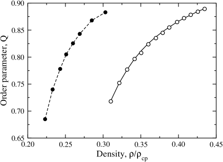
Figure 1: Order parameter $Q$ as a function of the density (measured far from the surface). The density is expressed relative to the closed-packed density $\rho_{\text{cp}}$ for perfectly aligned ellipsoids. Filled circles: simulation results. Open circles: Onsager theory calculations in slab geometry. Solid line: Onsager theory, bulk.

The Onsager theory does not describe the bulk equation for the state perfectly: the predicted bulk density for a given order parameter value is larger than the value obtained in the simulation.

With this choice, the same values of the chemical potential and the same slab dimensions, minimization of the grand potential was carried out for the system with an external field applied near the right wall. Profiles of director angle $\theta(z)$ are compared with elastic theory (eqn (8)) in Fig. 2.

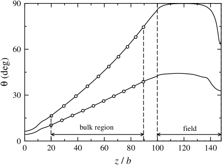
Figure 2: Typical profiles of director angle $\theta(z)$ in the slab geometry. Orienting fields are applied in the region $100<z/b<148$ near the right wall, favouring director angles of $\pi/4$ and $\pi/2$ relative to the surface normal. The left wall is unperturbed. Solids lines: Onsager theory. Circles: results of fitting the profiles in the bulk region with the prediction of elastic theory.

The elastic theory has been fitted to the director angle profiles predicted by the Onsager theory using two adjustable parameters, the extrapolation length $\lambda$ and the elastic constant ratio $\delta$. Note that only part of the bulk region has been used for fitting, $20<z/b<80$ where the elastic theory is applicable.

The anisotropy of elastic constants $\delta$ obtained from fitting is shown in Fig. 3, together with the results of calculations using the Poniewierski and Stecki expressions.

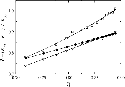
Figure 3: Ratio of the elastic constants, $\delta=(K_{33}-K_{11})/K_{33}$. Circles: Poniewierski - Stecki expressions. Squares: Onsager theory in slab geometry, with wall anchoring field at angle $\alpha=\pi/4$, fitted with the results of elastic theory. Triangles: Onsager theory with $\alpha=\pi/2$, fitted with elastic theory.

The value of $\delta$, and hence the splay constant $K_{1}$, comes into play only as the deformation angle $\theta(z)$ increases. Therefore, for the external field with easy axis $\theta_{L}=\pi/4$, the error in the determination of $\delta$ from simulation data is quite large.

The dependence of the extrapolation length, $\lambda$, on the order parameter $Q$ is shown in Fig 4. It is seen that Onsager theory predicts the extrapolation length to grow linearly with the order parameter, which is completely different from the experimental results in thermotropic liquid crystals, where $\lambda$ decreases with the increase of the order parameter as $Q^{-2}$.

We have also carried out minimization of the grand potential for the system without an external field. As a result, we obtained the single-particle density with a homeotropic distribution of the director in the cell. The dependence of the extrapolation length on the order parameter was then calculated using eqn (41) and is also shown in Fig 4. The results qualitatively agree with the results of fitting obtained by combining Onsager theory and elastic theory. The extrapolation length tends to grow with increase in the order parameter and has the same order of magnitude. Plugging this single-particle density into all equations preceding eqn (41) we were able to check the approximations we did deriving this equation. We found that the most crude approximation is the truncation of the sum in eqn (40). This is not a fundamental problem and can be easily corrected by taking into account a sufficient number of expansion coefficients. However, this points out that the dependence of the director on the $z$ coordinate near the cell surface is different from the linear dependence in the cell bulk. Moreover, to obtain correct quantitative values of the anchoring coefficient, or extrapolation length, one needs to know the director distribution at the surface. The assumption $\delta\bm{n}=\text{const}$ in the interface region, which has been made in Stelzer et al. (1997), may lead to absolutely incorrect estimates of the anchoring coefficient.

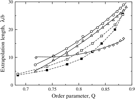
Figure 4: Extrapolation length $\lambda$ as a function of the order parameter. Circles: Onsager theory in slab geometry, director profiles fitted with elastic theory, for anchoring field with $\alpha=\pi/4$. Triangles: the same, but for $\alpha=\pi/2$. Diamonds: Onsager theory in slab geometry, with no field, extrapolation length calculated using equation (41). Filled squares: Monte Carlo results obtained by measuring director fluctuations. Open squares: Monte Carlo results, with applied field near the right-hand wall.

VI.3 Simulation

Simulations were carried out in slab geometry for several values of the number density. The density variation $0.25\leq\rho/\rho_{\text{cp}}\leq 0.34$ provides a sufficient range of order parameter variation in the nematic phase, $0.68\leq Q\leq 0.88$ for us to study the effect of ordering on elastic behaviour.

The order tensor fluctuations in reciprocal space were calculated using expression (48). To fit the simulation results we used expression (49). Recall that the size of the simulation box $L_{z}$ is not necessarily equal to the liquid crystal cell thickness $L$ appearing in the elastic theory. We found that $L=L_{z}+2L_{\text{w}}$, with $L_{\text{w}}\approx 4.5b=0.3a$, almost independent of the density.

Using this value of $L_{\text{w}}$ we adjusted the extrapolation length $\lambda$ and the elastic constant $K_{33}$ to obtain the best fit to the fluctuation amplitudes. Typical order fluctuation amplitudes together with the corresponding fitting curves are plotted in Fig 5.

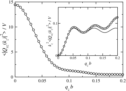
Figure 5: Fluctuations of the director (arbitrary units) as a function of wave-vector (normalized by the molecular minor axis length $b$). Symbols: Monte Carlo results. Solid lines: elastic theory, fitted to parameters discussed in the text. Inset: fluctuations multiplied by $(k_{z}b)^{2}$ to emphasize structure at higher wave numbers.

From this plot one can see that the fitting curves agree quite well with the simulation results for small values of the wave-vector $k_{z}$. At higher $k_{z}$, the structure is not perfectly reproduced, as one would expect for a theory valid for long-wavelength fluctuations, but the agreement is satisfactory.

The elastic constant, $K_{33}b/k_{\text{B}}T$ versus order parameter $Q$ is plotted in Fig 6. The agreement with the Onsager theory is satisfactory, especially if we take into account that the equation of state is not perfectly reproduced by the Onsager theory.

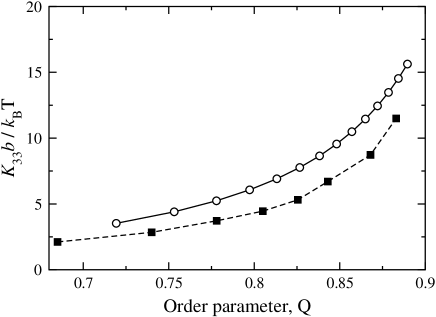
Figure 6: $K_{33}b/k_{\text{B}}T$. Circles: Onsager bulk calculations. Squares: MC simulation results.

The dependence of the extrapolation length, $\lambda$, on the order parameter $Q$ is shown in Fig 4, together with the results from the Onsager theory. It should be noted that combining the elastic approach with the Onsager calculations does not allow one to determine, separately, $L_{\text{w}}$ and $\lambda$. Therefore, the results of the Onsager theory in Fig 4 really represents $\lambda+L_{\text{w}}$, which is one of the possible origins of the systematic difference between the two approaches.

To double check the results obtained by examining the director fluctuation amplitudes, we performed the same type of experiments as in the Onsager slab system. Within a range $7.5b$ of the right-hand wall, a strong coupling field was applied to molecular orientations, $V^{\text{ext}}\sim(\bm{u}_{i}\cdot\bm{e}_{z})^{2}$, aligning the molecules near the right wall parallel to it. After the system was equilibrated, the director profile was fitted to the result of the elastic theory, eqn (8). The dependence of the extrapolation length $\lambda$ on the order parameter $Q$ is also shown in Fig 4. One can see that the agreement between the two methods is quite good.

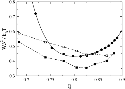
Figure 7: Anchoring energy $W$ as a function of the order parameter. Circles: Onsager theory (with a smooth curve to guide the eye). Open squares: MC results obtained by measuring director fluctuations. Filled squares: MC results, field near the right-hand wall.

Finally, we plot the dependence of the anchoring energy coefficient, $W=K_{33}/\lambda$, which is an intrinsic charachteristic of the interface region, in Fig. 7. For Onsager theory, $\lambda(Q)$ is given by the results in slab geometry fitted with the elastic theory (Fig. 4), $K_{33}(Q)$ - by the Poniewierski - Stecki expressions (Fig. 6). For MC simulations, we used the elastic constant obtained from the analysis of the director fluctuation amplitudes. All methods predict that the anchoring coefficient is a non-monotonic function of the order parameter, even though the actual variation is small.

VII Conclusions

We have studied the dependence of the zenithal surface anchoring coefficient on the order parameter of a lyotropic nematic liquid crystal modeled by hard ellipsoids. Several techniques have been used: Onsager theory combined with elastic theory; Monte Carlo simulations fitted to elastic theory; analysis of the director fluctuation amplitudes obtained from Monte Carlo simulations. The results of these methods agreed qualitatively with each other.

Perhaps the most interesting aspect of this study is the increase of the anchoring extrapolation length with the increase of the nematic order parameter. This implies that the bulk elastic moduli in our system grow faster than the surface anchoring strength. This is opposite to the experimentally observed behaviour in thermotropic nematics, where the extrapolation length goes down with increase of the order parameter.

A microscopic semi-qualitative expression for the extrapolation length allowed us to conclude that subsurface variations of the single-particle density, mainly defined by the nematic order parameter and density variation, contribute substantially to the anchoring phenomenon. We showed that for an ideal system, in which the single-particle density in the cell is assumed to be uniform, the extrapolation length does not depend on the nematic order parameter. This dependence is therefore associated with the subsurface variations of the single-particle density.

We now turn to a brief discussion about possible generalizations of this work. First, it would be interesting to go beyond the limits of Onsager theory and use the direct pair correlation function in the nematic liquid instead of the Mayer $f$-function. Second, as was shown in sec. III.4, the anchoring coefficient can be calculated if we know the single-particle density and the direct pair correlation function (or Mayer $f$-function in case of Onsager theory). This has also been done by Stelzer et al Stelzer et al. (1997) with numerous approximations. Combining elastic theory and local density functional theory one can avoid these approximations, or at least check their validity. This work is in progress.

Appendix A Elastic constants

Performing the integrations over the angles in expression (23) and making use of the properties of $3j$ symbols and spherical harmonics one obtains

$$\beta K_{11} = \kappa(1,1,1,1,1,1),$$ (50)

$$\beta K_{22} = \kappa(1,-1,1,-1,1,-1),$$

$$\beta K_{33} = \kappa(-2,0,-2,0,-2,0),$$

where

$$\kappa(b_{1},b_{2},b_{3},b_{4},b_{5},b_{6})=$$ (67)

$$\frac{4\pi^{2}}{3}\sum_{\ell}^{\text{even}}\ell(\ell+1)\rho_{\ell}^{2}\left[-\left(\begin{array}[]{ccc}\ell&\ell&0\\ 1&-1&0\end{array}\right)I^{\ell,\ell,0}+\frac{b_{1}}{5}\left(\begin{array}[]{ccc}\ell&\ell&2\\ 1&-1&0\end{array}\right)I^{\ell,\ell,2}+\frac{b_{2}}{5}\sqrt{\frac{3}{2}}\left(\begin{array}[]{ccc}\ell&\ell&2\\ 1&1&-2\end{array}\right)I^{\ell,\ell,2}\right]+$$

$$\sqrt{\frac{(\ell+1)!}{(\ell-3)!}}\rho_{\ell}\rho_{\ell-2}\left[\frac{b_{3}}{5}\left(\begin{array}[]{ccc}\ell&\ell-2&2\\ 1&-1&0\end{array}\right)+\frac{b_{4}}{5}\sqrt{\frac{3}{2}}\left(\begin{array}[]{ccc}\ell&\ell-2&2\\ 1&1&-2\end{array}\right)\right]I^{\ell,\ell-2,2}+$$

$$\sqrt{\frac{(\ell+3)!}{(\ell-1)!}}\rho_{\ell}\rho_{\ell+2}\left[\frac{b_{5}}{5}\left(\begin{array}[]{ccc}\ell&\ell+2&2\\ 1&-1&0\end{array}\right)+\frac{b_{6}}{5}\sqrt{\frac{3}{2}}\left(\begin{array}[]{ccc}\ell&\ell+2&2\\ 1&1&-2\end{array}\right)\right]I^{\ell,\ell+2,2},$$

and $I^{\ell_{1},\ell_{2},\ell}$ are radial integrals over the expansion coefficients of the Mayer $f$-function

$$I^{\ell_{1},\ell_{2},\ell}=\int drr^{4}f^{\ell_{1},\ell_{2},\ell}(r).$$ (68)

Expression (50) is the same as obtained before by Stelzer et al Stelzer et al. (1995), except that we used $3j$ symbols instead of Clebsch-Gordan coefficients and a different normalization of the single-particle density. To simplify (67) we use the relation between the $3j$ symbols

$$\sqrt{\frac{3}{2}}\left(\begin{array}[]{ccc}\ell&\ell+2&2\\ 1&1&-2\end{array}\right)=\frac{1}{2}\left(\begin{array}[]{ccc}\ell&\ell+2&2\\ 1&-1&0\end{array}\right),$$ (69)

and take into account that sums with $b_{3}$, $b_{5}$ and $b_{4}$, $b_{6}$ are identical, since

$$\left(\begin{array}[]{ccc}\ell_{1}&\ell_{2}&2\\ 1&-1&0\end{array}\right)=(-1)^{\ell_{1}+\ell_{2}}\left(\begin{array}[]{ccc}\ell_{2}&\ell_{1}&2\\ -1&1&0\end{array}\right)=\left(\begin{array}[]{ccc}\ell_{2}&\ell_{1}&2\\ 1&-1&0\end{array}\right),$$

and $I^{\ell_{1},\ell_{2},2}=I^{\ell_{2},\ell_{1},2}$. Performing simplifications and taking into account explicit expressions for the $3j$ coefficients Edmonds (1974) we obtain expression (24).

Appendix B Expansion of the kernel

From the numerical data we found that the kernel of the integral equation $A_{221}(z)$ can be accurately approximated with a Gaussian function

$$A_{2,2,1}(z)=-\frac{V_{22}}{4\pi\sqrt{\pi}l}\exp\left[-(z/l)^{2}\right],$$ (70)

where we took into account that $-4\pi\int_{-\infty}^{\infty}A_{2,2,1}(z)dz=V_{22}$. Here $l$ is a geometrical parameter which depends only on the elongation of the molecules.

Using the generating function for the Hermite polynomials Gradshtein and Ryzhik (1994)

$$\exp(-t^{2}+2tx)=\sum_{n=0}^{\infty}H_{n}(x)\frac{t^{n}}{n!}$$ (71)

one can write the kernel in a separable form

$$A_{2,2,1}(z_{2}-z_{1})=-\frac{V_{22}}{4\pi\sqrt{\pi}l}\exp\left[-(z_{2}/l)^{2}\right]\times$$

$$\sum_{n=0}^{\infty}\frac{1}{n!}\left(\frac{z_{1}}{l}\right)^{n}H_{n}\left(z_{2}/l\right),$$ (72)

similar to the general case we used in sec. III.4.

Using this approximation to the kernel one can show that the expression for the anchoring coefficient (42) reads

$$\lambda=l/\sqrt{\pi}.$$ (73)

For ellipsoids with elongation $e=15$, we found $l\approx 5.46b$. This results in an anchoring coefficient $\lambda\approx 3.1b$ which is much lower than the actual value of the anchoring in the system with the density and order parameter variations at the surfaces. Hence, changes in the density, order parameter, and, as a result, in the director profile in the interface region cannot be neglected (see also sec. VI.2).

References

- de Gennes and Prost (1995) P. G. de Gennes and J. Prost, The Physics of Liquid Crystals (Clarendon Press, Oxford, 1995), second, paperback ed.
- Rapini and Papoular (1969) A. Rapini and M. Papoular, J. de Physique Colloque 30, C4 (1969).
- Subacius et al. (1995) D. Subacius, V. M. Pergamenshchik, and O. D. Lavrentovich, Appl. Phys. Lett. 67, 214 (1995).
- Yokoyama and van Sprang (1985) H. Yokoyama and H. A. van Sprang, J. Appl. Phys. 57, 4520 (1985).
- Nastishin et al. (1999) Y. A. Nastishin, R. D. Polak, S. V. Shiyanovskii, V. H. Bodnar, and O. D. Lavrentovich, J. Appl. Phys. 86, 4199 (1999).
- Mertelj and Čopič (2000) A. Mertelj and M. Čopič, Phys. Rev. E 61, 1622 (2000).
- Tjipto-Margo and Sullivan (1988) B. Tjipto-Margo and D. Sullivan, J. Chem. Phys. 88, 6620 (1988).
- Teixeira et al. (2001) P. I. C. Teixeira, A. Chrzanowska, G. D. Wall, and D. J. Cleaver, Molec. Phys. 99, 889 (2001).
- Stelzer et al. (1997) J. Stelzer, L. Longa, and H. R. Trebin, Phys. Rev. E 55, 7085 (1997).
- Phuong et al. (2001) N. H. Phuong, G. Germano, and F. Schmid, J. Chem. Phys. 115, 7227 (2001).
- Skačej et al. (1997) G. Skačej, V. M. Pergamenshchik, A. L. Alexe-Ionescu, G. Barbero, and S. Žumer, Phys. Rev. E 56, 571 (1997).
- Priezjev and Pelcovits (2000) N. Priezjev and R. A. Pelcovits, Phys. Rev. E 62, 6734 (2000).
- Onsager (1949) L. Onsager, Ann. N. Y. Acad. Sci. 51, 627 (1949).
- Evans (1992) R. Evans, in Fundamentals of Inhomogeneous Fluids, edited by D. Henderson (Dekker, New York, 1992), chap. 3, pp. 85–175.
- Gray and Gubbins (1984) C. G. Gray and K. E. Gubbins, Theory of molecular fluids. 1. Fundamentals (Clarendon Press, Oxford, 1984).
- Press et al. (1992) W. H. Press, B. P. Flannery, S. A. Teukolsky, and W. T. Vetterling, Numerical Recipes in Fortran (Cambridge University Press, Cambridge, 1992), 2nd ed.
- Poniewierski and Stecki (1979) A. Poniewierski and J. Stecki, Molec. Phys. 38, 1931 (1979).
- Lipkin et al. (1985) M. D. Lipkin, S. A. Rice, and U. Mohanty, J. Chem. Phys. 82, 472 (1985).
- Yokoyama (1997) H. Yokoyama, Phys. Rev. E 55, 2938 (1997).
- Stelzer et al. (1995) J. Stelzer, L. Longa, and H. R. Trebin, J. Chem. Phys. 103, 3098 (1995).
- Somoza and Tarazona (1991) A. M. Somoza and P. Tarazona, Molec. Phys. 72, 911 (1991).
- Andrienko et al. (2000) D. Andrienko, G. Germano, and M. P. Allen, Phys. Rev. E 62, 6688 (2000).
- Allen and Frenkel (1988) M. P. Allen and D. Frenkel, Phys. Rev. A 37, 1813 (1988).
- Allen and Frenkel (1990) M. P. Allen and D. Frenkel, Phys. Rev. A 42, 3641 (1990), erratum.
- Allen (1999) M. P. Allen, Molec. Phys. 96, 1391 (1999).
- Forster (1975) D. Forster, Hydrodynamic Fluctuations, Broken Symmetry and Correlation Functions, vol. 47 of Frontiers in Physics (Benjamin, Reading, 1975).
- Frenkel et al. (1984) D. Frenkel, B. M. Mulder, and J. P. McTague, Phys. Rev. Lett. 52, 287 (1984).
- Frenkel and Mulder (1985) D. Frenkel and B. M. Mulder, Molec. Phys. 55, 1171 (1985).
- Tjipto-Margo et al. (1992) B. Tjipto-Margo, G. T. Evans, M. P. Allen, and D. Frenkel, J. Phys. Chem. 96, 3942 (1992).
- Allen (1993) M. P. Allen, Phil. Trans. Roy. Soc. A 344, 323 (1993), theme Issue: Understanding Self-assembly and Organization in Liquid Crystals.
- Allen et al. (1993) M. P. Allen, G. T. Evans, D. Frenkel, and B. Mulder, Adv. Chem. Phys. 86, 1 (1993).
- Edmonds (1974) A. R. Edmonds, Angular momentum in quantum mechanics (Princeton University Press, Princeton, New Jersey, 1974).
- Gradshtein and Ryzhik (1994) I. S. Gradshtein and I. M. Ryzhik, Tables of integrals, series and products (Academic Press, Boston, 1994).