Hartree-Fock-LAPW method: using the full potential treatment for exchange

Abstract

We formulate a Hartree-Fock-LAPW method for electronic band structure calculations. The method is based on the Hartree-Fock-Roothaan approach for solids with extended electron states and closed core shells where the basis functions of itinerant electrons are linear augmented plane waves. All interactions within the restricted Hartree-Fock approach are analyzed and in principle can be taken into account. In particular, we have obtained the matrix elements for the exchange interactions of extended states and the crystal electric field effects. In order to calculate the matrix elements of exchange for extended states we first introduce an auxiliary potential and then integrate it with an effective charge density corresponding to the electron exchange transition under consideration. The problem of finding the auxiliary potential is solved by using the strategy of the full potential LAPW approach, which is based on the general solution of periodic Poisson’s equation. Here we use an original technique for the general solution of periodic Poisson’s equation and multipole expansions of electron densities. We apply the technique to obtain periodic potentials of the face centered cubic lattice and discuss its accuracy and convergence in comparison with other methods.

I Introduction

In contrast to successful applications of the Hartree-Fock (HF) method to molecules, which have become a routine procedure, Hartree-Fock calculations of electron band structure of solids are relatively rare. The electronic band structure calculations mainly rely on the density functional approach [2, 3] with the local density approximation (LDA) or other non-local exchange approximations [4] which try to mimic the Fock exchange for conduction electrons. As known, LD approximation is a product of the Hartree-Fock theory of the free electron gas and as such it inherits its shortcomings. [5] The LD approximation being universal and simple from one side, is structureless and leads to an unphysical self-interaction, [6] from the other. In addition, LDA is an uncontrolled approximation, and there is no straightforward path to further improvements in its accuracy. [3] Therefore, it is highly desirable to combine the Hartree-Fock approach with methods based on plane wave basis sets which traditionally play an important role in the field of electron band structure calculations. Although a variety of computational procedures on periodic HF method has been reported in the literature, [7, 8, 9, 10, 11, 12, 13, 14] all of them use Gaussian-type orbitals (GTO). In this paper we present a merger of the Hartree-Fock approach with the linear augmented plane wave [15, 16, 17] (LAPW) method, which constitutes a new Hartree-Fock-LAPW procedure for electron band structure calculations. The consideration of the LAPW basis is important since the method has been extensively tested and it is traditionally associated with electronic band structure calculations.

At the center of the Hartree-Fock-Roothaan approach there are calculations of the direct Coulomb and the exchange matrix elements [18] and in the present work we consider thoroughly all cases, including the delocalized and localized states. The advantage is that all expressions for the matrix elements can be found in one source (i.e. this paper), but on the other hand, this has led to numerous formulas and their extensive derivations. While GTOs are popular in calculations of molecular systems and have the advantage of giving easily integrable polycentric functions, we lose this benefit working with the LAPW basis set. There, we have to rely on a different strategy of calculations. Our choice here is the full potential LAPW (FP-LAPW) treatment, [19, 20] which is based on the procedure of finding the general solution for a periodic Poisson’s equation. For Poisson’s equation we use a new original technique (Sec. II). It employs the Ewald method [21, 22] for the potential of the monopole terms and an exact expansion in Fourier series in the interstitial region, with a multipole series expansion of the potential inside the spheres.

A principal new element of our work is to use the strategy of the FP-LAPW method for the calculation of exchange matrix elements between itinerant electrons. Indeed, an exchange matrix element $\langle ab|V^{Coul}|ba\rangle$ ($a$ and $b$ here represent electronic states with the same spin component) can be estimated as a Coulomb self-interaction energy of the charge density distribution $\psi_{b}^{*}(\vec{R})\psi_{a}(\vec{R})$, which appears as a result of the electron transition $a\rightarrow b$. The procedure implies (i) an introduction of an auxiliary potential of the charge density $\psi_{b}^{*}(\vec{R})\psi_{a}(\vec{R})$ and (ii) the integration of the potential with the charge density. Such treatment is rigorous and ensures that all contributions including the long range ones (like the exchange Ewald sums) are carefully considered. It is worth to notice that a simple truncation of the exchange series of other methods excludes such long range effects.

Here we also consider crystal electric field (CEF) effects for the closed shell core electrons. Usually in the full potential LAPW treatment the core electrons are taken in the spherical approximation and the CEF effects are ignored. [17] While the crystal field splittings are small it may be still necessary to include these effects for precise calculations of solids where one compares the stability of different crystalline phases where the energy difference is of the order of 100 K. The present consideration is a generalization of previous works on CEF effects. [23, 24, 25, 26]

For clearness and simplicity in the following we consider only one atom per unit cell. However, the method can be easily generalized for the case of a few atoms. In this paper we consider the core states being completely confined inside the spheres. Various improvements of the method in this respect are also possible, [17] but they are not of fundamental importance and will not be concerned here.

The paper is organized as follows. We start with the general solution of periodic Poisson’s equation, Sec. II. In Sec. III we illustrate how this technique works for the case of a face centered cubic (fcc) crystal. We compare the convergence and accuracy of different approaches. Then we discuss the Hartree-Fock-Roothaan method for solids with extended states, Sec. IV, and calculate the direct Coulomb matrix elements for LAPW basis functions. In Sec. V we present calculations of the matrix elements of exchange, while Sec. VI is reserved for our conclusions.

II General solution of periodic Poisson’s equation

The general solution of Poisson’s equation $V^{Coul}$ for a periodic charge density was demanded by necessity to improve the “muffin-tin” (MT) approximation of LAPW method. [15, 16, 17] LAPW electron band structure calculation procedure with the general potential $V^{tot}(\vec{R})=V^{Coul}(\vec{R})+V^{exc}(\vec{R})$ is referred to as the full potential LAPW (FP-LAPW) method [27] since in principle no shape approximation (except LDA) for the potential is assumed. First full potential calculations have been reported in Refs. [28, 27], and since then they are often used to investigate the electron band structure of solids. These FPLAPW calculations are based on the general solution of Poisson’s equation given by Weinert in Ref. [19]. The basic idea which has been proposed already in Ref. [20] includes two steps: 1) to obtain the potential in the interstices and then 2) to solve the boundary value problem inside a sphere. The point 1) in Ref. [19] represents an alternative to the Ewald method [21, 22] where the true charge inside the spheres is replaced with a pseudo-charge-density of the same multipole moments. In the present paper we propose a new technique which uses the Ewald expansion for the monopoles ($l=0$) and the exact Fourier expansions for the higher multipoles ($l>0$) in the interstitial region. The procedure is straightforward and besides a truncation of the multipole series, it contains only one cut-off parameter for the Ewald expansion. The strategy consists of the same two steps as outlined above. [20, 19]

A Dual and equivalent representations of charge density

We start with the description of charge density in a crystal. For a periodic crystalline structure we introduce $\vec{n}$ to label the sites and the direct lattice vector $\vec{X}(\vec{n})$ which specifies the centers of atoms (spheres). The position vector $\vec{R}$ inside a sphere $S(\vec{n})$ is given by

$$\vec{R}(\vec{n})=\vec{X}(\vec{n})+\vec{r}(\vec{n}).$$ (1)

In spherical coordinates $\vec{r}(\vec{n})=(r(\vec{n}),\hat{r}(\vec{n}))$, where $\hat{r}\equiv\Omega=(\theta,\phi)$. For a Bravais lattice of $\vec{X}(\vec{n})$ we construct the reciprocal lattice of vectors $\vec{K}$. It is convenient to partition the space into the region $S$ inside the non-overlapping spheres of radius $R$ and the interstitial region $I$, Fig. 1.

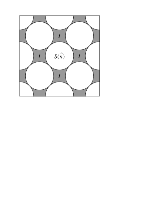
FIG. 1.: The region inside the spheres $S$ (white) and the interstitial region $I$ (gray).

We expand the charge density in Fourier series in region $I$ and in multipolar terms in region $S$ (dual representation [29, 27]):

$$\left.e\rho(\vec{R})\right|_{\vec{R}\in I}=e\sum_{\vec{K}}\rho_{I}(\vec{K})\,e^{i\vec{K}\vec{R}},$$ (3)

$$\left.e\rho(\vec{R})\right|_{\vec{R}\in S}=e\left(\sum_{\Lambda}\rho_{\Lambda}(r)\,S_{\Lambda}(\hat{r})-Z\,\frac{\delta(r)}{\sqrt{4\pi}r^{2}}S_{0}\right).$$ (4)

Angular functions $S_{\Lambda}$ are symmetry adapted functions [30] (SAFs) which are linear combinations of spherical harmonics (see Appendix A for details and definitions). The total density is an invariant of the space group under consideration. Therefore, in the expansion (4) we use only SAFs $S_{\Lambda}$ of the full (or unit) $A_{1g}$ symmetry. Finally, $\delta(r)$ in (4) is the one dimensional (radial) delta-function, $Z$ is the atomic number and $e<0$ is the charge of electron. In the following we will use atomic units and the charge density is understood in units $e=-1$. The density expansion (3,b) called also the dual representation [29, 27] is characteristic of the LAPW method. [15, 16, 17] In fact, the dual representation is natural because in the interstitial region electron density is smooth whereas large charge oscillations near nuclei require a multipole analysis.

Using the linearity of Poisson’s equation we can extend smoothly the interstitial Fourier charge representation inside the spheres and subtract it out. We obtain

$$\rho(\vec{R})=\rho_{I}(\vec{R})+\sum_{S(\vec{n})}\rho^{\prime}_{S(\vec{n})}(\vec{R}),$$ (6)

$$\rho^{\prime}_{S(\vec{n})}(\vec{R})=(\rho_{S(\vec{n})}(\vec{R})-\rho_{I}(\vec{R}))\,\Theta(\vec{R}\in S(\vec{n})),$$ (7)

where $\rho_{I}(\vec{R})$ is defined by (3) over the whole space, $\rho^{\prime}_{S(\vec{n})}$ is the renormalized charge density inside a sphere $S(\vec{n})$ and $\Theta$ is the unit step function. Using Eq. (1) and the plane wave expansion in SAFs centered at the site $\vec{n}$,

$$e^{i\vec{K}\vec{R}}=e^{i\vec{K}\vec{X}(\vec{n})}4\pi\sum_{\Lambda}i^{l}j_{l}(Kr(\vec{n}))S_{\Lambda}(\hat{K})S_{\Lambda}(\hat{r}(\vec{n})),$$ (8)

we rewrite the multipolar density inside the sphere as

$$\rho^{\prime}_{0}(r)=\rho_{0}(r)-\sqrt{4\pi}\rho_{I}(\vec{K}=0)-Z\,\frac{\delta(r)}{\sqrt{4\pi}r^{2}},$$ (10)

$$\rho^{\prime}_{\Lambda}(r)=\rho_{\Lambda}(r)-4\pi i^{l}{\sum_{\vec{K}\neq 0}}^{\prime}j_{l}(Kr)S_{\Lambda}(\hat{K})\rho_{I}(\vec{K}).$$ (11)

We shall refer to (6,b) with the multipole densities (10,b) as to the equivalent representation of the charge density. We will use it every time when we need to obtain the potential in the interstitial region because the Fourier series (3) is now extended to the whole crystal, that has some important advantages (see next subsection).

In principle, in Eq. (3) there is a term with $\vec{K}=0$ that corresponds to the homogeneous electron density distribution. However, it will not contribute to the resulting potential because it cancels with the positive homogeneous density distribution arising from nuclei (see also next subsection).

B The solution in the interstitial region

The potential in the interstices has three components. The first contribution arises from the density $\rho_{I}(\vec{R})$ given by the Fourier series (3) throughout the whole crystal. The second and third terms are due to the monopole ($l=0$) and the high multipole ($l\geq 1$) moments of electron density inside the spheres. (We recall that here we are dealing with the equivalent charge density given by Eqs. (10,b).)

From the Fourier series of $\rho_{I}(\vec{R})$ we find

$$V_{I}(\vec{R})={\sum_{\vec{K}\neq 0}}^{\prime}V^{I}(\vec{K})\,e^{i\vec{K}\vec{R}},$$ (12)

where

$$V^{I}(\vec{K})=\frac{4\pi}{K^{2}}\rho_{I}(\vec{K}).$$ (13)

The easiness of the last expression owes to the fact that we extend the Fourier expansion of $\rho_{I}(\vec{R})$ to the whole crystal. A complication is that the density inside a sphere is renormalized according to Eqs. (10,b). Next we consider a sphere $S(\vec{n})$ and for a moment we will not include to the potential the contribution due to the charges outside the sphere. Thus we introduce a single sphere potential ${\cal U}_{S}(\vec{r})={\cal U}_{S(\vec{n})}(\vec{r}(\vec{n}))$. Using the one-site expansion [31] in SAFs

$$\frac{1}{|\vec{r}(\vec{n})-\vec{r}^{\prime}(\vec{n})|}=\sum_{\Lambda}v_{\Lambda\Lambda}(\vec{n}=\vec{n}^{\prime},r,r^{\prime})S_{\Lambda}(\hat{r}^{\prime})S_{\Lambda}(\hat{r}),$$ (14)

where

$$v_{\Lambda\Lambda^{\prime}}(\vec{n}=\vec{n}^{\prime},r,r^{\prime}) = \int d\Omega\int d\Omega^{\prime}\frac{S_{\Lambda}(\Omega)S_{\Lambda^{\prime}}(\Omega^{\prime})}{|\vec{r}(\vec{n})-\vec{r}^{\prime}(\vec{n})|}$$ (15)

$$= \delta_{\Lambda\Lambda^{\prime}}\frac{4\pi}{2l+1}\frac{r_{<}^{l}}{r_{>}^{l+1}},$$ (16)

and $r_{<}$ ($r_{>}$) is the smaller (larger) of $r$ and $r^{\prime}$, we obtain the solution inside the sphere ($0<r\leq R$),

$${\cal U}_{S}(\vec{r}) = \frac{Q_{0}(r)}{r}+Q^{\prime}_{0}(r)$$ (17)

$$+ {\sum_{\Lambda\neq 0}}^{\prime}\frac{4\pi}{2l+1}\left(\frac{Q_{\Lambda}(r)}{r^{l+1}}+r^{l}Q^{\prime}_{\Lambda}(r)\right)S_{\Lambda}(\hat{r}).$$ (18)

Here we have introduced the functions

$$Q_{0}(r)=q_{0}(r)-\frac{4\pi r^{3}}{3}\rho_{I}(\vec{K}=0),$$ (20)

$$Q^{\prime}_{0}(r)=q^{\prime}_{0}(r)-2\pi(R^{2}-r^{2})\,\rho_{I}(\vec{K}=0),$$ (21)

with

$$q_{0}(r)=\sqrt{4\pi}\int_{0}^{r}\rho_{0}(r^{\prime})\,{r^{\prime}}^{2}dr^{\prime}-Z,$$ (23)

$$q^{\prime}_{0}(r)=\sqrt{4\pi}\int_{r}^{R}\rho_{0}(r^{\prime})\,r^{\prime}dr^{\prime},$$ (24)

for the spherically symmetric term $\Lambda=l=0$, and

$$Q_{\Lambda}(r)=\int_{0}^{r}\rho^{\prime}_{\Lambda}(r^{\prime})\,{r^{\prime}}^{\,l+2}dr^{\prime},$$ (26)

$$Q^{\prime}_{\Lambda}(r)=\int_{r}^{R}\rho^{\prime}_{\Lambda}(r^{\prime})\,{r^{\prime}}^{\,1-l}dr^{\prime},$$ (27)

for the other multipoles, $\Lambda\neq 0$. Taking into account the explicit expression for $\rho^{\prime}(r)$, Eq. (11), we rewrite (26,b) as

$$Q_{\Lambda}(r) = q_{\Lambda}(r)-4\pi i^{l}r^{l+2}{\sum_{\vec{K}\neq 0}}^{\prime}S_{\Lambda}(\hat{K})\rho_{I}(\vec{K})\frac{j_{l+1}(Kr)}{K},$$ (29)

$$Q^{\prime}_{\Lambda}(r) = q^{\prime}_{\Lambda}(r)+4\pi i^{l}{\sum_{\vec{K}\neq 0}}^{\prime}S_{\Lambda}(\hat{K})\rho_{I}(\vec{K})$$ (31)

$$\times \frac{1}{K}\left(\frac{j_{l-1}(KR)}{R^{l-1}}-\frac{j_{l-1}(Kr)}{r^{l-1}}\right),$$ (32)

where

$$q_{\Lambda}(r) = \int_{0}^{r}\rho_{\Lambda}(r^{\prime})\,{r^{\prime}}^{\,l+2}dr^{\prime},$$ (33)

$$q^{\prime}_{\Lambda}(r) = \int_{r}^{R}\rho_{\Lambda}(r^{\prime})\,{r^{\prime}}^{\,1-l}dr^{\prime}.$$ (34)

In order to obtain Eq. (LABEL:2.12a,b) we have performed integration of spherical Bessel functions using the properties 10.1.23, 10.1.24 of Ref. [32].

For the potential ${\cal U}_{S}(\vec{r})$ outside the sphere $S(\vec{n})$ ($r\geq R$) we have

$${\cal U}_{S}(\vec{r})=\frac{Q_{0}(R)}{r}+{\sum_{\Lambda\neq 0}}^{\prime}\frac{4\pi}{2l+1}\frac{Q_{\Lambda}(R)}{r^{l+1}}S_{\Lambda}(\hat{r}).$$ (35)

Now we are ready to compute the potential of the periodic arrangements of the spheres,

$$V_{S}(\vec{R})=\sum_{\vec{n}}{\cal U}_{S}(\vec{R}-\vec{X}(\vec{n})).$$ (36)

Since we seek for the solution in the interstitial region it is desirable to expand it in a Fourier series, in the spirit of the dual representation,

$$V_{S}(\vec{R})={\sum_{\vec{K}\neq 0}}^{\prime}V^{S}(\vec{K})\,e^{i\vec{K}\vec{R}}.$$ (38)

We distinguish two contributions, $V^{S}_{0}$ and $V^{S}_{M}$, from the spherically symmetric charge distribution and from the other higher charge multipoles, respectively:

$$V^{S}(\vec{K})=V^{S}_{0}(\vec{K})+V^{S}_{M}(\vec{K}).$$ (39)

The monopole term ($l=0$) $V^{S}_{0}$ can not be computed directly and requires a special treatment. Here we employ the Ewald method [21, 22] and obtain for the Fourier coefficients

$$V^{S}_{0}(\vec{K})=\frac{\pi}{v}\frac{4}{K^{2}}\,e^{-K^{2}/4G^{2}}Q_{0}(R),$$ (40)

where $G$ is the Ewald cut-off parameter and $v$ is the unit cell volume, $v=V/N$. The improved Ewald technique requires an additional summation in real space, see Ref. [22]. Since we are concerned with the Fourier expansion in the interstitial region we can always take $G$ large enough and neglect the summation in real space. (At large $G$ the dimensionless parameter $c=GR\gg 1$ and the complementary error function decreases exponentially.) Then the Ewald expansion with the Fourier coefficients (40) converges absolutely in the interstitial region.

In the Ewald expansion, Eq. (40), and in the Fourier decomposition (12) we have omitted the terms with $\vec{K}=0$ which correspond to a homogeneous charge distribution of the electrons and the nuclei. Both these terms, considered separately, diverge. Their sum, however, as a consequence of electroneutrality gives the zero value of the charge density and therefore can be discarded.

The high multipole terms ($l\geq 1$) converge fast. Their Fourier coefficients are given by

$$V^{S}_{M}(\vec{K})=\frac{1}{v}\int_{cell}e^{-i\vec{K}\vec{R}}\,V_{S_{M}}(\vec{R})\,d^{3}R.$$ (41)

Here the integration is over any primitive unit cell of the crystal, and $V_{S_{M}}(\vec{R})$ is the potential (36) where only the high multipoles ($l\geq 1$) are retained in ${\cal U}_{S}$. Since the result of integration (41) does not depend on the choice of unit cell, it follows [22] that the coefficients $V^{S}_{M}(\vec{K})$ can be rewritten as

$$V^{S}_{M}(\vec{K})=\frac{1}{v}\int_{crystal}e^{-i\vec{K}\vec{R}}\,{\cal U}_{S_{M}}(\vec{R})\,d^{3}R.$$ (42)

Here the integration is taken over the whole crystal and ${\cal U}_{S_{M}}(\vec{R})$ is given by the last (high multipole) term on the right hand sides of (18) and (35) for $0<|\vec{R}|\leq R$ and $|\vec{R}|>R$, respectively. Using Eq. 10.1.24 of Ref. [32] we find

$$V^{S}_{M}(\vec{K}) = \frac{(4\pi)^{2}}{v}{\sum_{\Lambda\neq 0}}^{\prime}\frac{(-i)^{l}}{2l+1}S_{\Lambda}(\hat{K})$$ (45)

$$\times\left(A_{\Lambda}(K)+Q_{\Lambda}(R)\frac{j_{l-1}(KR)}{KR^{l-1}}\right),$$

where

$$A_{\Lambda}(K)=\int_{0}^{R}\left(\frac{Q_{\Lambda}(r)}{r^{l+1}}+r^{l}Q^{\prime}_{\Lambda}(r)\right)j_{l}(Kr)r^{2}dr.$$ (46)

(Note that at $r\rightarrow 0$, $Q_{\Lambda}\rightarrow r^{l+2}$, $Q^{\prime}_{\Lambda}\rightarrow r^{1-l}$, $j_{l}(Kr)\rightarrow r^{l}$ and the integral (46) does not diverge.)

Collecting all contributions together, Eqs. (13), (40), (45), we obtain for the Coulomb potential in the interstitial region,

$$V(\vec{R}\in I)={\sum_{\vec{K}\neq 0}}^{\prime}V(\vec{K})\,e^{i\vec{K}\vec{R}},$$ (48)

where

$$V(\vec{K})=V^{I}(\vec{K})+V^{S}_{0}(\vec{K})+V^{S}_{M}(\vec{K}).$$ (49)

C The solution inside the spheres

The potential in the form (48,b) can not be extended directly to the region $S$ inside the spheres. The main reason is that it requires an infinite number of plane waves to describe the Coulomb nucleus singularity. In order to obtain a well-behaved solution we expand the total potential $V(\vec{R})$ inside a sphere $S(\vec{n})$ ($r(\vec{n})\leq R$) in a multipole series [20, 19]

$$V(\vec{r}(\vec{n}))=V_{0}(r)+{\sum_{\Lambda\neq 0}}^{\prime}V_{\Lambda}(r)\,S_{\Lambda}(\hat{r}),$$ (50)

The potential $V(\vec{r}(\vec{n}))$ is defined uniquely by boundary conditions. [31] These are of the Dirichlet kind here, since by using the expansion (48) for $V(\vec{R}\in I)$ on the sphere surface, we arrive at

$$V_{0}(R)={\sum_{\vec{K}\neq 0}}^{\prime}j_{0}(KR)V(\vec{K}),$$ (52)

$$V_{\Lambda}(R)=4\pi i^{l}{\sum_{\vec{K}\neq 0}}^{\prime}j_{l}(KR)S_{\Lambda}(\hat{K})V(\vec{K}).$$ (53)

Now inside the sphere $S(\vec{n})$ we have a Dirichlet problem. [19, 31] We solve it by considering the spherical Green’s function expansion, [31] and rewrite the solution (Eqs. (3.126) and (3.114) of Ref. [31]) in the following form:

$$V(\vec{r}(\vec{n}))=U_{S}(\vec{r}(\vec{n}))+V^{out}_{S}(\vec{r}(\vec{n})),$$ (54)

The potential $U_{S}(\vec{r}(\vec{n}))$ is induced by the charge distribution inside the sphere $S(\vec{n})$. Clearly, it is independent of site $\vec{n}$ and we find

$$U_{S}(\vec{r}) = \frac{q_{0}(r)}{r}+q^{\prime}_{0}(r)$$ (55)

$$+ {\sum_{\Lambda\neq 0}}^{\prime}\frac{4\pi}{2l+1}\left(\frac{q_{\Lambda}(r)}{r^{l+1}}+r^{l}q^{\prime}_{\Lambda}(r)\right)S_{\Lambda}(\hat{r}).$$ (56)

Notice that the potential $U_{S}$ differs from ${\cal U}_{S}$, Eq. (35). In (56) we use $q_{\Lambda}$, Eq. (33), and $q^{\prime}_{\Lambda}$, Eq. (34) (not $Q_{\Lambda}$ and $Q^{\prime}_{\Lambda}$!). $q_{\Lambda}$ and $q^{\prime}_{\Lambda}$ correspond to the initial charge density inside the sphere, Eq. (4), rather than the equivalent one, Eqs. (10,b). $V^{out}_{S}(\vec{r})$ is the potential due to the charge situated outside the sphere $S(\vec{n})$,

$$V^{out}_{S}(\vec{r})=V^{out}_{0}(R)+{\sum_{\Lambda\neq 0}}^{\prime}V^{out}_{\Lambda}(R)\left(\frac{r}{R}\right)^{l}S_{\Lambda}(\hat{r}).$$ (57)

Here the constants $V_{0}^{out}\equiv V_{0}^{out}(R)$ and $V_{\Lambda}^{out}\equiv V_{\Lambda}^{out}(R)$ are given by

$$V^{out}_{0} = V_{0}-\frac{q_{0}(R)}{R},$$ (59)

$$V^{out}_{\Lambda} = V_{\Lambda}-\frac{4\pi}{2l+1}\frac{q_{\Lambda}(R)}{R^{l+1}}.$$ (60)

In the following we drop the argument $R$ in the boundary values $V_{0}\equiv V_{0}(R)$ and $V_{\Lambda}\equiv V_{\Lambda}(R)$. Notice that at $\vec{r}=0$ the potential due to the charges outside the sphere $S(\vec{n})$ is given only by $V^{out}_{0}$ since the other contributions ($l\neq 0$) reduce to zero.

Recalling that the Fourier components of the interstitial potential (48,b) consists of three parts, we distinguish the same three contributions on the sphere surface for $V_{0}$ and $V_{\Lambda}$ in Eqs. (52,b):

$$V_{\Lambda}=V_{\Lambda}^{I}+V_{\Lambda}^{S_{0}}+V_{\Lambda}^{S_{M}}.$$ (61)

Here $V_{\Lambda}^{I}$, $V_{\Lambda}^{S_{0}}$ and $V_{\Lambda}^{S_{M}}$ are obtained by using Eqs. (52,b) where instead of $V(\vec{K})$ we substitute $V^{I}(\vec{K})$, $V_{0}^{S}(\vec{K})$ and $V_{M}^{S}(\vec{K})$, respectively. Taking into account (59,b) we can separate the contributions to $V_{\Lambda}^{out}$ into three parts,

$$V_{\Lambda}^{out}=V_{\Lambda,I}^{out}+V_{\Lambda,S_{0}}^{out}+V_{\Lambda,S_{M}}^{out}.$$ (62)

Here $V_{\Lambda,I}^{out}$ is the contribution from the interstitial region, while $V_{\Lambda,S_{0}}^{out}$ and $V_{\Lambda,S_{M}}^{out}$ accounts for the contributions from the monopoles and the higher multipoles from the sites $\vec{n}^{\prime}\neq\vec{n}$, respectively. Explicitly, we obtain

$$V_{\Lambda,I}^{out}=V_{\Lambda}^{I},$$ (64)

$$V_{\Lambda,S_{0}}^{out}=\left\{\begin{array}[]{l l}V_{0}^{S_{0}}-\frac{q_{0}(R)}{R},&\Lambda=0,\\ V_{\Lambda}^{S_{0}},&\Lambda\neq 0,\end{array}\right.$$ (67)

$$V_{\Lambda,S_{M}}^{out}=\left\{\begin{array}[]{l l}V_{0}^{S_{M}},&\Lambda=0,\\ V_{\Lambda}^{S_{M}}-\frac{4\pi}{2l+1}\frac{q_{\Lambda}(R)}{R^{l+1}},&\Lambda\neq 0.\end{array}\right.$$ (70)

The representation of $V(\vec{R})$ given by Eqs. (54) and (62) is convenient because one clearly distinguishes the intra-site part $V_{S}$ from the inter- site ones, $V_{\Lambda,S_{0}}^{out}$, $V_{\Lambda,S_{M}}^{out}$, and $V_{\Lambda,I}^{out}$.

D Comparison with the two-center expansion of the Coulomb potential

It is instructive to compare the results of the previous subsection with the two-center expansion of the Coulomb potential, [23, 24]

$$\frac{1}{|\vec{R}(\vec{n})-\vec{R}^{\prime}(\vec{n}^{\prime})|}$$ (71)

$$=\sum_{\Lambda\Lambda^{\prime}}v_{\Lambda\Lambda^{\prime}}(\vec{n},\vec{n}^{\prime};\,r,r^{\prime})\,S_{\Lambda}(\hat{r}(\vec{n}))\,S_{\Lambda^{\prime}}(\hat{r}^{\prime}(\vec{n}^{\prime})),$$ (72)

where

$$v_{\Lambda\Lambda^{\prime}}(\vec{n},\vec{n}^{\prime};\,r,r^{\prime})\,=\int\!d\Omega(\vec{n})\int\!d\Omega(\vec{n}^{\prime})\,{\frac{S_{\Lambda}(\hat{n})\,S_{\Lambda^{\prime}}(\hat{n}^{\prime})}{|\vec{R}(\vec{n})-\vec{R}^{\prime}(\vec{n}^{\prime})|}}.$$ (73)

(74)

The potential on the sphere surface at a site $\vec{n}$ is found by integrating (72) over $\vec{r}^{\prime}(\vec{n}^{\prime})$ and summing over the spheres $\vec{n}^{\prime}(\neq\vec{n})$:

$$V_{S}^{out}(\Omega)=V_{0}^{out}+{\sum_{\Lambda\neq 0}}^{\prime}(V_{\Lambda,S_{0}}^{out}+V_{\Lambda,S_{M}}^{out})\,S_{\Lambda}(\Omega),$$ (75)

where (compare with Eqs. (67,c))

$$V_{\Lambda,S_{0}}^{out}={\sum_{\vec{n}^{\prime}\neq\vec{n}}}^{\prime}v_{\Lambda\,0}(\vec{n},\vec{n}^{\prime},R),$$ (77)

$$V_{\Lambda,S_{M}}^{out}={\sum_{\vec{n}^{\prime}\neq\vec{n}}}^{\prime}{\sum_{\Lambda^{\prime}\neq 0}}^{\prime}v_{\Lambda\,\Lambda^{\prime}}(\vec{n},\vec{n}^{\prime},R),$$ (78)

and

$$v_{\Lambda\,\Lambda^{\prime}}(\vec{n},\vec{n}^{\prime},R)=\int_{0}^{R}v_{\Lambda\Lambda^{\prime}}(\vec{n},\vec{n}^{\prime};\,R,r^{\prime})\rho^{\prime}_{\Lambda^{\prime}}(r^{\prime})r^{\prime 2}dr^{\prime}.$$ (79)

Since [33]

$$v_{\Lambda\Lambda^{\prime}}(\vec{n},\vec{n}^{\prime};\,r,r^{\prime})\sim\frac{(r)^{l}(r^{\prime})^{l^{\prime}}}{|\vec{X}(\vec{n})-\vec{X}(\vec{n}^{\prime})|^{l+l^{\prime}+1}},$$ (80)

the sums on $\vec{n}^{\prime}$, Eqs. (77,b), converge fast (except for the case $l=l^{\prime}=0$ which is irrelevant here). Practically, it is enough to consider summations over a few neighboring shells.

In many cases (for the cubic symmetry, for example) the whole sum (78) is small in comparison with (77). Eq. (77) then corresponds to the potential calculated with spherical symmetric charge distributions for the neighbors ($i.e.$ $\Lambda^{\prime}=l^{\prime}=0$) and a homogeneous charge distribution in the interstices, Eqs. (10), (20). It follows from (80) that $v_{\Lambda 0}(\vec{n},\vec{n}^{\prime};\,r,r^{\prime})$ does not depend on $r^{\prime}$ which is a dummy argument and

$$v_{\Lambda\,0}(\vec{n},\vec{n}^{\prime},R)=B_{\Lambda}(\vec{n}^{\prime})\,Q_{0}(R)\frac{1}{\sqrt{4\pi}}.$$ (81)

Here $Q_{0}(R)$ is the effective charge inside the sphere given by Eq. (20), and $B_{\Lambda}(\vec{n}^{\prime})=v_{\Lambda 0}(\vec{n},\vec{n}^{\prime};\,R,r^{\prime})$. Combining (77) and (81) with (57), we introduce the potential

$$V^{CEF}(\vec{r})=\frac{Q_{0}(R)}{\sqrt{4\pi}}{\sum_{\Lambda\neq 0}}^{\prime}B_{\Lambda}\left(\frac{r}{R}\right)^{l}S_{\Lambda}(\hat{r}),$$ (83)

where

$$B_{\Lambda}={\sum_{\vec{n}^{\prime}}}^{\prime}B_{\Lambda}(\vec{n}^{\prime}).$$ (84)

The potential $V^{CEF}$ represents the crystal electric field potential (CEF) for localized electrons at site $\vec{n}$ if there are no multipolar couplings with conduction electrons and the electron density in the interstitial region is homogeneous, $V^{I}(\vec{K})=0$. Examples of calculations of $B_{\Lambda}$ for a face centered cubic lattice (fcc) will be given in the next section. In the nearest neighbor approximation one has $B_{\Lambda}=N_{nn}B_{\Lambda}(\vec{n}^{\prime})$, where $\vec{n}^{\prime}$ refers to any of the nearest neighbors and $N_{nn}$ is the number of nearest neighbors. Such CEF potential has been considered in Refs. [23, 25]. A more sophisticated CEF for localized and itinerant electrons will be discussed in Sec. IV.

III Application to the face centered cubic lattice

In this section we apply the technique of Sec. II to test the method and to calculate some important structural constants. As a Bravais lattice we take the face centered cubic (fcc) lattice.

A Periodic Coulomb potential of the monopole ($l=0$) charge density

We first consider the potential of the unit ($q=1$) point charges situated on a face centered cubic lattice. For simplicity we take the cubic lattice constant $a=1$. (The volume of the unit cell is $v=1/4$.) We consider touching spheres on the fcc lattice with the close contact radius $R=\sqrt{2}/4$. As we know from Sec. II, the crystal potential is defined only if the total charge of the unit cell is zero. Therefore, complementary to the positive point charges we must introduce a compensating negative charge density distributed homogeneously in the interstitial region. The total charge confined in the interstitial region of the unit cell must be $q_{I}=-1$ with the density $\rho_{I}=-1/v_{I}=-4/(1-\pi/3\sqrt{2})$.

Using the method of Sec. II we first expand the potential of the interstitial region in Fourier series and then extend it smoothly to the whole crystal, Eqs. (2.17a,b). There are no high multipole moments inside a sphere and from Eq. (45) we find $V_{M}^{S}(\vec{K})=0$. Due to electroneutrality the terms with $\vec{K}=0$ are omitted. Since in the interstitial region there is only one component $\rho_{I}(\vec{K}=0)$ which is different from zero, this results in $V^{I}(\vec{K}\neq 0)=0$. Therefore, the potential in the interstices is given by (48) where the only nonzero contribution to the Fourier component $V(\vec{K})$ is the Ewald contribution $V_{0}^{S}(\vec{K})$, Eq. (40). Notice that for the Ewald expansion we use an effective point charge $Q_{0}\equiv Q_{eff}=q-\rho_{I}4\pi R^{3}/3=1+\pi/(3\sqrt{2}-\pi)$. The renormalization of charges is the price that we have to pay for the extension of the Fourier expansion inside the spheres, Sec. II.

The potential inside a sphere $S(\vec{n})$ then is given by

$$V(\vec{r})=\frac{1}{r}+V_{0}^{out}+V_{04}\left(\frac{r}{R}\right)^{4}K_{4}(\hat{r}) + V_{06}\left(\frac{r}{R}\right)^{6}K_{6}(\hat{r})$$ (86)

$$+...\;.$$

Here we introduce the cubic harmonics $K_{4}(\Omega)$ and $K_{6}(\Omega)$ which are SAFs $S_{l=4,A1g}(\Omega)$ and $S_{l=6,A1g}(\Omega)$, correspondingly, [30, 34] and

$$V_{0}^{out}=V_{0}-\frac{1}{R}.$$ (87)

It is interesting to remark that although we have started with the model of point charges on the fcc lattice, the total crystal potential (86) acquires contributions of the high multipole orders, $l=4,6,8,...$. The constants $V_{0}$, $V_{04}$, $V_{06}$ of the potential are found from the boundary conditions on the sphere surface, Eqs. (52,b). The potential energy of the charges (fcc lattice) is given by

$$E_{fcc}/N=V_{0}^{out}+\frac{1}{2}\langle V_{I}\rangle=-3.9885\;\mbox{ a.u.},$$ (88)

where $\langle V_{I}\rangle$ is the average potential of the interstitial region $I$,

$$\langle V_{I}\rangle=\frac{1}{v_{I}}\int_{I}V(\vec{R})d\vec{R}=\frac{v}{v_{I}}{\sum_{\vec{K}\neq 0}}^{\prime}V(\vec{K}){\cal O}(\vec{K}).$$ (89)

The overlap integral ${\cal O}(\vec{K})$ reads

$${\cal O}(\vec{K})=\delta_{\vec{K}}-\frac{4\pi R^{2}}{v}\frac{j_{1}(KR)}{K}.$$ (90)

Thus $E_{fcc}/N$, Eq. (88), has the meaning of the Madelung constant for the fcc lattice.

The values $V_{0}$, $V_{04}$, $V_{06}$ and $\langle V_{I}\rangle$ are proportional to the effective charge $Q_{eff}\neq 1$. It is convenient to consider the normalized to the unit charge quantities $\tilde{V}_{0}=V_{0}/Q_{eff}$, $\tilde{V}_{04}=V_{04}/Q_{eff}$, $\tilde{V}_{06}=V_{06}/Q_{eff}$ and $\langle\tilde{V}_{I}\rangle=\langle V_{I}\rangle/Q_{eff}$. We study the convergence of $\tilde{V}_{0}$, $\tilde{V}_{04}$, $\tilde{V}_{06}$ and $\langle\tilde{V}_{I}\rangle$ by employing the Ewald method and the technique of Weinert, Ref. [19]. The results are quoted in Tables I and II where the same number of reciprocal vectors $|\vec{K}|<K_{max}$ is used for both approaches.

TABLE I.: Comparison of the Ewald expansion and the method of Ref. 18. $G$ is the Ewald cut-off parameter, $n$ is the parameter of Ref. 18. “Exact” corresponds to the Ewald expansion with $KR\leq 1779$ and $G=780$, with the accuracy of $\approx 10^{-5}$.

	Ewald			Ref. [19]
$K_{max}R$	$G$	$\tilde{V}_{0}$	$\langle\tilde{V}_{I}\rangle$	$n$	$\tilde{V}_{0}$	$\langle\tilde{V}_{I}\rangle$
11.54	7	-0.4545	-0.5607	5	-0.4996	-0.5607
14.74	8	-0.5131	-0.6200	8	-0.5597	-0.6200
28.45	12.5	-0.6288	-0.7359	17	-0.6287	-0.7359
46.33	20	-0.6778	-0.7849	39	-0.6714	-0.7849
68.54	30	-0.6953	-0.8024	62	-0.6849	-0.8024
90.73	40	-0.7014	-0.8085	84	-0.6911	-0.8085
exact	-	-0.70922	-0.81630	-	-0.70922	-0.81630

TABLE II.: Comparison of the Ewald expansion and the method of Ref. 18. $G$ is the Ewald cut-off parameter, $n$ is the parameter of Ref. 18.

	Ewald			Ref. [19]
$K_{max}R$	$G$	$\tilde{V}_{04}$	$\tilde{V}_{06}$	$n$	$\tilde{V}_{04}$	$\tilde{V}_{06}$
11.54	7	-0.18135	-0.14304	5	-0.18233	-0.14600
14.74	8	-0.18186	-0.14459	8	-0.18192	-0.14459
28.45	12.5	-0.18193	-0.14467	17	-0.18192	-0.14466
46.33	20	-0.18192	-0.14466	39	-0.18192	-0.14466
exact	-	-0.18192	-0.14466	-	-0.18192	-0.14466

(Though we did not optimize the convergence of Fourier series by choosing the best $G$ and $n$ for the Ewald and Weinert approaches.) We observe that $\tilde{V}_{06}$ and $\tilde{V}_{04}$ converge faster than $\tilde{V}_{0}$ and $\langle\tilde{V}_{I}\rangle$.

The Ewald method estimates better the monopole terms $\tilde{V}_{0}$ and $\langle\tilde{V}_{I}\rangle$, Table I. In this case it is simple and stable, while Weinert’ procedure requires evaluation of spherical Bessel functions of higher order for each $\vec{K}$.

Both methods give almost the same results for $\tilde{V}_{04}$ and $\tilde{V}_{06}$, Table II. $\tilde{V}_{04}$ and $\tilde{V}_{06}$ can be calculated independently by means of the two-center expansion of Coulomb interaction, which we have considered in Sec. II D. In that case we first calculate $v_{04}(\vec{n},\vec{n}^{\prime})$ and $v_{06}(\vec{n},\vec{n}^{\prime})$, Eq. (74), where $r=r^{\prime}=R$, with $S_{0}=1/\sqrt{4\pi}$ on a first site $\vec{n}$, and the cubic harmonic (SAF) $K_{4}$ or $K_{6}$ on a second site $\vec{n}^{\prime}$. Since the integrals $v_{04}(\vec{n},\vec{n}^{\prime})$ and $v_{06}(\vec{n},\vec{n}^{\prime})$ decrease very fast with the distance $d$ between the two sites ($1/d^{5}$ for $K_{4}$ and $1/d^{7}$ for $K_{6}$), we obtain $\tilde{V}_{04}$ and $\tilde{V}_{06}$ by summing $v_{04}(\vec{n},\vec{n}^{\prime})$ and $v_{06}(\vec{n},\vec{n}^{\prime})$ over all neighbors $\vec{n}^{\prime}$ on the fcc lattice, i.e.

$$\tilde{V}_{0t}=\frac{1}{\sqrt{4\pi}}{\sum_{\vec{n}^{\prime}}}^{\prime}v_{0t}(\vec{n},\vec{n}^{\prime}),$$ (91)

where $t=4$ or 6. The results of such calculations are shown in Tables III and IV.

TABLE III.: Calculation of $\tilde{V}_{04}$ by summation over neighboring shells, $N_{sh}$ is the number of neighbors in the shell, $\vec{n}^{\prime}$ stands for the coordinates of a shell representative, $v_{04}$ is the two-center integral (2.33) for $S_{0}$ and $K_{4}$. “Exact” means summation over 128428 neighbors ($d\leq 12$) on the fcc lattice.

shell	$N_{sh}$	$\vec{n}^{\prime}$	$v_{04}$	$\tilde{V}_{04}$
1	12	$(\frac{1}{2},\frac{1}{2},0)$	-0.070694	-0.23930
2	6	$(1,0,0)$	0.049988	-0.15470
3	24	$(\frac{1}{2},\frac{1}{2},1)$	-0.004535	-0.18540
4	12	$(1,1,0)$	-0.002209	-0.19288
5	24	$(\frac{3}{2},\frac{1}{2},0)$	0.002782	-0.17405
10				-0.18073
20				-0.18283
exact				-0.18191

TABLE IV.: Calculation of $\tilde{V}_{06}$ by summation over neighboring shells, $N_{sh}$ is the number of neighbors in the shell, $\vec{n}^{\prime}$ stands for the coordinates of a shell representative, $v_{06}$ is the two-center integral (2.33) for $S_{0}$ and $K_{6}$. “Exact” means summation over 111956 neighbors ($d\leq 9$) on the fcc lattice.

shell	$N_{sh}$	$\vec{n}^{\prime}$	$v_{06}$	$\tilde{V}_{06}$
1	12	$(\frac{1}{2},\frac{1}{2},0)$	-0.044247	-0.14978
2	6	$(1,0,0)$	0.002407	-0.14571
3	24	$(\frac{1}{2},\frac{1}{2},1)$	0.000299	-0.14368
4	12	$(1,1,0)$	-0.000346	-0.14485
5	24	$(\frac{3}{2},\frac{1}{2},0)$	0.000005	-0.14482
10				-0.14467
20				-0.14467
exact				-0.14466

The convergent values $\tilde{V}_{04}$ and $\tilde{V}_{06}$ perfectly match those obtained by the techniques of Ewald and Weinert, Table II. However, the Ewald and Weinert’ approaches require less computer time and are more efficient than the two-center expansion. Finally, we would like to remark that the calculated in Table II exact values $\tilde{V}_{04}$ and $\tilde{V}_{06}$ can be used for cubic crystal electric field, Eq. (83,b). For an fcc crystal with the cubic lattice constant $a\neq 1$ we have $B_{4}=\sqrt{4\pi}\,\tilde{V}_{04}/a$ and $B_{6}=\sqrt{4\pi}\,\tilde{V}_{06}/a$.

Although we have analyzed both methods at the close contact radius $R=\sqrt{2}/4$ it is also possible to assess the validity of the two methods by decreasing the sphere radius $r\leq R$. Both methods are designed to describe the potential in the interstitial region. They can not approximate the potential correctly in the whole space. Therefore, both of them are expected to fail at a certain small radius, but their departure from the exact solution is an indication of their accuracy. The results for $\tilde{V}_{04}(r)$ and $\tilde{V}_{06}(r)$ ($K_{max}R$=90.73, $G$=40, $n$=84) at $r<R$ are shown in Fig. 2 and 3.

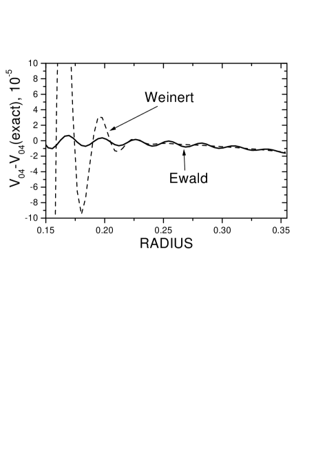
FIG. 2.: Comparison between the Ewald expansion and the method of Ref. 18 for $V_{04}(r)$.

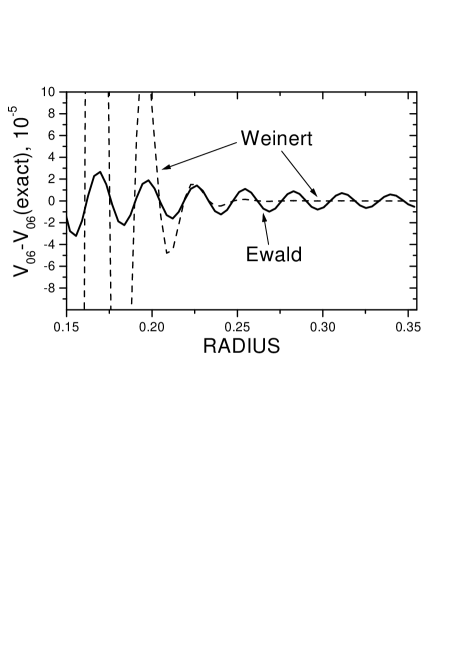
FIG. 3.: Comparison between the Ewald expansion and the method of Ref. 18 for $V_{06}(r)$.

Weinert’ procedure gives more smooth values for $r$ close to $R$, but the Ewald expansion is more stable in the whole range. The calculation of the monopole term $V_{0}^{out}$ (or $V_{0}$) is of special interest. By decreasing the sphere radius $r$ we change the density of the compensating negative charge distribution. As a result, both $V_{0}(r)$ and $V_{0}^{out}(r)$, Eq. (87), are functions of $r$. From the last value however it is possible to reconstruct $V_{0}^{out}(R)$ at the close contact radius $R$. On can easily obtain the result from electrostatic considerations:

$$\left.V_{0}^{out}(R)\right|_{r}=\frac{V_{0}^{out}(r)+2\pi(R^{2}-r^{2})\rho}{1-\frac{4}{3}\pi(R^{3}-r^{3})\rho},$$ (93)

where

$$\rho=\left(\frac{1}{4}-\frac{4\pi}{3}r^{3}\right)^{-1},$$ (94)

In principle, $V_{0}^{out}(R)$ should be independent of $r$, but in practice it exhibits such dependence as indicated on the left hand side of (93). This is because the estimation (93) depends on the accuracy of the calculated value $V_{0}^{out}(r)$ and as such, it is a function of $r$. We find it convenient to study $V_{0}^{out}(R)|_{r}$ which is expected to be constant rather than the initial value $V_{0}^{out}(r)$. In order to compare the two techniques we plot the function $\triangle(r)=(V_{0}^{out}|_{r}-V_{0}^{out}|_{ex})/V_{0}^{out}|_{ex}$ in Fig. 4. ($V_{0}^{out}|_{ex}=-5.5612$ is the best value for $V_{0}^{out}$ calculated from data of Table I, last row.) As one clearly sees from Fig. 4, the Ewald expansion performs better than the approach of Weinert.

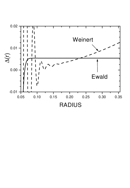
FIG. 4.: Comparison between the Ewald expansion ($G=40$, $KR<90.73$) and the method of Ref. 18 for $V_{0}(r)$ ($n=84$), see text for details.

B Periodic Coulomb potentials of the $l=4$ and $l=6$ cubic charge density

Here we illustrate how the proposed method works for high order multipoles with $l=4$ and $l=6$. We consider two cases. In the first case the charge distribution on the touching sphere surfaces is given by

$$\rho_{4}(\vec{r})=\frac{\delta(r-R)}{r^{2}}\,K_{4}(\hat{r}),$$ (96)

In the second case it is

$$\rho_{6}(\vec{r})=\frac{\delta(r-R)}{r^{2}}\,K_{6}(\hat{r}).$$ (97)

Here $\delta(r^{\prime})$ is the one-dimensional delta-function and $K_{4}$, $K_{6}$ are cubic harmonics (SAFs). [34] Now it is not necessary to introduce a compensating charge in the interstitial region since the total charge of the unit cell given by integration of (96) or (97) over the polar angles yields zero. According to the treatment of Sec. II we start with the potential of a single sphere, say $S(\vec{n}=0)$. The potentials then are

$$U_{S}^{4}(\vec{r})=\frac{4\pi}{9}\frac{1}{R}\left(\frac{r}{R}\right)^{4}K_{4}(\hat{r}),$$ (99)

$$U_{S}^{6}(\vec{r})=\frac{4\pi}{13}\frac{1}{R}\left(\frac{r}{R}\right)^{6}K_{6}(\hat{r}),$$ (100)

for $r\leq R$, and

$$U_{S}^{4}(\vec{r})=\frac{4\pi}{9}\frac{1}{R}\left(\frac{R}{r}\right)^{5}K_{4}(\hat{r}),$$ (102)

$$U_{S}^{6}(\vec{r})=\frac{4\pi}{13}\frac{1}{R}\left(\frac{R}{r}\right)^{7}K_{6}(\hat{r}),$$ (103)

for $r\geq R$. Notice that the potentials $U_{S}^{4}$ and $U_{S}^{6}$ have discontinuous derivatives at $R$. (Here we do not make any distinction between $U(r)$ and ${\cal U}(r)$, Sec. II, since there is no renormalization of the charge density inside a sphere.) Using the method of Sec. II we find from Eqs. (45,b) the Fourier transforms of the potentials of the periodic arrangements of such charged surfaces on the fcc lattice,

$$V_{4}(\vec{K})=\frac{(4\pi)^{2}}{9\,v}\frac{R}{K}(j_{3}(KR)+j_{5}(KR))\,K_{4}(\vec{K}),$$ (105)

$$V_{6}(\vec{K})=-\frac{(4\pi)^{2}}{13\,v}\frac{R}{K}(j_{5}(KR)+j_{7}(KR))\,K_{6}(\vec{K}).$$ (106)

Notice, that we arrive at the same results if first we Fourier transform the densities,

$$\rho_{4}(\vec{K})=\frac{4\pi}{v}j_{4}(KR)\,K_{4}(\vec{K}),$$ (108)

$$\rho_{6}(\vec{K})=-\frac{4\pi}{v}j_{6}(KR)\,K_{6}(\vec{K}),$$ (109)

and then calculate the potentials by means of

$$V_{4}(\vec{K})=\frac{4\pi}{K^{2}}\rho_{4}(\vec{K}),$$ (111)

$$V_{6}(\vec{K})=\frac{4\pi}{K^{2}}\rho_{6}(\vec{K}).$$ (112)

(In oder to establish the equality with (105,b) we used the property 10.1.21 of Bessel functions, Ref. [32].) As we have many times mentioned before (Sec. II) the Fourier expansion is valid only in the interstitial region.

Inside a sphere $S(\vec{n})$ the first potential is given by

$$V_{4}(\vec{r})=V_{40}+V_{44}\left(\frac{r}{R}\right)^{4}K_{4}(\hat{r})+V_{46}\left(\frac{r}{R}\right)^{6}K_{6}(\hat{r})+....$$ (113)

(114)

For the second potential, accordingly, we have

$$V_{6}(\vec{r})=V_{60}+V_{64}\left(\frac{r}{R}\right)^{4}K_{4}(\hat{r})+V_{66}\left(\frac{r}{R}\right)^{6}K_{6}(\hat{r})+....$$ (115)

(116)

The constants $V_{40}$, $V_{60}$, and $V_{44}$, $V_{46}$, $V_{64}$, $V_{66}$ are found from the boundary conditions, Eqs. (52) and (53), where $V(\vec{K})$ is given by $V_{4}(\vec{K})$, Eq. (105), for the first potential and by $V_{6}(\vec{K})$, Eq. (106), for the second potential. (Compare these results with the potentials (99) and (100) for a single sphere.)

In order to distinguish the potential due to the multipole moment of the sphere $S(\vec{n})$ from the potential of the rest of the crystal, we subtract from $V_{4}$ and $V_{6}$ the contribution induced by the multipole moment of the sphere (see Eqs. (64-c)) and introduce the parameters

$$V_{44}^{out}=V_{44}-\frac{4\pi}{9}\frac{1}{R},$$ (118)

$$V_{66}^{out}=V_{66}-\frac{4\pi}{13}\frac{1}{R}.$$ (119)

We have calculated $V_{44}^{out}$, $V_{66}^{out}$, $V_{46}$ and $V_{60}$ and then compared them with those obtained by the method of Ref. [19], see Tables V and VI.

TABLE V.: Comparison of the direct Fourier expansion and the method of Ref. 18. $n_{4}$ and $n_{6}$ are the parameters of Ref. 18 for $V_{4}$ and $V_{6}$. “Exact” corresponds to Weinert’ expansion with $K_{max}R\leq 124.08$ and $n_{4}=96$, $n_{6}=94$.

	direct expansion		Ref. [19]
$K_{max}R$	$V_{44}^{out}$	$V_{66}^{out}$	$n_{4}$	$V_{44}^{out}$	$n_{6}$	$V_{66}^{out}$
35.19	1.8876	1.1750	24	2.2139	22	1.5161
57.37	2.0113	1.3074	46	2.2139	44	1.5334
79.60	2.0688	1.3696	69	2.2140	67	1.5220
101.8	2.1007	1.4036	91	2.2140	89	1.5211
exact	2.21402	1.52112	$-$	2.21402	$-$	1.52112

TABLE VI.: Comparison of the direct Fourier expansion and the method of Ref. 18. $n_{4}$ and $n_{6}$ are the parameters of Ref. 18 for $V_{4}$ and $V_{6}$. “Exact” corresponds to Weinert’ expansion with $K_{max}R\leq 124.08$ and $n_{4}=96$, $n_{6}=94$.

	direct expansion		Ref. [19]
$K_{max}R$	$V_{46}\cdot 10^{2}$	$V_{60}$	$n_{4}$	$V_{46}\cdot 10^{2}$	$n_{6}$	$V_{60}$
35.19	-2.5778	-0.1426	24	-1.6667	22	-0.1442
57.37	-1.9364	-0.1431	46	-1.7042	44	-0.1464
79.60	-1.7908	-0.1436	69	-1.6820	67	-0.1448
101.8	-1.7529	-0.1439	91	-1.6812	89	-0.14467
exact	-1.68119	-0.14466	$-$	-1.68119	$-$	-0.14466

Alternatively, we can compute $V_{44}^{out}$ and $V_{66}^{out}$ by performing the two-center multipole expansions (72), (74). To do it, we first calculate integrals $v_{44}(\vec{n},\vec{n}^{\prime})$ and $v_{66}(\vec{n},\vec{n}^{\prime})$, Eq. (74), between the functions $K_{4}(\vec{n})$ and $K_{4}(\vec{n}^{\prime})$, or between $K_{6}(\vec{n})$ and $K_{6}(\vec{n}^{\prime})$ at sites $\vec{n}$ and $\vec{n}^{\prime}$. By summing over ${\vec{n}^{\prime}}$ on the fcc lattice we estimate $V_{44}^{out}$ and $V_{66}^{out}$, i.e.

$$V_{tt}^{out}={\sum_{\vec{n}^{\prime}}}^{\prime}v_{tt}(\vec{n},\vec{n}^{\prime}),$$ (120)

where $t=4$ or 6. Clearly, the accuracy depends on the number of sites $\vec{n}^{\prime}$ included in the summations. The results of these calculations are given in Table VII. (The representative coordinates of five nearest shells as well as the number of atoms of the shells are quoted in Tab. III.)

TABLE VII.: Calculation of $V_{44}$ and $V_{66}$ by summation over neighboring shells. The discrepancy between the converged value for $V_{66}$ and the exact one from Table VI is due to numerical errors of the two center integration.

shell	$v_{44}$	$V_{44}^{out}$	$v_{66}$	$V_{66}^{out}$
1	0.17897	2.14767	0.12632	1.51593
2	0.01406	2.23204	0.00064	1.51976
3	-0.00091	2.21024	0.00005	1.52088
4	0.00035	2.21444	0.00002	1.52106
5	-0.00002	2.21393	0.0	1.52102
10	$-$	2.21403	$-$	1.52102
20	$-$	2.21401	$-$	1.52102
exact	$-$	2.21402	$-$	1.52112

From the Tables V-VII it follows that the method of Ref. [19] gives a better convergence despite the fact that the expressions (108,b), (111,b) for the Fourier coefficients are exact. Interestingly, the exact expressions formally correspond to $n_{4}=n_{6}=-1$ in Eq. 28 of Ref. [19], while the better convergence is achieved for large positive $n_{4}$ and $n_{6}$ implied by the technique of Ref. [19]. We ascribe this property to the fact that the potentials $V_{4}$ and $V_{6}$ have discontinues derivatives at the sphere boundaries. Therefore, the exact expansions (108,b), (111,b) try to reproduce these cusps while the pseudo-charge density of Ref. [19] has $n-1$ continuous derivatives thereby avoiding the problem. Thus, our test calculations for the densities (96) and (97) indicate that Weinert’ procedure gives a better convergence.

We can also generalize the present consideration for arbitrary multipole sphere moments $Q_{4}(R)$ and $Q_{6}(R)$ given by Eq. (26) on an fcc lattice when its cubic lattice constant $a\neq 1$. For the former case we obtain that the potential inside a sphere due to the other spheres’ multipoles $Q_{4}$ of the fcc crystal is

$$V_{4}^{out}(\vec{r})=B_{40}+B_{44}\left(\frac{r}{R}\right)^{4}K_{4}(\hat{r})+B_{46}\left(\frac{r}{R}\right)^{6}K_{6}(\hat{r})+...,$$ (121)

(122)

where $B_{40}=k_{4}V_{40}$, $B_{44}=k_{4}V_{44}^{out}$, $B_{46}=k_{4}V_{46}$, and the coefficient of proportionality for touching spheres ($R=\sqrt{2}a/4$) is given by

$$k_{4}=\frac{64}{a^{5}}Q_{4}(R).$$ (123)

Analogously, the expression for the potential $V_{6}^{out}$ due to $Q_{6}(R)$ is obtained as

$$V_{6}^{out}(\vec{r})=B_{60}+B_{64}\left(\frac{r}{R}\right)^{4}K_{4}(\hat{r})+B_{66}\left(\frac{r}{R}\right)^{6}K_{6}(\hat{r})+...,$$ (124)

(125)

where $B_{60}=k_{6}V_{40}$, $B_{64}=k_{6}V_{64}$, $B_{66}=k_{6}V_{66}^{out}$, and

$$k_{6}=\frac{512}{a^{7}}Q_{6}(R).$$ (126)

Notice that here we can immediately determine the potentials using exact values $V_{40}=\tilde{V}_{04}$, $V_{44}$, $V_{46}$, $V_{60}=\tilde{V}_{06}$, $V_{64}$ and $V_{66}$ quoted in Tables V and VI. These parameters as well as those calculated in Sec. III.A are in fact important structural constants of the fcc lattice.

IV Hartree-Fock-Roothaan method: Calculations of the direct matrix elements

The Hartree-Fock operator for the electronic system is defined as [18, 7]

$${\cal F}=\sum_{d}\left({\cal H}_{d}+{\cal J}_{d}-{\cal K}_{d}\right),$$ (127)

where ${\cal H}_{d}$ is the Hamiltonian operator for a $d$th electron moving in the field of nuclei alone,

$${\cal H}_{d}=-\frac{\vec{\nabla}^{2}_{d}}{2}-\sum_{\vec{n}}\frac{Z}{|\vec{R}_{d}-\vec{X}(\vec{n})|},$$ (128)

${\cal J}_{d}$ and ${\cal K}_{d}$ are the direct Coulomb and exchange operators, respectively. In order to obtain the best trial function of the $d$th electron, $\psi_{d}(x)=\langle x|d\rangle$, one considers basis functions $\chi_{a}(x)=\langle x|a\rangle$, and expands $\psi_{d}$ in terms of $\chi_{a}$,

$$\psi_{d}(x)=\sum\gamma_{da}\,\chi_{a}(x),$$ (129)

where $\gamma_{da}$ are the coefficients of the expansion, and the index $x$ stands for the coordinates $\vec{R}$ and the spin projection $s_{z}=\pm 1/2$ of the electron, $x\equiv(\vec{R},s_{z})$. For the matrix elements of ${\cal J}_{d}$ and ${\cal K}_{d}$ one has

$$\langle a|{\cal J}_{d}|b\rangle={\sum_{c}}^{\prime}\int\chi_{a}^{*}(x_{1})\chi_{b}(x_{1})\frac{1}{R_{12}}\psi_{c}^{*}(x_{2})\psi_{c}(x_{2})dx_{1}dx_{2},$$ (131)

(132)

$$\langle a|{\cal K}_{d}|b\rangle={\sum_{c}}^{\prime}\int\chi_{a}^{*}(x_{1})\psi_{c}(x_{1})\frac{1}{R_{12}}\chi_{b}(x_{2})\psi_{c}^{*}(x_{2})dx_{1}dx_{2}.$$ (133)

(134)

In Eqs. (132,b) the summation is understood over all occupied electron states except $d$. In the following we consider the restricted HF method. Usually in the HF method [18] the wave function $\psi_{d}(x)=\phi(\vec{R})\zeta(s_{z})$ is given by the coordinate (orbital) part $\phi(\vec{R})$ and the spinor part $\zeta(s_{z})$. However, it is well known that the spin-orbit coupling mixes the two components $\zeta_{+}=\zeta(1/2)$ and $\zeta_{-}=\zeta(-1/2)$. (The spin-orbit coupling is especially important for core shells.) Therefore, here we consider more general spin-orbitals,

$$\psi_{d}(x)=\phi_{+}(\vec{R})\,\zeta_{+}+\phi_{-}(\vec{R})\zeta_{-}.$$ (135)

Using the time reversal symmetry ${\cal T}$, [40] one can construct from $\psi_{d}$ the time reversed state $\psi^{*}_{d}={\cal T}\psi_{d}$ (see Appendix C). According to the Kramers theorem $\psi_{d}$ and $\psi^{*}_{d}$ have the same energy $\epsilon_{d}$ and are orthogonal. Therefore, such treatment is analogous to the conventional restricted HF method [18] with the double occupancy of $\epsilon_{d}$. However, in the following we will treat these two states separately, as different components of a doubled valued irreducible representation. Therefore, although we work within the restricted HF method, there are no factor 2 in front of ${\cal H}_{d}$ and ${\cal J}_{d}$ in Eq. (127). Notice, that as a consequence of (135), the integrals (132,b) include summations over two spin components.

We regroup ${\cal F}$ as

$${\cal F}={\cal F}^{Coul}-{\cal F}^{exc},$$ (136)

where

$${\cal F}^{Coul}=\sum_{d}({\cal H}_{d}+{\cal J}_{d}),$$ (137)

and

$${\cal F}^{exc}=\sum_{d}{\cal K}_{d}.$$ (138)

The matrix elements of ${\cal F}^{Coul}$ can be written in the following form:

$$\langle a|{\cal F}^{Coul}|b\rangle=\int\chi_{a}^{*}(x)\left(-\frac{1}{2}\vec{\nabla}^{2}+V^{d}(\vec{R})\right)\chi_{b}(x)\,dx,$$ (139)

where the Hartree (electrostatic) potential $V^{d}$ acting on the $d$th electron reads

$$V^{d}(\vec{R})={\sum_{c}}^{\prime}\int\frac{\psi_{c}^{*}(x^{\prime})\psi_{c}(x^{\prime})}{|\vec{R}-\vec{R}^{\prime}|}dx^{\prime}-\sum_{\vec{n}}\frac{Z}{|\vec{R}-\vec{X}(\vec{n})|}.$$ (140)

(141)

It is convenient to rewrite the potential as

$$V^{d}(\vec{R})=V(\vec{R})-{\cal V^{\prime}}^{d}(\vec{R}),$$ (142)

where $V(\vec{R})$ is the potential of all electrons and nuclei considered in section II,

$$V(\vec{R})=\int\frac{\rho(\vec{R}^{\prime})}{|\vec{R}-\vec{R}^{\prime}|}d\vec{R}^{\prime},$$ (143)

while ${\cal V^{\prime}}^{d}$ is the potential created by the $d$th electron alone,

$${\cal V^{\prime}}^{d}(\vec{R})=\int\frac{\psi_{d}^{*}(x^{\prime})\psi_{d}(x^{\prime})}{|\vec{R}-\vec{R}^{\prime}|}dx^{\prime}.$$ (144)

The charge density $\rho(\vec{R})$ in (143),

$$\rho(\vec{R})=\rho_{el}(\vec{R})+\rho_{n}(\vec{R}),$$ (146)

comprises the point charges of nuclei,

$$\rho_{n}(\vec{R})=\sum_{\vec{n}}Z\delta(\vec{R}-\vec{X}(\vec{n})),$$ (147)

and the total electronic charge density,

$$\rho_{el}(\vec{R})={\sum_{c}}\psi_{c}^{*}(x)\psi_{c}(x).$$ (148)

(Again, in (148) the summation is implied over two spin components.) In solids we are dealing with the two types of electron states, which are extended states of valence electrons (with the total charge density $\rho_{val}(\vec{R})$) and localized states of core electrons ($\rho_{core}(\vec{r}(\vec{n}))$), and

$$\rho_{el}(\vec{R})=\rho_{val}(\vec{R})+\sum_{\vec{n}}\rho_{core}(\vec{R}-\vec{X}(\vec{n})).$$ (149)

The Hartree-Fock-Roothaan method implies a self-consistent field procedure. [18, 7] In particular, for itinerant states ($d=(\vec{k},\alpha)$) one solves the secular equation

$$\sum_{a}{\cal F}_{ba}(\vec{k},\alpha)\,\gamma_{a}(\vec{k},\alpha)=E(\vec{k},\alpha)\sum_{a}{\cal O}_{ba}(\vec{k})\,\gamma_{a}(\vec{k},\alpha).$$ (150)

(151)

Here $\vec{k}$ is the wave vector, $\alpha$ is the band index, ${\cal O}$ is the overlap matrix and $E(\vec{k},\alpha)$ is the corresponding HF energy. [18] The HF operator ${\cal F}$ depends implicitly on the solution (via the coefficients $\gamma_{a}$). Below in this section we calculate the matrix elements of ${\cal F}^{Coul}$, while in Sec. V we consider the matrix elements of ${\cal F}^{exc}$.

A Multipole expansion of electron density

In order to calculate the matrix elements of ${\cal F}^{Coul}$ for a $d$th electron from Eqs. (139) we have to know the electrostatic potential $V^{d}$, Eq. (141) or (142). We have already thoroughly studied this problem in Sec. II and know how to proceed starting with the dual representation (3,b) of charge density. The only problem is to construct the charge density of the itinerant and the localized electrons. In this subsection we do it explicitly for the core (A1) and the valence (A2) electrons.

A1. The density of the inner closed shells at site ${\vec{n}}$ reads

$$\rho_{core}(\vec{r}(\vec{n}))=\sum_{\tau}n_{\tau}\rho_{\tau}(\vec{r}(\vec{n})),$$ (153)

where

$$\rho_{\tau}(\vec{r})=|\langle\vec{r},s_{z}|\tau\rangle|^{2}=|\langle x|\tau\rangle|^{2}.$$ (154)

Here $\langle x|\tau\rangle$ stands for the wave functions of localized electrons, and $n_{\tau}=1$ if $\epsilon(\tau)<E_{F}$ and zero otherwise ($E_{F}$ is the Fermi energy). In (153) summation over $s_{z}=\pm 1/2$ is implied. Here we will not consider the case of partially filled core shells. (Such situation occurs in lanthanides with localized 4$f$ electrons or in transition elements with $d$ electrons.) Furthermore, we assume that all core electrons at site $\vec{n}$ are confined inside the sphere $S(\vec{n})$ so that the core wave functions with their first derivatives fall to zero at $R$.

The inner closed shells are classified according to the principal quantum number $n$, the total angular momentum (including spin) $j$ and the orbital number $l$. In the case of the spherical symmetry these $(2j+1)$ electronic states belong to a doubled valued irreducible representation $D_{j}$ of the 3-dimensional rotation group $SO(3)$. [30] In the presence of crystal environment these levels (except $s$) in general are split into doubled valued irreducible representations $(\Gamma,\nu)$ of a crystal double group, [40]

$$D_{j}\rightarrow\sum\Gamma(\nu),$$ (155)

where $\nu$ is used to label representations which occur more than once. We shall classify these core electronic states according to the atomic indices $n$, $l$, $j$, and $\Gamma$, $\nu$, $k$ ($k$ labels the rows of $\Gamma$) i.e. $\tau\equiv(n,l,j;\,\Gamma,\nu,k)$, and

$$\langle x|\tau\rangle={\cal R}_{\tau}(r)\langle\hat{r},s_{z}|\tau\rangle={\cal R}_{\tau}(r)\langle\hat{r},s_{z}|n,l,j;\,\Gamma,\nu,k\rangle.$$ (156)

The orientational (spin-orbital) functions are linear combinations of real SAFs and spinors,

$$\langle\hat{r}|n,l,j;\,\Gamma,\nu,k\rangle=\sum c_{\tau}(\lambda,s_{z})S_{\lambda}(\Omega)\zeta(s_{z}).$$ (157)

In the case of the spherical symmetry $\lambda=(l,m)$, $\tau=(n,j,m_{j})$ and $c_{\tau}(\lambda,s_{z})$ are Clebsch-Gordan (or Wigner) coefficients [40, 30] but for other point groups these coefficients are not well known. We have derived $c_{\tau}(\lambda,s_{z})$ for the cubic double group $O^{\prime}_{h}$ in Appendix C. Functions $\langle\hat{x}|\tau\rangle\equiv\langle\hat{r},s_{z}|\tau\rangle$ are independent of the radial part ${\cal R}_{n,j,l}(r)$, which is assumed to be the same for all states belonging to the same $n$, $j$ and $l$. The electronic states $|n,l,j;\,\Gamma,\nu,k\rangle$ distinguished by the index $k$ have the same energy, $\epsilon(l,j;\Gamma,\nu)=\epsilon(\tau)$. We next consider the multipole expansion of $\rho_{\tau}(\vec{r})$, Eq. (154), and find

$$\rho_{\tau}(\vec{r})=\sum_{\Lambda}{\cal R}_{\tau}^{2}(r)c_{\Lambda}(\tau,\tau)S_{\Lambda}(\hat{r}).$$ (158)

Since the core density is invariant of the point group, only the full symmetrical irreducible representations has to be considered, with $\Gamma_{\Lambda}=A_{1g}$. The coefficients $c_{\Lambda}(\tau,\tau^{\prime})$ are given by

$$c_{\Lambda}(\tau,\tau^{\prime})=\sum_{s_{z}=-1/2}^{+1/2}\int\langle\Omega,s_{z}|\tau\rangle^{*}S_{\Lambda}(\Omega)\langle\Omega,s_{z}|\tau^{\prime}\rangle d\Omega.$$ (159)

(We recall that $\Omega$ or $\hat{r}$ stand for the two polar angles $(\Theta,\phi)$.)

A2. The density of the valence electrons reads

$$\rho_{val}(\vec{R})=\sum_{\vec{k},\alpha}n_{\vec{k}\alpha}|\langle x|\vec{k}\alpha\rangle|^{2},$$ (160)

where $\langle x|\vec{k}\alpha\rangle$ is the wave function of a delocalized electron with the wave vector $\vec{k}$ and the band index $\alpha$; $n_{\vec{k}\alpha}$ is the occupation number,

We expand the electron density of itinerant electrons in multipole series inside the spheres. In the following we will use the LAPW basis functions, Appendix B. Using Eqs. (B11) we find that the local density at a site $\vec{n}$ is given by

$$\rho_{val}(\vec{r}(\vec{n}))=\sum_{\Lambda}\rho_{\Lambda}(r(\vec{n}))S_{\Lambda}(\hat{r}(\vec{n})),$$ (161)

where

$$\rho_{\Lambda}(r)=\sum_{l_{1}l_{2}}u_{l_{1}}^{p}(r)u_{l_{2}}^{t}(r)\rho_{\Lambda}^{(l_{1},p)(l_{2},t)}.$$ (162)

Here and below summation is understood over the repeated indices $p$ and $t$, and

$$\rho_{\Lambda}^{(l_{1},p)(l_{2},t)}=\frac{1}{N}\sum_{\vec{k},\alpha}n_{\vec{k},\alpha}c_{\Lambda}^{(l_{1},p)(l_{2},t)}(\vec{k},\alpha;\vec{k},\alpha).$$ (163)

(See Appendix B for definitions.) The coefficients $c_{\Lambda}^{(l_{1},p)(l_{2},t)}(\vec{k},\alpha;\vec{k},\alpha)$ are given by

$$c_{\Lambda}^{(l_{1},p)(l_{2},t)}(\vec{k},\alpha;\,\vec{k},\alpha)=\sum_{\lambda_{1}(l_{1})}\sum_{\lambda_{2}(l_{2})}\sum_{s_{z}}$$ (164)

$$\times[\gamma A]_{\lambda_{1}}^{p\,*}(\vec{k},\alpha,s_{z})\,[\gamma A]_{\lambda_{2}}^{t}(\vec{k},\alpha,s_{z})\,c_{\Lambda}(\lambda_{1},\,\lambda_{2}).$$ (165)

We recall that $\lambda=(l,\Gamma,\nu,k)$ (Appendix A) and the summations in (165) are performed over the subindices $\Gamma,\nu,k$ of $\lambda(l_{1})$ and $\lambda(l_{2})$ within the manifolds $l_{1}$ and $l_{2}$. Finally,

$$c_{\Lambda}(\lambda_{1},\,\lambda_{2})=\int S_{\lambda_{1}}(\Omega)\,S_{\Lambda}(\Omega)\,S_{\lambda_{2}}(\Omega)\,d\Omega.$$ (166)

These coefficients can be tabulated before the self-consistent-field HFR procedure. The density of conduction electrons stays invariant under all symmetry operations, which means that in expansion (166) we consider only irreducible representations of $A_{1g}$ symmetry, $\Gamma_{\Lambda}=A_{1g}$. In such case the nonzero coefficients in (166) can occur only if (1) $\Gamma_{\lambda_{1}}=\Gamma_{\lambda_{2}}$ or (2) both $\Gamma_{\lambda_{1}}$ and $\Gamma_{\lambda_{2}}$ belong to the $A_{1g}$ irreducible representation.

In the interstitial region $\rho_{val}(\vec{R})$ is expanded in Fourier series,

$$\rho_{val}(\vec{R})=\sum_{\vec{K}}\rho_{val}(\vec{K})\,e^{i\vec{K}\vec{R}},$$ (167)

where from Eqs. (B1) and (B9) we find

$$\rho_{val}(\vec{K}) = \frac{1}{Nv}\sum_{\vec{k},\alpha}\sum_{\vec{K}^{\prime}}\sum_{s_{z}}n_{\vec{k},\alpha}$$ (169)

$$\times\gamma^{*}_{\vec{K}^{\prime}}(\vec{k},\alpha,s_{z})\,\gamma_{\vec{K}+\vec{K}^{\prime}}(\vec{k},\alpha,s_{z}).$$

B Direct Coulomb matrix elements of core states

If one wants to use the Hartree-Fock-Roothaan method then the problem of the radial dependence of core states arises. In LDA it is solved quite naturally since it is possible to introduce a self-consistent spherically symmetric potential which includes an average exchange term. Nonspherical contributions are small and usually omitted. Then the radial components are obtained through the solution of the Schrödinger (or Dirac) equation in the potential. However, there is no such convenience in the Hartree-Fock approach since the exchange contribution generally can not be reduced to an effective single particle potential. In the HF method one routinely uses radial dependencies of Gaussian or Slater-type (GT or ST). An alternative choice of complete radial basis functions is given in Appendix D. In all cases the radial part is approximated as

$${\cal R}_{\tau}(r)=\sum_{\eta}\gamma_{\tau,\eta}u^{\tau}_{\eta}(r),$$ (170)

where $u_{\eta}$ is a radial basis function (GT, ST or other), while $\eta$ stands for the parameters specifying the function.

The orientational vectors $\langle\hat{x}|j,l,m_{j}\rangle$ are usually spherical harmonic spinors. [40] In a crystal, the spherical symmetry is reduced, Eq. (155), and we replace the spinors by their symmetry adapted combinations $\langle\hat{x}|\tau\rangle$ as we discussed in Sec. IV A1 and Appendix C. Then the basis function of a core state $\tau$ reads

$$\chi_{\eta}^{\tau}(x)\equiv\langle x|\tau,\eta\rangle=u^{\tau}_{\eta}(r)\langle\hat{x}|\tau\rangle.$$ (171)

Since the orientational vector $\langle\hat{x}|\tau\rangle$ is independent of $\eta$, the basis functions are distinguished only by the radial component $u^{\tau}_{\eta}(r)$.

In order to calculate the matrix elements of the direct Coulomb interaction for each atomic orbital $\tau$ we introduce the Hartree potential so that no self-interaction occurs,

$$V^{\tau}(\vec{r})=V(\vec{R})-{\cal V^{\prime}}^{\tau}(\vec{r})=V^{\tau}_{0}(\vec{r})+V^{\tau}_{M}(\vec{r}),$$ (172)

where $V^{\tau}_{0}$ and $V^{\tau}_{M}$ refer to the spherical and the nonspherical components of $V^{\tau}$, respectively. First we consider the spherically symmetric component,

$$V^{\tau}_{0}(\vec{r})=V_{0}(\vec{R})-{\cal V^{\prime}}^{\tau}_{0}(\vec{r}).$$ (173)

We get

$$\langle\tau,\eta|{\cal F}_{0}^{Coul}|\tau,\eta^{\prime}\rangle = \langle\tau,\eta|T|\tau,\eta^{\prime}\rangle$$ (174)

$$+ \int_{0}^{R}u_{\eta}^{\tau}(r)u_{\eta^{\prime}}^{\tau}(r)V_{0}^{\tau}(r)r^{2}dr.$$ (175)

Here $\langle\tau,\eta|T|\tau^{\prime},\eta^{\prime}\rangle$ are the kinetic energy integrals which are well known for GT (ST) orbitals. For the alternative set of basis radial functions (Appendix D) instead of (175) the matrix elements are given by Eq. (D3).

In order to compute the matrix elements of $V^{\tau}_{M}$ we partition $V(\vec{R})$ in two parts, Eq. (54). For $U_{S}$ (the potential of the charges inside the sphere $S(\vec{n})$) we distinguish further two contributions, from the itinerant and the core electrons, Eq. (149). Using equations derived in Sec. II, we obtain

$$\langle\tau,\eta|{\cal F}_{M}^{Coul}|\tau,\eta^{\prime}\rangle = {\sum_{\Lambda\neq 0}}^{\prime}c_{\Lambda}(\tau,\tau)(D_{\Lambda}^{\eta,\eta^{\prime}}(out)$$ (176)

$$+ D_{\Lambda}^{\eta,\eta^{\prime}}(val)+D_{\Lambda}^{\eta,\eta^{\prime}}(core)),$$ (177)

where

$$D_{\Lambda}^{\eta,\eta^{\prime}}(out)=\frac{V_{\Lambda}^{out}}{R^{l}}q_{l}^{\eta\eta^{\prime}}.$$ (178)

Here $V_{\Lambda}^{out}$ is given by (60) and the multipolar moments $q_{l}^{\eta\eta^{\prime}}$ are

$$q_{l}^{\eta\eta^{\prime}}=\int_{0}^{R}u_{\eta}^{\tau}(r)u_{\eta^{\prime}}^{\tau}(r)r^{l+2}dr.$$ (179)

For the contribution from the extended states, $D_{\Lambda}^{\eta,\eta^{\prime}}(val)$, we obtain

$$D_{\Lambda}^{\eta,\eta^{\prime}}(val)=\sum_{l_{1}l_{2}}C_{l}(u_{l_{1}}^{p}u_{l_{2}}^{t}|u_{\eta}^{\tau}u_{\eta^{\prime}}^{\tau})\;\rho_{\Lambda}^{(l_{1},p)(l_{2},t)},$$ (180)

where the two-fold radial integrals $C_{l}(...)$ are defined by (E2) and $\rho_{\Lambda}^{(l_{1},p)(l_{2},t)}$ is defined by Eqs. (163), (165). The contribution from the other core electrons reads

$$D_{\Lambda}^{\eta,\eta^{\prime}}(core)={\sum_{\tau^{\prime}}}C_{l}(u_{\eta}^{\tau}u_{\eta^{\prime}}^{\tau}|{\cal R}_{\tau^{\prime}}{\cal R}_{\tau^{\prime}})\,c_{\Lambda}(\tau^{\prime},\tau^{\prime})\,n_{\tau^{\prime}}^{\tau}.$$ (181)

The last sum runs over all occupied states except $\tau$ (no self-interaction), i.e. $n_{\tau}^{\tau}=0$ and $n_{\tau}^{\tau^{\prime}}=1$ if the core state $\tau^{\prime}\neq\tau$ is occupied and zero otherwise.

In cubic crystals only $f$ and $d$ shells are split by CEF effects, Appendix C. The CEF interaction of localized electrons with the delocalized ones (second part of (177)) has been discussed in a number of papers, Refs. [36, 37, 38, 24] and calculated in Refs. [37, 38]. The important result here is that we have obtained all CEF interactions. In particular, besides those considered in Refs. [37, 38], we include the CEF effects from the rest of the crystal [23, 24, 25] (first contribution, Eq. (177)) and from the other core shells with nonspherical density (third part of (177)).

C Direct Coulomb matrix elements of extended states

Here we consider matrix elements of ${\cal F}^{Coul}$, Eq. (137), for a conduction electron $|d\rangle\equiv|\vec{k},\alpha\rangle$. Usually in the LAPW method the basis functions $\chi_{\vec{k},\vec{K}}(\vec{R})=\langle\vec{R}|\vec{k},\vec{K}\rangle$ (see Appendix B) are defined in an effective potential $V_{0}^{LDA}=V_{0}+V_{0}^{exc}$ which includes the direct Coulomb interaction $V_{0}$ and the LDA exchange potential $V_{0}^{exc}$. [15, 16, 17] The potential $V_{0}^{LDA}$ is spherically symmetric inside the “muffin-tin” (MT) spheres and is a constant in the interstitial region. Notice that $V_{0}^{LDA}$ is used only for the construction of the basis functions $\chi_{\vec{k},\vec{K}}(\vec{R})$, Eq. (B1). Having defined $\chi_{\vec{k},\vec{K}}(\vec{R})$, in principle one can calculate the matrix elements of a general potential $V^{tot}(\vec{R})=V^{Coul}(\vec{R})+V^{exc}(\vec{R})$ (the procedure is known as FP-LAPW method [27, 28, 17]). Below we follow the same approach, but instead of $V_{0}^{LDA}$ for construction of the basis functions we consider only the electrostatic potential $V_{0}^{d}(\vec{R})$ without any exchange,

$$V_{0}^{d}(\vec{R})=V_{0}(\vec{R})-{\cal V^{\prime}}_{0}^{d}(\vec{R}).$$ (182)

Here ${\cal V^{\prime}}_{0}^{d}(\vec{R})$ is the spherically symmetric Coulomb potential due to the electron $d$. As we will see later in section V we can omit ${\cal V^{\prime}}^{d}(\vec{R})$ for any conduction electron, because the corresponding matrix elements, Eq. (279), decreases as

$$\langle\vec{k},\vec{K}^{\prime}|{\cal V^{\prime}}^{d}|\vec{k},\vec{K}\rangle\sim\frac{1}{N},$$ (183)

and vanish in the limit $N\rightarrow\infty$. Therefore, constructing the LAPW basis functions $\chi_{\vec{k},\vec{K}}$, we can use the potential $V_{0}(\vec{R})$, i.e. $V_{0}^{d}(\vec{R})=V_{0}(\vec{R})$. Next step is to calculate the direct matrix elements for the conduction electron $d$ in the full Coulomb potential $V(\vec{R})$. Following the method described in Sec. II we write $V(\vec{R})=V_{0}(\vec{R})+V_{M}(\vec{R})$ for the potential inside the spheres ($V_{0}$ and $V_{M}$ are the spherically symmetric part and the contribution due to the other multipoles, correspondingly). In the interstitial region we use the Fourier expansion of $V(\vec{R})$. Then the Hartree-Fock operator ${\cal F}^{Coul}$ is separated into three parts,

$${\cal F}^{Coul}={\cal F}_{0}^{Coul}+{\cal F}_{M}^{Coul}+{\cal F}_{I}^{Coul},$$ (184)

where ${\cal F}_{0}^{Coul}$ comprises the kinetic energy and the spherically symmetric potential $V_{0}(\vec{R})$, $F_{M}^{Coul}$ accounts for the other multipole terms while ${\cal F}_{I}^{Coul}$ stands for the electrostatic interaction in the interstitial region. Starting with ${\cal F}_{0}^{Coul}$ we arrive at the standard expressions for the matrix elements of the LAPW method, [16]

$$\langle\vec{p},\vec{K}^{\prime},s^{\prime}_{z}|{\cal F}_{0}^{Coul}+K_{I}|\vec{k},\vec{K},s_{z}\rangle=\delta_{\vec{p},\vec{k}}\delta_{s_{z}s^{\prime}_{z}}H_{\vec{K}^{\prime},\vec{K}}(\vec{k})$$ (185)

where $H_{\vec{K}^{\prime},\vec{K}}(\vec{k})$ is given by Eq. (15) of Ref. [16]. (The overlap matrix is given by Eq. (13a) of Ref. [16].)

The other contributions of the general Coulomb potential $V^{Coul}(\vec{R})$ follow from equations of Sec. II. After some algebra, we obtain:

$$\langle\vec{p},\vec{K}^{\prime},s^{\prime}_{z}|{\cal F}_{M}^{Coul}+{\cal F}_{I}^{Coul}|\vec{k},\vec{K},s_{z}\rangle=\delta_{\vec{k}\vec{p}}\delta_{s_{z}s^{\prime}_{z}}$$ (186)

$$\times\left({\sum_{\Lambda\neq 0}}^{\prime}\sum_{l_{1}l_{2}}B_{\Lambda}^{(l_{1},p)(l_{2},t)}\bar{c}_{\Lambda}^{(l_{1},p)(l_{2},t)}+B_{I}\right).$$ (187)

Here $B_{I}$ arises due to the interstitial contribution,

$$B_{I}={\sum_{\vec{P}\neq 0}}^{\prime}V(\vec{P})\,{\cal O}(\vec{K}-\vec{K}^{\prime}+\vec{P}),$$ (188)

where $V(\vec{P})$ stands for the Fourier coefficients, Eq. (49). ${\cal O}(\vec{P}^{\prime})$ is given by (90) and

$$\bar{c}_{\Lambda}^{(l_{1},p)(l_{2},t)}=\sum_{\lambda_{1}(l_{1})}\sum_{\lambda_{2}(l_{2})}A_{\lambda_{1}}^{p*}(\vec{k},\vec{K}^{\prime})A_{\lambda_{2}}^{t}(\vec{k},\vec{K})\,c_{\Lambda}(\lambda_{1},\lambda_{2}).$$ (189)

(190)

To condense notations we shall use $L$ for $(l,p)$. In (186)

$$B_{\Lambda}^{L_{1}L_{2}}=B_{\Lambda}^{L_{1}L_{2}}(out)+B_{\Lambda}^{L_{1}L_{2}}(val)+B_{\Lambda}^{L_{1}L_{2}}(core),$$ (191)

where the index $out$ stands for the contribution from the other spheres,

$$B_{\Lambda}^{L_{1}L_{2}}(out)=\frac{V_{\Lambda}^{out}}{R^{l}}q_{l}^{L_{1}L_{2}}.$$ (192)

Here $V_{\Lambda}^{out}$ is given by (60) and the multipolar moments $q_{\Lambda}^{L_{1}L_{2}}$ are

$$q_{l}^{(l_{1},p)(l_{2},t)}=\int_{0}^{R}u_{l_{1}}^{p}(r)u_{l_{2}}^{t}(r)r^{l+2}dr.$$ (193)

For the contribution from the delocalized electrons we obtain

$$B_{\Lambda}^{(l_{1},p)(l_{2},t)}(val)=\sum_{l^{\prime}_{1}l^{\prime}_{2}}C_{l}(u_{l_{1}}^{p}u_{l_{2}}^{t}|u_{l^{\prime}_{1}}^{p^{\prime}}u_{l^{\prime}_{2}}^{t^{\prime}})\;\rho_{\Lambda}^{(l^{\prime}_{1},p^{\prime})(l^{\prime}_{2},t^{\prime})},$$ (194)

where $\rho_{\Lambda}^{L_{1}L_{2}}$ and $C_{l}(...)$ are given by Eqs. (163) and (E2), respectively.

For the contribution from the closed shell core electrons we have

$$B_{\Lambda}^{(l_{1},p)(l_{2},t)}(core)=\sum_{\tau}C_{l}(u_{l_{1}}^{p}u_{l_{2}}^{t}|{\cal R}_{\tau}{\cal R}_{\tau})\,c_{\Lambda}(\tau,\tau)\,n_{\tau},$$ (195)

where again the two-fold radial integral $C_{l}$ is defined by Eq. (E2).

The non-spherical components of the total Coulomb potential in (186) represent crystal field like effects for conduction electrons.

V Calculations of the Exchange Matrix Elements

In this section we calculate the exchange matrix elements of the Hartree-Fock method. The most general expression for exchange is [18]

$$\langle a|{\cal F}^{exc}|b\rangle=\sum_{c}\int\chi_{a}^{*}(x_{1})\psi_{c}(x_{1})\frac{1}{R_{12}}\chi_{b}(x_{2})\psi_{c}^{*}(x_{2})dx_{1}dx_{2}.$$ (196)

(197)

Here both indices $a$ and $b$ refer to basis wave functions of an electronic state $d$ (which can be either a conduction or a localized state), Eq. (129); $\psi_{c}$ stand for the estimated wave functions of conduction and localized electrons obtained from a previous iteration of the HFR self-consistent procedure. The summation is understood over all occupied states $c$. As before (Sec. III), $x=(\vec{R},s_{z})$ and the integration (197) includes summation over two spin components $s_{z}$. We will calculate the matrix element (197) in two steps: 1) we construct an auxiliary Coulomb potential

$$V_{cb}(\vec{R})=\int\frac{\rho_{cb}(\vec{R}^{\prime})}{|\vec{R}-\vec{R}^{\prime}|}d\vec{R}^{\prime},$$ (198)

which corresponds to the “exchange” density

$$\rho_{cb}(\vec{R})=\sum_{s_{z}=-1/2}^{1/2}\psi_{c}^{*}(\vec{R},s_{z})\chi_{b}(\vec{R},s_{z}).$$ (199)

($\psi_{c}$ has two spin components due to the spin-orbit interaction, Eq. (135).); 2) We calculate the matrix element of exchange as

$$\langle a|{\cal F}^{exc}|b\rangle=\sum_{c}\int V_{cb}(\vec{R})\rho_{ca}^{*}(\vec{R})d\vec{R}.$$ (200)

We want to stress that the “exchange” potential $V_{cb}$ and the “exchange” density $\rho_{cb}$ are technical quantities here, which are employed only for the calculation of the matrix element of exchange, Eq. (200). They should not be confused with the effective exchange potential which is derived and widely used in the local density approximation.

A Exchange for localized electrons

Here we calculate the exchange for a localized state $\tau$ sited at $\vec{n}$, $i.e.$ $d\equiv\tau$. Index $c$ can refer either to a conduction state or to another core state $\tau^{\prime}$. First we consider $c$ as a conduction state, $i.e.$ $|c\rangle\equiv|\vec{k},\alpha\rangle$. The radial wave function of the localized electron $\tau$ is expanded in terms of $u_{\eta}^{\tau}$, Eq. (170), so that $|a\rangle$ and $|b\rangle$ stand for $|\tau,\eta\rangle$. Since the state $\tau$ is confined inside $S(\vec{n})$, for the calculation of the exchange (200) we need to know the density $\rho_{cb}$ and the potential $V_{cb}$, Eqs. (199) and (198), only inside the same sphere. For $\rho_{cb}$ we get

$$\rho_{(\vec{k},\alpha)\,(\tau,\eta)}(\vec{r}(\vec{n}))=\frac{1}{\sqrt{N}}\sum_{\Lambda}\rho^{(\vec{k},\alpha)\,\tau}_{\Lambda}(r(\vec{n}))\,S_{\Lambda}(\hat{r}(\vec{n})),$$ (201)

(202)

where

$$\rho^{(\vec{k},\alpha)\,(\tau,\eta)}_{\Lambda}(r) = \sum_{\lambda^{\prime}}\sum_{s_{z}}c_{\Lambda}(\tau,s_{z};\lambda^{\prime})\,[\gamma A]_{\lambda^{\prime}}^{p\,*}(\vec{k},\alpha,s_{z})\,$$ (204)

$$\times u_{l^{\prime}}^{p}(r)u_{\eta}^{\tau}(r).$$

The coefficients $c_{\Lambda}(\tau,s_{z};\lambda^{\prime})$ are given by

$$c_{\Lambda}(\tau,s_{z};\lambda)=\int\langle\Omega,s_{z}|\tau\rangle S_{\Lambda}(\Omega)S_{\lambda}(\Omega)d\Omega.$$ (205)

From (202) the exchange between $|\tau\rangle$ and $|\vec{k},\alpha\rangle$ is found as

$$\langle\tau,\eta|{\cal F}^{exc}(\vec{k},\alpha)|\tau,\eta^{\prime}\rangle=\frac{1}{N}D^{exc}(\vec{k},\alpha),$$ (206)

where

$$D^{exc}(\vec{k},\alpha)=\sum_{\Lambda}\sum_{\lambda_{1}\lambda_{2}}\sum_{s_{z},s^{\prime}_{z}}c_{\Lambda}(\tau,s_{z};\lambda_{1})\,c_{\Lambda}(\tau,s^{\prime}_{z};\lambda_{2})$$ (207)

$$\times[\gamma A]_{\lambda_{1}}^{p\,*}(\vec{k},\alpha,s_{z})\,[\gamma A]_{\lambda_{2}}^{p^{\prime}}(\vec{k},\alpha,s^{\prime}_{z})\,C_{l}(u_{l_{1}}^{p}u_{\eta}^{\tau}|u_{l_{2}}^{p^{\prime}}u_{\eta^{\prime}}^{\tau}).$$ (208)

Here the integrals $C_{l}(...)$ are given by Eq. (E2). The exchange with all extended states reads

$$\langle\tau,\eta|{\cal F}^{exc}(c)|\tau,\eta^{\prime}\rangle=\frac{1}{N}\sum_{\vec{k},\alpha}D^{exc}(\vec{k},\alpha)\,n_{\vec{k},\alpha}.$$ (209)

Next we consider the exchange (200) between $\tau$ (as before, $\tau\equiv d$) and a core electron $\tau^{\prime}$ localized at the same site $\vec{n}$. $\tau^{\prime}$ is now our reference state $c$, i.e. $c=\tau^{\prime}$. Proceeding analogously, we find that the multipole expansion of the “exchange” density $\rho_{cb}$ is

$$\rho_{\tau^{\prime}\,(\tau,\eta)}(\vec{r}(\vec{n}))=\sum_{\Lambda}\rho^{\tau^{\prime}\,(\tau,\eta)}_{\Lambda}(r(\vec{n}))\,S_{\Lambda}(\hat{r}(\vec{n})),$$ (210)

where

$$\rho^{\tau^{\prime}\,(\tau,\eta)}_{\Lambda}(r)=c_{\Lambda}(\tau,\tau^{\prime}){\cal R}_{\tau^{\prime}}(r)u_{\eta}^{\tau}(r).$$ (211)

The exchange integral is

$$\langle\tau,\eta|{\cal F}^{exc}(core)|\tau,\eta^{\prime}\rangle=\sum_{\tau^{\prime}}n_{\tau}^{\tau^{\prime}}D^{exc}(\tau^{\prime}),$$ (213)

where

$$D^{exc}(\tau^{\prime})=\sum_{\Lambda}|c_{\Lambda}(\tau,\tau^{\prime})|^{2}\,C_{l}({\cal R}_{\tau^{\prime}}u_{\eta}^{\tau}|{\cal R}_{\tau^{\prime}}u_{\eta^{\prime}}^{\tau}).$$ (214)

B Exchange between an extended state with the localized states

In this subsection we consider $d$ as an extended electron state, i.e. $d=(\vec{k},\alpha)$, while $c$ refers to a core state $\tau$ localized inside a sphere $S(\vec{n})$, $c=\tau(\vec{n})$. We expand the wave function $\langle\vec{R}|\vec{k},\alpha\rangle$ in terms of $\langle\vec{R},s_{z}|\vec{k},\vec{K}\rangle=\langle\vec{R}|\vec{k},\vec{K}\rangle\zeta(s_{z})$, Appendix B. Therefore, $a,b=(\vec{k},\vec{K},s_{z})$. The exchange density $\rho_{cb}$, Eq. (199), is located inside the sphere $S(\vec{n})$,

$$\rho_{\tau\,(\vec{k},\vec{K},s_{z})}(\vec{r})=\frac{1}{\sqrt{N}}e^{i\vec{k}\cdot\vec{X}(\vec{n})}\sum_{\Lambda}\sum_{\lambda^{\prime}}\left({\cal R}_{\tau}(r)u_{l^{\prime}}^{p}(r)\right.$$ (215)

$$\left.\times c_{\Lambda}(\tau,s_{z};\lambda^{\prime})A_{\lambda^{\prime}}^{p}(\vec{k},\vec{K})\right)S_{\Lambda}(\hat{r}),$$ (216)

where the coefficients $c_{\Lambda}(\tau,s_{z};\lambda^{\prime})$ are given by Eq. (205). Again, using the multipole expansion (216) we calculate the exchange (200) and obtain

$$\langle\vec{k},\vec{K},s_{z}|{\cal F}^{exc}(\tau(\vec{n}))|\vec{k},\vec{K}^{\prime},s^{\prime}_{z}\rangle=\frac{1}{N}B^{exc}(\tau),$$ (217)

where

$$B^{exc}(\tau)=\sum_{\Lambda}\sum_{\lambda_{1}\lambda_{2}}c_{\Lambda}(\tau,s_{z};\lambda_{1})\,c_{\Lambda}(\tau,s^{\prime}_{z};\lambda_{2})$$ (218)

$$\times A_{\lambda_{1}}^{p\,*}(\vec{k},\vec{K})A_{\lambda_{2}}^{t}(\vec{k},\vec{K}^{\prime})\,C_{l}({\cal R}_{\tau}u_{l_{1}}^{p}|{\cal R}_{\tau}u_{l_{2}}^{t}).$$ (219)

Notice that the latter result is independent of $\vec{n}$ and the matrix elements (217) can be nonzero even for off-diagonal spin functions ($s_{z}=-1/2$, $s^{\prime}_{z}=1/2$ or vice versa) due to the spin-orbit interaction. In order to obtain the exchange with all localized electrons, we sum (217) over all sites $\vec{n}$ and all occupied core electron states $|\tau\rangle$, and find that

$$\langle\vec{k},\vec{K},s_{z}|{\cal F}^{exc}(core)|\vec{k},\vec{K}^{\prime},s^{\prime}_{z}\rangle=\sum_{\tau}B^{exc}(\tau).$$ (220)

C Exchange between extended states

The calculation of exchange between two delocalized electrons is much more involved and quite laborious. As the state $c$ in Eqs. (197)-(200) we consider now a conduction state $|\vec{p},\beta\rangle$ with the wave function $\psi_{c}(\vec{R})=\langle x|\vec{p},\beta\rangle$. As before, $d=(\vec{k},\alpha)$ and the wave function of the $d$th electron, $\langle\vec{R}|\vec{k},\alpha\rangle$, is expanded in terms of LAPW basis functions $\langle\vec{R},s_{z}|\vec{k},\vec{K}\rangle=\langle\vec{R}|\vec{k},\vec{K}\rangle\zeta(s_{z})$ (Appendix B) labeled by indices $a,b=(\vec{k},\vec{K},s_{z})$. In this subsection we first calculate the matrix elements of $d$th electron exchanged with the extended state $c$. Then by summing over all occupied extended states $|c\rangle\equiv|\vec{p},\beta\rangle$ we will be able to compute the matrix element of exchange between $d$ and the other conduction electrons.

Inside a sphere $S(\vec{n})$ the “exchange” density $\rho_{cb}$, Eq. (199), is given by

$$\rho_{c\,(\vec{k},\vec{K},s_{z})}(\vec{r})=\frac{1}{N}e^{i\vec{q}\vec{X}(\vec{n})}\sum_{\Lambda}\rho^{c\,(\vec{k},\vec{K},s_{z})}_{\Lambda}(r(\vec{n}))\,S_{\Lambda}(\hat{r}(\vec{n})),$$ (221)

(222)

where $\vec{q}=\vec{p}-\vec{k}$ and

$$\rho^{c\,(\vec{k},\vec{K},s_{z})}_{\Lambda}(r) = \sum_{l_{1}l_{2}}\sum_{\lambda_{1}\lambda_{2}}c_{\Lambda}(\lambda_{1},\lambda_{2})\,[\gamma A]_{\lambda_{1}}^{p\,*}(\vec{p},\beta,s_{z})$$ (224)

$$\times A_{\lambda_{2}}^{t}(\vec{k},\vec{K})\,u_{l_{1}}^{p}(r)u_{l_{2}}^{t}(r).$$

Outside the spheres $\rho_{cb}$ is expanded in plane waves:

$$\rho_{c\,(\vec{k},\vec{K},s_{z})}(\vec{R})=\frac{1}{Nv}e^{i\vec{q}\cdot\vec{R}}\sum_{\vec{K}^{\prime}}\gamma^{*}_{\vec{K}^{\prime}+\vec{K}}(\vec{p},\beta,s_{z})\,e^{i\vec{K}^{\prime}\cdot\vec{R}}.$$ (225)

Proceeding as in Sec. II we continue the plane wave representation (225) inside the spheres and then subtract it out from Eq. (222). This procedure renormalizes the multipole radial functions $\rho^{c\,(\vec{k},\vec{K},s_{z})}_{\Lambda}$ of (224), which now are given by

$${\rho^{\prime}}^{\,c\,(\vec{k},\vec{K},s_{z})}_{\Lambda}(r)=\rho^{c\,(\vec{k},\vec{K},s_{z})}_{\Lambda}(r)-\frac{4\pi i^{l}}{v}$$ (226)

$$\times\sum_{\vec{K}^{\prime}}j_{l}(|\vec{K}^{\prime}+\vec{q}|r)\,S_{\Lambda}(\vec{K}^{\prime}+\vec{q})\,\gamma^{*}_{\vec{K}^{\prime}+\vec{K}}(\vec{p},\beta,s_{z}).$$ (227)

Here $S_{\Lambda}(\vec{K}^{\prime}+\vec{q})$ is understood as the symmetry adapted function $S_{\Lambda}(\Omega_{\vec{K}^{\prime}+\vec{q}})$ of the polar angles $\Omega_{\vec{K}^{\prime}+\vec{q}}$ defined by the vector $\vec{K}^{\prime}+\vec{q}$.

Notice that $\rho_{c\,(\vec{k},\vec{K},s_{z})}$ is not a periodic function of $\vec{R}$. A translation by $\vec{t}=\vec{X}(\vec{n})$ transforms it as

$$\vec{t}\;\rho_{c\,(\vec{k},\vec{K},s_{z})}(\vec{R})=e^{i\vec{q}\vec{X}(\vec{n})}\rho_{c\,(\vec{k},\vec{K},s_{z})}(\vec{R}).$$ (229)

This transformation is not identical for $\vec{q}\neq 0$. From Eq. (198) we find that the same transformational law holds for the corresponding potential, i.e.

$$\vec{t}\;V_{c\,(\vec{k},\vec{K},s_{z})}(\vec{R})=e^{i\vec{q}\vec{X}(\vec{n})}V_{c\,(\vec{k},\vec{K},s_{z})}(\vec{R}).$$ (230)

As a consequence of Bloch’s theorem we obtain

$$\rho_{c\,(\vec{k},\vec{K},s_{z})}(\vec{R})=e^{i\vec{q}\vec{R}}\tilde{\rho}_{c\,(\vec{k},\vec{K},s_{z})}(\vec{R}),$$ (232)

$$V_{c\,(\vec{k},\vec{K},s_{z})}(\vec{R})=e^{i\vec{q}\vec{R}}\tilde{V}_{c\,(\vec{k},\vec{K},s_{z})}(\vec{R}),$$ (233)

where $\tilde{\rho}_{c\,b}$ and $\tilde{V}_{c\,b}$ are periodic functions, i.e.

$$\vec{t}\;\tilde{\rho}_{c\,(\vec{k},\vec{K},s_{z})}(\vec{R})=\tilde{\rho}_{c\,(\vec{k},\vec{K},s_{z})}(\vec{R}),$$ (235)

$$\vec{t}\;\tilde{V}_{c\,(\vec{k},\vec{K},s_{z})}(\vec{R})=\tilde{V}_{c\,(\vec{k},\vec{K},s_{z})}(\vec{R}).$$ (236)

Therefore, in the interstitial region $\tilde{\rho}_{c\,b}$ and $\tilde{V}_{c\,b}$ are expanded in Fourier series, while the initial functions ${\rho}_{c\,b}$ and ${V}_{c\,b}$ are expanded in terms of $\exp(i(\vec{q}+\vec{K}^{\prime})\vec{R})$, where $\vec{K}^{\prime}$ is a reciprocal lattice vector. The factor $\exp(i\vec{q}\vec{R})$ or, more precisely, $\exp(i\vec{q}\vec{X})$, will be also present for solutions inside the spheres. Indeed, if one knows a solution inside a sphere, say $S(\vec{n}=0)$ at the origin, then by means of Eq. (230) it is easy to generate the solution inside any other sphere. Notice, however, that the factor $\exp(i\vec{q}\vec{X}(\vec{n}))$ cancels in the final expression (200). As a result, it is easily to generalize the method of Sec. II for the present consideration.

First we consider the potential in the interstitial region,

$$V_{e}(\vec{R})=\frac{1}{N}e^{i\vec{q}\vec{R}}\sum_{\vec{K}^{\prime}}V_{e}(\vec{K}^{\prime})\,e^{i\vec{K}^{\prime}\vec{R}}.$$ (237)

As in Sec. II we distinguish three contributions there,

$$V_{e}(\vec{K}^{\prime})=V_{e}^{I}(\vec{K}^{\prime})+V_{e}^{S,0}(\vec{K}^{\prime})+V_{e}^{S,M}(\vec{K}^{\prime}),$$ (238)

where $V_{e}^{S,0}(\vec{K}^{\prime})$ and $V_{e}^{S,M}(\vec{K}^{\prime})$ are the Fourier components of the potentials of the monopole and the other higher multipoles of the sphere, respectively. $V_{e}^{I}(\vec{K}^{\prime})$ represents a component from the the plane wave expansion (225), i.e.

$$V_{e}^{I}(\vec{K}^{\prime})=\frac{1}{v}\frac{4\pi}{|\vec{K}^{\prime}+\vec{q}|^{2}}\gamma^{*}_{\vec{K}^{\prime}+\vec{K}}(\vec{p},\beta,s_{z}).$$ (239)

The Fourier components $V_{e}^{S,0}(\vec{K}^{\prime})$ and $V_{e}^{S,M}(\vec{K}^{\prime})$ are found as

$$V_{e}^{S,g}(\vec{K}^{\prime})=\frac{1}{v}\int_{cell}e^{-i(\vec{q}+\vec{K}^{\prime})\vec{R}}\,V_{S_{g}}(\vec{R})\,d^{3}R,$$ (240)

where $g=0$, $M$, and

$$V_{S_{g}}(\vec{R})=\sum_{\vec{n}}e^{i\vec{q}\vec{X}(\vec{n})}\,{\cal U}_{S_{g}}(\vec{R}-\vec{X}(\vec{n})).$$ (241)

Here ${\cal U}_{S_{0}}$ and ${\cal U}_{S_{M}}$ are the potentials due to the monopole ($l=0$) and the other multipoles ($l\geq 1$) of a single sphere (see Eq. (18)). For the potential ${\cal U}_{S}$, Eq. (18), we use the equivalent charge distribution given by Eq. (227). The integral (240) is taken over a unit cell of the Bravais lattice. One can show that $V_{e}^{S,g}(\vec{K}^{\prime})$ is also expressed as [22]

$$V_{e}^{S,g}(\vec{K}^{\prime})=\frac{1}{v}\int_{crystal}e^{-i(\vec{q}+\vec{K}^{\prime})\vec{R}}\,{\cal U}_{S_{g}}(\vec{R})\,d^{3}R,$$ (242)

where the integration spans the whole crystal. The representation (242) is then used to compute the Ewald expansion coefficients $V_{e}^{S,0}(\vec{K}^{\prime})$ and to find $V_{e}^{S,M}(\vec{K}^{\prime})$ by direct integration. The procedure is the same as in Sec. II.

In order to proceed with the Ewald expansion, we introduce an effective point “exchange charge” inside the spheres,

$$Q^{c\,(\vec{k},\vec{K},s_{z})}_{0}=\sqrt{4\pi}\int_{0}^{R}{\rho^{\prime}}^{\,c\,(\vec{k},\vec{K},s_{z})}_{0}(r)r^{2}.$$ (243)

Using the orthogonality of the radial functions $u_{l}^{1}$ and $u_{l}^{2}$ and the relation $c_{0}(\lambda,\lambda^{\prime})=\delta_{\lambda\lambda^{\prime}}/\sqrt{4\pi}$, we obtain

$$Q^{c\,(\vec{k},\vec{K},s_{z})}_{0}=\sum_{l}\sum_{\lambda}[\gamma A]_{\lambda}^{p\,*}(\vec{p},\beta,s_{z})\,A_{\lambda}^{p}(\vec{k},\vec{K})\,N_{l}^{p}$$ (244)

$$-\frac{4\pi R^{2}}{v}\sum_{\vec{K}^{\prime}}\frac{j_{1}(|\vec{K}^{\prime}+\vec{q}|R)}{|\vec{K}^{\prime}+\vec{q}|}\gamma^{*}_{\vec{K}^{\prime}+\vec{K}}(\vec{p},\beta,s_{z}),$$ (245)

where $N_{l}^{1}=1$ (normalization of the radial functions of the LAPW method) and

$$N_{l}^{2} = \int_{0}^{R}[u_{l}^{2}(r)]^{2}r^{2}dr.$$ (246)

Although in general $Q^{c\,(\vec{k},\vec{K},s_{z})}_{0}(R)\neq 0$ in Appendix F we prove that for the present particular case (one atom in the unit cell) this “charge” has to be considered only for $\vec{q}=0$, i.e. when $\vec{p}=\vec{q}$ but $\alpha\neq\beta$. However, the final results will not be affected if one assumes that $Q^{c\,(\vec{k},\vec{K},s_{z})}_{0}(R)\neq 0$ for $\vec{q}\neq 0$. If there are two or more atoms in the unit cell, the “exchange charges” of nonequivalent atoms must be introduced and taken into account even for the case $\vec{p}\neq\vec{q}$, Appendix F. We shall now proceed further as for the general case. The Ewald expansion coefficients are given by

$$V_{e}^{S,0}(\vec{K}^{\prime})=\frac{\pi}{v}\frac{4}{|\vec{K}^{\prime}+\vec{q}|^{2}}e^{-|\vec{K}^{\prime}+\vec{q}|^{2}/4G^{2}}Q^{c\,(\vec{k},\vec{K},s_{z})}_{0}.$$ (247)

For the higher multipoles we introduce two functions,

$$Q_{\Lambda}^{c\,(\vec{k},\vec{K},s_{z})}(r)=\int_{0}^{r}{\rho^{\prime}}_{\Lambda}^{\,c\,(\vec{k},\vec{K},s_{z})}(r^{\prime})\,{r^{\prime}}^{\,l+2}dr^{\prime},$$ (249)

$${Q^{\prime}}_{\Lambda}^{\,c\,(\vec{k},\vec{K},s_{z})}(r)=\int_{r}^{R}{\rho^{\prime}}_{\Lambda}^{\,c\,(\vec{k},\vec{K},s_{z})}(r^{\prime})\,{r^{\prime}}^{\,1-l}dr^{\prime}.$$ (250)

Proceeding then as in section II we find:

$$V_{e}^{S,M}(\vec{K}^{\prime})=\frac{(4\pi)^{2}}{v}{\sum_{\Lambda\neq 0}}^{\prime}\frac{(-i)^{l}}{2l+1}S_{\Lambda}(\vec{K}^{\prime}+\vec{q})$$ (251)

$$\times\left(A_{\Lambda}(|\vec{K}^{\prime}+\vec{q}|)+Q_{\Lambda}^{c\,(\vec{k},\vec{K},s_{z})}(R)\frac{j_{l-1}(|\vec{K}^{\prime}+\vec{q}|R)}{|\vec{K}^{\prime}+\vec{q}|R^{l-1}}\right),$$ (252)

where

$$A_{\Lambda}(|\vec{K}^{\prime}+\vec{q}|) = \int_{0}^{R}\left(\frac{Q_{\Lambda}^{c\,(\vec{k},\vec{K},s_{z})}(r)}{r^{l+1}}+r^{l}{Q^{\prime}}^{\,c\,(\vec{k},\vec{K},s_{z})}_{\Lambda}(r)\right)$$ (254)

$$\times j_{l}(|\vec{K}^{\prime}+\vec{q}|r)r^{2}dr.$$

Eqs. (239), (247) and (252) fully determine the plane wave components $V_{e}(\vec{K}^{\prime})$, Eq. (238). Thus, we have obtained the potential $V_{e}(\vec{R})$, Eq. (237), in the interstitial region.

The potential inside a sphere $S(\vec{n})$ is found as

$$V_{e}(\vec{r})=\frac{1}{N}e^{i\vec{q}\vec{X}(\vec{n})}\,[V_{e,0}(r)+{\sum_{\Lambda\neq 0}}^{\prime}V_{e,\,\Lambda}(r)\,S_{\Lambda}(\hat{r})],$$ (255)

where $V_{e,0}(r)$ and $V_{e,\,\Lambda}(r)$ are smooth functions of $r$. As before, we introduce the constants $V_{e,0}\equiv V_{e,0}(R)$ and $V_{e,\,\Lambda}\equiv V_{e,\,\Lambda}(R)$. They are found from the boundary-value problem for the surface of the sphere:

$$V_{e,\,0}=\sum_{\vec{K}^{\prime}}j_{0}(|\vec{K}^{\prime}+\vec{q}|R)\,V_{e}(\vec{K}^{\prime}),$$ (257)

$$V_{e,\,\Lambda}=4\pi i^{l}\sum_{\vec{K}^{\prime}}j_{l}(|\vec{K}^{\prime}+\vec{q}|R)\,S_{\Lambda}(\vec{K}^{\prime}+\vec{q})\,V_{e}(\vec{K}^{\prime}).$$ (258)

(259)

Here $V_{e,\,0}$ and $V_{e,\,\Lambda}$ depend on $\vec{q}$ and have to be recalculated for each extended state $\vec{p}=\vec{k}+\vec{q}$. We recall that $V_{e}(\vec{K}^{\prime})$ is given by the sum (238). Following Sec. II.C we rewrite the potential $V_{e}(\vec{r})$, Eq. (255), as

$$V_{e}(\vec{r}(\vec{n}))=\frac{1}{N}e^{i\vec{q}\vec{X}(\vec{n})}\,\left[U_{e,S}(\vec{r}(\vec{n}))+V_{e,S}^{out}(\vec{r}(\vec{n}))\right],$$ (260)

where $U_{e,S}(\vec{r}(\vec{n}))$ is the potential of the charges located inside the sphere $S(\vec{n})$ and $V_{e,S}^{out}(\vec{r})$ accounts for the potential of the rest of the crystal. The single sphere potential $U_{e,S}(\vec{r})$ is given by Eq. (56) where $q_{0}(r)$, $q^{\prime}_{0}(r)$ are replaced by

$$q_{0}^{\,c\,(\vec{k},\vec{K},s_{z})}(r)=\sqrt{4\pi}\int_{0}^{r}\rho_{0}^{\,c\,(\vec{k},\vec{K},s_{z})}(r^{\prime})\,{r^{\prime}}^{2}dr^{\prime},$$ (262)

$${q^{\prime}}_{0}^{\,c\,(\vec{k},\vec{K},s_{z})}(r)=\sqrt{4\pi}\int_{r}^{R}\rho_{0}^{\,c\,(\vec{k},\vec{K},s_{z})}(r^{\prime})\,r^{\prime}dr^{\prime},$$ (263)

and $q_{\Lambda}(r)$, $q_{\Lambda^{\prime}}(r)$ by

$$q_{\Lambda}^{c\,(\vec{k},\vec{K},s_{z})}(r)=\int_{0}^{r}\rho_{\Lambda}^{\,c\,(\vec{k},\vec{K},s_{z})}(r^{\prime})\,{r^{\prime}}^{\,l+2}dr^{\prime},$$ (264)

$${q^{\prime}}_{\Lambda}^{c\,(\vec{k},\vec{K},s_{z})}(r)=\int_{r}^{R}\rho_{\Lambda}^{\,c\,(\vec{k},\vec{K},s_{z})}(r^{\prime})\,{r^{\prime}}^{\,1-l}dr^{\prime}.$$ (265)

The potential of the “exchange charges” outside the sphere $S(\vec{n})$ is found by subtracting from Eq. (257,b) the potential of the “charges” inside. Thus, we introduce the constants

$$V_{e,\,0}^{out}=V_{e,\,0}-\frac{q_{0}^{c\,(\vec{k},\vec{K},s_{z})}(R)}{R},$$ (267)

$$V_{e,\,\Lambda}^{out}=V_{e,\,\Lambda}-\frac{4\pi}{2l+1}\frac{q_{\Lambda}^{c\,(\vec{k},\vec{K},s_{z})}(R)}{R^{l+1}}.$$ (268)

Then the potential inside the sphere due to the “exchange charges” outside is

$$V_{e,S}^{out}(\vec{r})=\frac{1}{N}e^{i\vec{q}\vec{X}(\vec{n})}\,[\,V_{e,\,0}^{out}+{\sum_{\Lambda\neq 0}}^{\prime}V_{e,\,\Lambda}^{out}\left(\frac{r}{R}\right)^{l}S_{\Lambda}(\hat{r})].$$ (269)

(270)

Therefore, Eqs. (260), (270) and (56) where $q_{0}(r)$, $q^{\prime}_{0}(r)$, $q_{\Lambda}(r)$, $q_{\Lambda^{\prime}}(r)$ are given by (262-d) fully determine the effective “exchange” potential inside any sphere.

In order to obtain the matrix element of exchange we integrate the “exchange” potential with the “exchange” density $\rho_{c\,(\vec{k},\vec{K},s_{z})}^{*}(\vec{r})$, Eqs. (222)-(225), and recall that $c$ stands for $(\vec{p},\beta)$. From the potentials inside the spheres and in interstices we distinguish three contributions to the exchange,

$$\langle\vec{k},\vec{P},s^{\prime}_{z}|{\cal F}^{exc}(\vec{p},\beta)|\vec{k},\vec{K},s_{z}\rangle=\frac{1}{N}(B_{out}^{exc}(\vec{p},\beta)$$ (271)

$$+B_{I}^{exc}(\vec{p},\beta)+B_{S}^{exc}(\vec{p},\beta)).$$ (272)

Here $B_{out}^{exc}$, $B_{S}^{exc}$ and $B_{I}^{exc}$ are the contributions from integrations with $V_{e,S}^{out}(\vec{r})$, $U_{e,S}(\vec{r})$ inside a sphere, and with $V_{e}(\vec{R})$ in the interstices, respectively. First we carry out the integrations inside a sphere $S(\vec{n})$, and then perform summation over the $N$ spheres. As a result we get

$$B_{out}^{exc}(\vec{p},\beta)={\sum_{\Lambda\neq 0}}^{\prime}V_{e,\,\Lambda}^{out}\frac{q_{\Lambda}^{c\,(\vec{k},\vec{P},s^{\prime}_{z})}(R)}{R^{l}}.$$ (273)

The contribution from the interstitial region gives

$$B^{exc}_{I}(\vec{p},\beta)=\sum_{\vec{K}^{\prime},\vec{P}}V_{e}(\vec{K}^{\prime})\,\gamma_{\vec{P}+\vec{K}}(\vec{p},\beta,s^{\prime}_{z})\,{\cal O}(\vec{K}^{\prime}-\vec{P}),$$ (274)

where ${\cal O}(\vec{K}^{\prime\prime})$ is the overlap integral (90). Finally, for $B^{exc}_{S}$ we get

$$B^{exc}_{S}(\vec{p},\beta)=\sum_{\Lambda}\sum_{l_{1}l_{2}}\sum_{l^{\prime}_{1}l^{\prime}_{2}}\sum_{\lambda_{1}\lambda_{2}}\sum_{\lambda^{\prime}_{1}\lambda^{\prime}_{2}}c_{\Lambda}(\lambda_{1},\lambda_{2})c_{\Lambda}(\lambda^{\prime}_{1},\lambda^{\prime}_{2})$$ (275)

$$\times[\gamma A]_{\lambda_{1}}^{p\,*}(\vec{p},\beta,s^{\prime}_{z})\,[\gamma A]_{\lambda^{\prime}_{1}}^{p^{\prime}}(\vec{p},\beta,s_{z})\,A_{\lambda_{2}}^{t}(\vec{k},\vec{K})\,A_{\lambda^{\prime}_{2}}^{t^{\prime}\,*}(\vec{k},\vec{P})$$ (276)

$$\times C_{l}(u_{l_{1}}^{p}u_{l_{2}}^{t}|u_{l^{\prime}_{1}}^{p^{\prime}}u_{l^{\prime}_{2}}^{t^{\prime}}).$$ (277)

Notice that all contributions to the Fock exchange, Eqs. (272)-(274) and (277) are proportional to $1/N$ as one could expect from a charge distributed over $N$ cells. From Eq. (272) we can calculate the Coulomb self-energy associated with a conduction state $|\vec{k},\alpha\rangle$. Assuming $\vec{p}=\vec{k}$, $\alpha=\beta$ and taking into account the expansion (B8) and (B9), we arrive at

$$E_{si}(\vec{k},\alpha) = V_{h}+\sum_{\vec{K},\vec{P}}\sum_{s_{z},s^{\prime}_{z}}\gamma_{\vec{P}}^{*}(\vec{k},\alpha,s^{\prime}_{z})\,\gamma_{\vec{K}}(\vec{k},\alpha,s_{z})$$ (278)

$$\times \langle\vec{k},\vec{P},s^{\prime}_{z}|{\cal F}^{exc}(\vec{k},\alpha)|\vec{k},\vec{K},s_{z}\rangle\sim\frac{1}{N},$$ (279)

where $\langle\vec{k},\vec{P},s^{\prime}_{z}|{\cal F}^{exc}(\vec{k},\alpha)|\vec{k},\vec{K},s_{z}\rangle$ is given by (272). Here we have introduced $V_{h}$ which is an electrostatic energy, associated with the electron charge $e$ distributed homogeneously inside the crystal. (Such homogeneous charge distribution is absent for exchange if two conduction states are different, Appendix F. It is compensated by the positive contribution of nuclei for the direct Coulomb interaction.) $V_{h}$ depends on the shape of a crystal, but decreases as $1/N$. As a result we observe that $E_{si}\rightarrow 0$ in the limit $N\rightarrow\infty$ for any extended state.

By summing the exchange over all occupied conduction states $|\vec{p},\beta\rangle\neq|\vec{k},\alpha\rangle$ we obtain a finite value of exchange for each conduction electron $|\vec{k},\alpha\rangle$,

$$\langle\vec{k},\vec{P},s^{\prime}_{z}|{\cal F}^{exc}(val)|\vec{k},\vec{K},s_{z}\rangle=\frac{1}{N}\sum_{\vec{p},\beta}(B_{out}^{exc}(\vec{p},\beta)$$ (280)

$$+B_{I}^{exc}(\vec{p},\beta)+B_{S}^{exc}(\vec{p},\beta)).$$ (281)

In the absence of the spin-orbit coupling, the matrix elements (272) and (281) are diagonal in spin components $s_{z}=\pm 1/2$. An important practical complication here arises due to the fact that the structural constants $V_{e\,0}$, $V_{e\,\Lambda}$ ($V_{e\,0}^{out}$, $V_{e\,\Lambda}^{out}$) depend on $\vec{p}$ ($\vec{q}$) and the calculation of them has to be repeated for each vector $\vec{p}$.

VI Conclusions

We have presented a new Hartree-Fock-LAPW method for electron band structure calculations. The method combines the restricted Hartree-Fock-Roothaan approach with the crystalline basis functions in the form of linear augmented plane waves. The strategy of the full potential LAPW treatment [19, 20] is adopted for calculations of the matrix elements of the direct Coulomb interactions and exchange. This is pivotal for collecting all exchange terms together including the long-range and multipole contributions.

In the framework of the FP-LAPW treatment an original technique for the solution of periodic Poisson’s equation is formulated, Sec. II. The technique takes into account the partitioning of space into two regions, inside the spheres and in the interstices, Fig. 1. In the interstitial region we expand electron densities and the potential in Fourier series and express “exchange” densities in terms of plane waves. Inside the spheres we expand densities and potentials in multipole series. Finally, we use these expansions to calculate the matrix elements of the direct Coulomb interaction (Sec. IV) and the exchange (Sec. V). The crystal field effects are considered for core electron shells and for conduction electrons. These effects are associated with the nonspherical density components of $f$, $d$ and, for noncubic symmetries, of $p$ electrons. [23, 24, 25] There, the crystal site symmetry is taken into account and the basis functions are adapted for the spin-orbit interaction.

The technique for solving Poisson’s equation has been applied to the face centered cubic lattice, Sec. III. We have calculated structural constants which are used to restore cubic Coulomb potentials inside a sphere from its monopole ($l=0$) and multipole ($l=4,6$) moments. We have compared our technique with the pseudo-charge-density method of Weinert, Ref. [19] and the two-center expansion of the Coulomb interaction, Ref. [23].

At present we are working on programming the formulas derived in this article. However, it is already clear that the task consists of two independent parts. First of all, one should calculate the multipole matrix elements $c_{\Lambda}(\lambda_{1},\lambda_{2})$ of electron transitions, Eq. (166), and the other coefficients related to them (such as $c_{\Lambda}(\tau,\tau^{\prime})$, Eq. (159), and $c_{\Lambda}(\tau,s_{z};\,\lambda)$, Eq. (205)). The integrations there involve only angular (and spin) parts of electronic wave functions and thus the coefficients can be tabulated and stored before the HFR self-consistent procedure. Also to this part one should add calculations of the relevant structural constants, such as $V_{40}$, $V_{44}^{out}$, $V_{46}$, $V_{60}$, and $V_{66}^{out}$ computed in Sec. III for the face centered cubic structure. (The constants are needed to restore the full potential for a given set of multipole moments.) These calculations depend on the type of crystal symmetry but are separated from the problems of HFR method. The second task is to program the matrix elements and all relevant procedures of the restricted HFR method. For those purposes one can start with an existing code of LAPW method and develop it on the basis of the considerations presented in this article.

A

Throughout this paper instead of complex (surface) spherical harmonics $Y_{l}^{m}$ we use real symmetry adapted functions [30] (SAFs) $S_{\Lambda}$, which transform according to irreducible representations $\Lambda(l)$ of a site symmetry group $G$. The composite index $\Lambda(l)$ stands for $(l;\Gamma(l),\mu(l),k)$ where $\Gamma(l)$ labels the irreducible representations within the $l$ manifold, $\mu(l)$ numbers the representations that occur more than once and $k$ denotes the rows of a given representation. In the following we omit index $l$ in $\Gamma$ and $\Lambda$. SAFs $S_{\Lambda}$ are linear combinations of $Y_{l}^{m}$ with the same $l$, i.e,

$$S_{\Lambda}=\sum_{m=0}^{l}c^{\Lambda}_{m,c}Y_{l}^{m,c}+\sum_{m=1}^{l}c^{\Lambda}_{m,s}Y_{l}^{m,s},$$ (A1)

where the coefficients $c^{\Lambda}_{m,c}$ and $c^{\Lambda}_{m,s}$ depend on the group $G$ under consideration, and $Y_{l}^{m=0,c}\equiv Y_{l}^{0}$. The coefficients $c^{\Lambda}_{m,c,s}$ for different groups are quoted in Tables 2.4-2.6 of Ref. [30]. There are $(2l+1)$ independent SAFs $S_{\Lambda}$ belonging to the $l$ manifold. The real spherical harmonics are

$$Y_{l}^{m,c}=\frac{1}{\sqrt{2}}(Y_{l}^{m}+Y_{l}^{-m})$$ (A3)

$$Y_{l}^{m,s}=\frac{1}{i\sqrt{2}}(Y_{l}^{m}-Y_{l}^{-m})$$ (A4)

where $Y_{l}^{m}$ are taken with the phase definition of Ref. [30]. (It is different from the definition used by Condon and Shortly. [41]) For a given $l$ in a $(2l+1)$ dimensional space we consider row vectors $(Y_{l}^{0,c},Y_{l}^{1,c},...,Y_{l}^{l,c},Y_{l}^{1,s},...,Y_{l}^{l,s})\equiv Y$ (we exclude $Y_{l}^{0,s}\equiv 0$), and $(S_{\Lambda})\equiv S$, and the matrix $\left[{}^{c^{\Lambda}_{m,c}}_{c^{\Lambda}_{m,s}}\right]\equiv c$. Then the SAFs and the spherical harmonics for a given $l$ are connected through an orthogonal transformation,

$$S=Y\cdot c.$$ (A5)

One can easily find the inverse transformation since

$$Y=S\cdot c^{T},$$ (A6)

where $T$ stands for the transpose, since $c^{-1}=c^{T}$. It is more convenient to use $S_{\Lambda}$ than $Y_{l}^{m}$ due to their known symmetry properties.

In the density expansion, Eq. (4), only the SAFs of $A_{1g}$ symmetry survive because density stays invariant under all symmetry operations of $G$. However, for calculations of exchange (Sec. V) there is no such simplification and the full basis set (including SAFs belonging to the other irreducible representations) should be taken into account.

We use SAFs to describe both electronic densities and wave functions. For electronic states we adopt a notation with small letters, i.e $\lambda=(l;\Gamma,\nu,k)$. For localized electrons for conciseness we incorporate also the principal quantum number $n$ and write $\tau=(n,l;\Gamma,\nu,k)$. In the latter case $\Gamma$ refers to a double valued irreducible representations of $G$. [30]

B

Here we introduce some definitions and notations of the linear augmented plane wave method (LAPW). [15, 16, 17] The coordinate basis functions are plane waves in the interstitial region,

$$\chi_{\vec{k},\vec{K}}(\vec{R})\equiv\langle\vec{R}|\vec{k},\vec{K}\rangle=\frac{1}{\sqrt{Nv}}e^{i(\vec{k}+\vec{K})\cdot\vec{R}},$$ (B1)

and a linear combination of local atomic functions inside the spheres,

$$\langle\vec{R}\in S|\vec{k},\vec{K}\rangle=\frac{1}{\sqrt{N}}\sum_{\vec{n}}e^{i\vec{k}\cdot\vec{X}(\vec{n})}\sum_{\lambda}\phi_{\lambda}^{\vec{k},\vec{K}}(\vec{R}-\vec{X}(\vec{n})),$$ (B2)

(B3)

where [16]

$$\phi_{\lambda}^{\vec{k},\vec{K}}(\vec{r})=\left(A_{\lambda}(\vec{k},\vec{K})\,u_{l}(r)+B_{\lambda}(\vec{k},\vec{K})\,\dot{u}_{l}(r)\right)S_{\lambda}(\hat{r}).$$ (B4)

(B5)

(If one uses spherical harmonics $Y_{l}^{m}$ instead of SAFs $S_{\lambda}$, then $\lambda=(l,m)$.) In order to condense notations we introduce two components ($p$=1,2) of the radial function $u_{l}^{p}(r)$,

$$u_{l}^{1}(r)\equiv u_{l}(r),\;\;\;\;u_{l}^{2}(r)\equiv\dot{u}_{l}(r)=\frac{\partial u_{l}(r,E)}{\partial E}.$$ (B6)

and the corresponding to them two components $A_{\lambda}^{p}(\vec{k},\vec{K})$, which are

$$A_{\lambda}^{1}(\vec{k},\vec{K})\equiv A_{\lambda}(\vec{k},\vec{K}),\;\;\;\;A_{\lambda}^{2}(\vec{k},\vec{K})\equiv B_{\lambda}(\vec{k},\vec{K}).$$ (B7)

The coefficients $A_{\lambda}^{p}$ are obtained by requiring that the basis functions and their derivatives are continuous on the sphere boundary. [16]

In the absence of a static magnetic field and the spin-orbit coupling, the conduction electronic states with spin projections $s_{z}=\pm 1/2$ are degenerate. (The spin-orbit coupling can be included later in the second variational treatment as described in Ref. [17].) The wave function of a conduction electron with the wave vector $\vec{k}$ and the band index $\alpha$ then reads [35, 40]

$$\langle\vec{R}|\vec{k},\alpha\rangle=\sum_{s_{z}=-1/2}^{1/2}\langle\vec{R},s_{z}|\vec{k},\alpha\rangle\zeta(s_{z}),$$ (B8)

where $\zeta(s_{z}=\pm 1/2)$ are the two spinors and

$$\langle\vec{R},s_{z}|\vec{k},\alpha\rangle=\sum_{\vec{K}}\gamma_{\vec{K}}(\vec{k},\alpha,s_{z})\langle\vec{R}|\vec{k},\vec{K}\rangle.$$ (B9)

The coefficients $\gamma_{\vec{K}}(\vec{k},\alpha,s_{z})$ are found by the HF variational procedure. [17] Inside a sphere $S(\vec{n})$ the wave function is given by

$$\langle\vec{r},s_{z}|\vec{k},\alpha\rangle=\frac{e^{i\vec{k}\cdot\vec{X}(\vec{n})}}{\sqrt{N}}\sum_{\lambda}[\gamma A]_{\lambda}^{p}(\vec{k},\alpha,s_{z})\,u_{l}^{p}(r)\,S_{\lambda}(\hat{r}),$$ (B10)

(B11)

where $\vec{r}=\vec{r}(\vec{n})$ and summation over $p=1,2$ is implied. Here we have introduced the notation

$$[\gamma A]_{\lambda}^{p}(\vec{k},\alpha,s_{z})=\sum_{\vec{K}}\gamma_{\vec{K}}(\vec{k},\alpha,s_{z})A_{\lambda}^{p}(\vec{k},\vec{K}).$$ (B12)

C

Here we derive analytical orientational wave vectors for the cubic site symmetry $O_{h}$ by employing the eigenvectors tabulated in Ref. [39].

The core states of $s_{1/2}$, $p_{1/2}$, $p_{3/2}$ and $d_{3/2}$ electrons remain degenerate while $d_{5/2}$, $f_{5/2}$ and $f_{7/2}$ are split in the cubic environment. If $D_{5/2}$ and $D_{7/2}$ are doubled valued representations of $SO(3)$, then the symmetry lowering is [40]

$$D_{5/2}\rightarrow\Gamma_{7}+\Gamma_{8},$$ (C2)

$$D_{7/2}\rightarrow\Gamma_{7}+\Gamma_{8}+\Gamma_{6}.$$ (C3)

For two components of the doublet $\Gamma_{7}$ of $d_{5/2}$ we have found

$$\langle\hat{r}|d_{5/2},(\Gamma_{7},1)\rangle = \frac{i}{\sqrt{3}}S_{2,(T2g,3)}\zeta_{+}$$ (C6)

$$+\frac{1}{\sqrt{3}}(iS_{2,(T2g,1)}-S_{2,(T2g,2)})\zeta_{-},$$

$$\langle\hat{r}|d_{5/2},(\Gamma_{7},2)\rangle = \frac{1}{\sqrt{3}}(iS_{2,(T2g,1)}+S_{2,(T2g,2)})\zeta_{+}$$ (C8)

$$-\frac{i}{\sqrt{3}}S_{2,(T2g,3)}\zeta_{-},$$

where $S_{2,(T2g,k)}$ refer to the three components ($k=1-3$) of $T_{2g}$ symmetry ($l=2$) given in Table 2.6 of Ref. [30]. The second component, Eq. (C8), is connected with the first, Eq. (C6), through the time reversal symmetry. One can easily check it by noting that the SAFs are real and by applying the following rules for the time reversal symmetry

$$i\rightarrow-i,\;\;\;\zeta_{+}\rightarrow\zeta_{-},\;\;\;\zeta_{-}\rightarrow-\zeta_{+}.$$ (C9)

For two components of $\Gamma_{8}$ we have

$$\langle\hat{r}|d_{5/2},(\Gamma_{8},1)\rangle = \frac{1}{\sqrt{15}}(i2S_{2,(T2g,3)}+3S_{2,(Eg,2)})\zeta_{+}$$ (C11)

$$+ \frac{1}{\sqrt{15}}(-iS_{2,(T2g,1)}+S_{2,(T2g,2)})\zeta_{-},$$ (C12)

$$\langle\hat{r}|d_{5/2},(\Gamma_{8},2)\rangle = \sqrt{\frac{3}{5}}S_{2,(Eg,1)}\zeta_{+}$$ (C13)

$$- \frac{1}{\sqrt{5}}(iS_{2,(T2g,1)}+S_{2,(T2g,2)})\zeta_{-}.$$ (C14)

The other two components are obtained from (C12,b) by employing the rules (C9).

We consider analogously the splitting of the $f_{5/2}$ ($l=3$) states in the cubic symmetry and obtain

$$\langle\hat{r}|f_{5/2},(\Gamma_{7},1)\rangle = \frac{1}{\sqrt{7}}(-\sqrt{3}iS_{3,A2u}+\frac{2}{\sqrt{3}}S_{3,(T2u,3)})\zeta_{+}$$ (C15)

$$+ \frac{2}{\sqrt{21}}(S_{3,(T2u,1)}+iS_{3,(T2u,2)})\zeta_{-},$$ (C16)

and

$$\langle\hat{r}|f_{5/2},(\Gamma_{8},1)\rangle=-\sqrt{\frac{5}{21}}S_{3,(T2u,3)}\zeta_{+}+[\frac{3}{2\sqrt{7}}(S_{3,(T1u,1)}$$ (C18)

$$-iS_{3,(T1u,2)})+\frac{1}{2}\sqrt{\frac{5}{21}}(S_{3,(T2u,1)}+iS_{3,(T2u,2)})]\zeta_{-},$$ (C19)

$$\langle\hat{r}|f_{5/2},(\Gamma_{8},2)\rangle=\sqrt{\frac{3}{7}}S_{3,(T1u,3)}\zeta_{+}-\frac{1}{2\sqrt{7}}[\sqrt{3}(S_{3,(T1u,1)}$$ (C20)

$$+iS_{3,(T1u,2)})-\sqrt{5}(S_{3,(T2u,1)}-iS_{3,(T2u,2)})]\zeta_{-}.$$ (C21)

Real SAFs $S_{3,A2u}$, $S_{3,(T1u,k)}$ and $S_{3,(T2u,k)}$ ($k=1-3$) are given in Table 2.6 of Ref. [30]. The other components are obtained through the time reversal symmetry, Eq. (C9).

Finally, for $f_{7/2}$ core states we get

$$\langle\hat{r}|f_{7/2},(\Gamma_{6},1)\rangle=\frac{1}{\sqrt{3}}(S_{3,(T1u,1)}-iS_{3,(T1u,2)})\zeta_{+}$$ (C23)

$$-\frac{1}{\sqrt{3}}S_{3,(T1u,3)}\zeta_{-},$$ (C24)

$$\langle\hat{r}|f_{7/2},(\Gamma_{7},1)\rangle=\frac{1}{\sqrt{7}}(2iS_{3,A2u}+S_{3,(T2u,3)})\zeta_{+}$$ (C25)

$$+\frac{1}{\sqrt{7}}(S_{3,(T2u,1)}+iS_{3,(T2u,2)})\zeta_{-}.$$ (C26)

These are first components of $\Gamma_{6}$ and $\Gamma_{7}$, respectively. For the quartet $\Gamma_{8}$ of $f_{7/2}$ we have found

$$\langle\hat{r}|f_{7/2},(\Gamma_{8},1)\rangle=\frac{1}{2}[\sqrt{\frac{5}{21}}(S_{3,(T1u,1)}-iS_{3,(T1u,2)})$$ (C28)

$$+\frac{3}{\sqrt{7}}(S_{3,(T2u,1)}+iS_{3,(T2u,2)})]\zeta_{+}+\sqrt{\frac{5}{21}}S_{3,(T1u,3)}\zeta_{-},$$ (C29)

$$\langle\hat{r}|f_{7/2},(\Gamma_{8},2)\rangle=\sqrt{\frac{3}{7}}S_{3,(T2u,3)}\zeta_{+}+\frac{1}{2}[\sqrt{\frac{5}{7}}(S_{3,(T1u,1)}$$ (C30)

$$-iS_{3,(T1u,2)})-\sqrt{\frac{3}{7}}(S_{3,(T2u,1)}+iS_{3,(T2u,2)})]\zeta_{-}.$$ (C31)

Again, the other components of $\Gamma_{6}$, $\Gamma_{7}$ and $\Gamma_{8}$, are found by applying the time reversal transformation (C9) to (C24,b) and (C29,b).

D

Here we describe a simple method to generate radial basis functions. We can use the spherically symmetric component of the total electrostatic potential $V_{0}(\vec{r})$ (inside a sphere $S(\vec{n})$) to find the radial solution $u_{n,l}$ and the corresponding energy $E_{n,l}$,

$$h_{l}u_{n,l}=E_{n,l}u_{n,l}.$$ (D1)

Here $n$ is the principal quantum number, and $h_{l}$ is the radial operator of the Schrödinger equation (Eq. (1b) of Ref. [16]). We assume that the solutions are confined inside the sphere $S(\vec{n})$ and on the sphere boundary $r=R$ we have

$$u_{l}(R)=0,\;\;\;\;\left.\frac{\partial u_{l}(r)}{\partial r}\right|_{R}=0.$$ (D2)

The boundary conditions are complementary to (D1). Starting with (D1) and (D2) one obtains $u_{n,l}$ and $E_{n,l}$.

For a given $l$ we consider the radial functions $u_{n,l}$ which differ from each other by the principal quantum number $n=l+1,l+2,...$ . These functions correspond to the same angular dependence (specified by $l,m_{l}$) and form a complete orthonormalized set. Therefore, they can serve as a basis for any radial function ${\cal R}_{\tau}$ satisfying Eq. (D2). A nonrelativistic function of a localized electron is characterized by the combined index $\tau\equiv(l,m_{l})$ and we write $u_{\eta}^{\tau}=u_{n,l}$, $i.e.$ $\eta=n$. For the relativistic case one has to distinguish two solutions with the total momentum $j=l-1/2$ and $j=l+1/2$. Then $\tau=(l,j,m_{j})$ and the basis functions are $u_{\eta}^{\tau}$, where again $\eta=n$.

For the matrix elements of the spherically symmetric potential $V_{0}^{\tau}$, Eq. (173), we find

$$\langle\tau,\eta|{\cal F}_{0}^{Coul}|\tau,\eta^{\prime}\rangle = E_{n,J}\delta_{\eta\eta^{\prime}}-\frac{1}{4\pi}C_{0}(u_{\eta}^{\tau}u_{\eta^{\prime}}^{\tau}|{\cal R}_{\tau}{\cal R}_{\tau}).$$ (D3)

Here $E_{n,J}$ is the eigenvalue corresponding to $u_{\eta}^{\tau}$ ($J=(l,j)$) and the integral $C_{0}(...)$ is given by Eq. (E2).

E

The two-fold integral $C_{l}(f_{1},f_{2}|g_{1}g_{2})$ of four radial functions $f_{1}(r)$, $f_{2}(r)$, $g_{1}(r)$ and $g_{2}(r)$ is defined as

$$C_{l}(f_{1},f_{2}|g_{1}g_{2}) = \int_{0}^{R}dr\,r^{2}\int_{0}^{R}dr^{\prime}\,{r^{\prime}}^{2}$$ (E2)

$$\times f_{1}(r)f_{2}(r)\,v_{l}(r,r^{\prime})\,g_{1}(r^{\prime})g_{2}(r^{\prime})$$

where the one center multipole function is given by $v_{l}(r,r^{\prime})=\frac{4\pi}{2l+1}\frac{r_{<}^{l}}{r_{>}^{l+1}}$, Eq. (16), and $r_{<}$ $(r_{>})$ is the smaller (larger) of $r$ and $r^{\prime}$.

F

We consider the exchange between two extended states $|d\rangle=|\vec{k},\alpha\rangle$ and $|c\rangle=|\vec{p},\beta\rangle$. We expand both states in the LAPW basis functions, Eq. (B9). Proceeding as in section V.C, we introduce an effective “exchange” density $\rho_{cd}(\vec{R})$, Eq. (199), and the corresponding “exchange charge”:

$$Q^{c\,d}_{0}(R) = \sum_{l}\sum_{\lambda(l)}\sum_{s_{z}}[\gamma A]_{\lambda}^{p\,*}(\vec{p},\beta,s_{z})\,[\gamma A]_{\lambda}^{p}(\vec{k},\alpha,s_{z})\,N_{l}^{p}$$ (F2)

$$+{\cal O}(\vec{p},\beta;\vec{k},\alpha),$$

where

$${\cal O}(\vec{p},\beta;\vec{k},\alpha)=-\frac{4\pi R^{2}}{v}\sum_{\vec{K}^{\prime}}\frac{j_{1}(|\vec{K}^{\prime}+\vec{q}|R)}{|\vec{K}^{\prime}+\vec{q}|}\rho_{\vec{K}^{\prime}}(\vec{p},\beta;\vec{k},\alpha)$$ (F3)

(F4)

and

$$\rho_{\vec{K}^{\prime}}(\vec{p},\beta;\vec{k},\alpha)=\sum_{\vec{K}}\sum_{s_{z}}\gamma^{*}_{\vec{K}^{\prime}+\vec{K}}(\vec{p},\beta,s_{z})\gamma_{\vec{K}}(\vec{k},\alpha,s_{z}).$$ (F5)

On the other hand, the orthogonality relation for the two extended states is

$$\langle\vec{p},\beta|\vec{k},\alpha\rangle=\delta_{\alpha\beta}\delta_{\vec{p}\vec{k}}$$ (F6)

$$=\sum_{l}\sum_{\lambda(l)}\sum_{s_{z}}[\gamma A]_{\lambda}^{p\,*}(\vec{p},\beta,s_{z})\,[\gamma A]_{\lambda}^{p}(\vec{k},\alpha,s_{z})\,N_{l}^{p}$$ (F7)

$$+{\cal O}(\vec{p},\beta;\vec{k},\alpha)+\delta_{\vec{p}\vec{k}}\sum_{\vec{K}}\sum_{s_{z}}\gamma_{\vec{K}}^{*}(\vec{p},\beta,s_{z})\,\gamma_{\vec{K}}(\vec{k},\alpha,s_{z}).$$ (F8)

Comparing it with (F2) we observe that if $\vec{p}\neq\vec{q}$ then $Q^{c\,d}_{0}(R)=0$. However, it will not be erroneous to use this charges as they appear in HFR procedure, Eq. (245). Since Poisson’s equation is linear, their contributions will cancel in the final results. Generalizing the orthonormality relation (F8) for the case of few atoms one can show that it leads to

$$\sum_{i}Q^{cd}_{i}=0,\;\;\;\;\vec{p}\neq\vec{k}.$$ (F9)

We conclude that the “exchange” charges $Q^{cd}_{i}$ are not necessarily zero. (Here $i$ labels different atoms in the unit cell.) The orthogonality relation (F9) ensures that there is no Coulomb divergence associated with the uniform component of the “exchange density”.

REFERENCES

• [1]
• [2] R.M. Dreizler and E.K.U. Gross, Density Functional Theory: An approach to the quantum many-body problem (Springer, Berlin, 1990); W. Kohn and P. Vashishta, in Theory of the inhomogeneous electron gas, S. Lundqvist and N.H. March, Eds., (Plenum, New York, 1983), p. 79.
• [3] R.O. Jones and O. Gunnarsson, Rev. Mod. Phys. 61, 689 (1989); N. Argaman and G. Makov, cond-mat/9806013.
• [4] D.C. Langreth and J.P. Perdew, Phys. Rev. B 21, 5469 (1980); J.P. Perdew and Y. Wang, Phys. Rev. B 33, 8800 (1986); J.P. Perdew J.A. Chevary, S.H. Vosko, K.A. Jackson, M.R. Pederson, D.J. Singh, C. Fiolhais, Phys. Rev. B 46, 6671 (1992).
• [5] R.K. Nesbet, R. Colle, J. Math. Chem. 26, 233 (1999).
• [6] J.P. Perdew and A. Zunger, Phys. Rev. B 23, 5048 (1981).
• [7] C. Pisani, R. Dovesi and C. Roetti, Hartree-Fock ab-initio treatment of crystalline systems, Lecture Notes in Chemistry, vol. 48, Springer Verlag, Heidelberg, 1988.
• [8] C. Pisani, R. Dovesi, Int. J. Quantum Chem. 17, 501 (1980); R. Dovesi, C. Roetti, ibid. 17, 517 (1980).
• [9] V.R. Saunders, R. Dovesi, C. Roetti, M. Causà, N.M. Harrison, R. Orlando, C.M. Zicovich-Wilson, CRYSTAL 98 User’s Manual, Theoretical Chemistry Group, University of Torino (1998).
• [10] V. R. Saunders, C. Freyria-Fava, R. Dovesi, L. Salasco, C. Roetti, Mol. Phys. 77, 629 (1992).
• [11] R. Dovesi, C. Pisani, C. Roetti, V.R. Saunders, Phys. Rev. B 28, 5781 (1983).
• [12] for a DFT version, see K.N. Kudin and G.E. Scuseria, Phys. Rev. B 61, 16440 (2000); a HF version is quoted in P.Y. Ayala, K.N. Kudin, G.E. Scuseria, J. Chem. Phys. 115, 9698 (2001).
• [13] polymer code PLH93, see J.M. André, D.H. Mosley, B. Champagne, J. Delhalle, J.G. Fripiat, J.L. Brédas, D.J. Vanderveken, and D.P. Vercauteren, in METECC-94, Methods and Techniques in Computational Chemistry, edited by E. Clementi (STEF, Caligari, 1993), v. B, Chap. 10, p. 423.
• [14] MOLFDIR, see L. Visscher, O. Visser, P.J.C. Aerts, H. Merenga, W.C. Nieuwpoort, Comput. Phys. Commun. 81, 120 (1994); A. Hu, P. Otto, J. Ladik, Chem. Phys. Lett. 293, 277 (1998).
• [15] O.K. Andersen, Phys. Rev. B 12, 3060 (1975).
• [16] D.D. Koelling and G.O. Arbman, J. Phys. F 5, 2041 (1975).
• [17] D.J. Singh, Planewaves, Pseudopotentials and the LAPW method, (Kluwer, Boston, 1994).
• [18] C.C. Roothaan, Rev. Mod. Phys. 23, 69 (1951).
• [19] M. Weinert, J. Math. Phys. 22, 2433 (1981).
• [20] W.E. Rudge, Phys. Rev. 181, 1020 (1969).
• [21] P.P. Ewald, Ann. Physik 64, 253 (1921), M.P. Tosi, Solid State Phys. 16, 1 (1964).
• [22] J.M. Ziman, Principles of the theory of solids, (University Press, Cambridge, 1972), p. 39.
• [23] A.V. Nikolaev and K.H. Michel, Eur. Phys. J. B 9, 619 (1999); 17, 363 (2000).
• [24] A.V. Nikolaev and K.H. Michel, Eur. Phys. J. B, 17, 15 (2000).
• [25] A.V. Nikolaev and K.H. Michel, Phys. Rev. B 63, 104105 (2001).
• [26] M.T. Hutchings, in Solid State Physics: Advances in Research and Applications, Eds. F. Seitz and D. Turnbull, v. 16, (Academic Press, New York, 1964), p. 227.
• [27] E. Wimmer, H. Krakauer, M. Weinert, A.J. Freeman, Phys. Rev. B 24, 864 (1981).
• [28] D.R. Hamann, Phys. Rev. Lett. 42, 662 (1979).
• [29] N. Elyashar and D.D. Koelling, Phys. Rev. B 13, 5362 (1976); Phys. Rev. B 15, 3620 (1977).
• [30] C. J. Bradley and A. P. Cracknell, The Mathematical Theory of Symmetry in Solids, (Clarendon, Oxford, 1972).
• [31] D.D. Jackson, Classical Electrodynamics, (Wiley, New York, 1962).
• [32] M. Abramowitz and I.A. Stegun, editors, Handbook of Mathematical Functions (Dover, New York, 1972).
• [33] H. Yasuda and T. Yamamoto, Prog. Theor. Phys. 45, 1458 (1971); R. Heid, Phys. Rev. B 47, 15912 (1993).
• [34] Explicit expressions for $K_{4}$ and $K_{6}$ are given in a number of publications. See for example Eq. (A.8) of Ref. [23] and Eq. (2.7) of Ref. [25].
• [35] R.J. Elliott, Phys. Rev. 96, 266 (1954), ibid, 280 (1954).
• [36] D.J. Newman, Adv. Phys. 20, 197 (1971); D.J. Newman, J. Phys. F: Met. Phys. 13, 1511 (1983).
• [37] L. Steinbeck, M. Richter, U. Nitzsche, H. Eschrig, Phys. Rev. B 53, 7111 (1996).
• [38] M.S.S Brooks, O. Eriksson, J.M. Wills, B. Johansson, Phys. Rev. Lett. 79, 2546 (1997).
• [39] K.R. Lea, M.J.M. Leask, W.P. Wolf, J. Phys. Chem. Solids 23, 1381 (1962).
• [40] M. Tinkham, Group Theory and Quantum Mechanics (McGraw-Hill, New York, 1964).
• [41] E.U. Condon and G.H. Shortley, The theory of atomic spectra, (University Press, Cambridge, 1967).