Quantum dots Electron solids Quantum phase transitions

Raman signatures of classical and quantum phases in coupled dots: A theoretical prediction

Abstract

We study electron molecules in realistic vertically coupled quantum dots in a strong magnetic field. Computing the energy spectrum, pair correlation functions, and dynamical form factor as a function of inter-dot coupling via diagonalization of the many-body Hamiltonian, we identify structural transitions between different phases, some of which do not have a classical counterpart. The calculated Raman cross section shows how such phases can be experimentally singled out.

Electron systems form a Wigner crystal at sufficiently low density or high magnetic field $B$[1]. Theoretical[2, 3] and experimental[4, 5] studies suggest that lowering dimensionality favors localization: in this perspective interacting electrons confined in a quantum dot (QD)[6], sometimes called Wigner molecules[7], are interesting in their own right[8, 9], due to the interplay between the electron-electron repulsion and the confining potential. This leads to a complex zero temperature phase diagram[10], as compared to the infinite layer case, as well as to complex melting mechanisms[9]. The formation of coupled QDs (artificial molecules) introduces qualitatively new physics[11]. New energy scales appear — inter-dot tunneling, inter- vs intra-dot Coulomb correlation —, whose balance controls the phase diagram[12]. Significantly, these parameters can be tuned by inter-dot distance $d$ and/or electron density, so that the nature of these few-particle systems and their phases can be explored experimentally.

In this Letter we discuss quantum mechanical calculations of $N$ electrons in a coupled QD structure in the strong field regime, where localization is ensured in the parent isolated QDs. Monitoring the spatial correlation functions, we identify different ground states depending on the inter-dot coupling. More interestingly, we find that some of the phases do not have a classical counterpart[13], and are ascribed to a two-three-two dimensional (2D-3D-2D) transition of the electronic system. Such phases were not identified in previous studies of the coupled layer system due to the neglect of tunneling and/or finite width of the layers[14, 15, 16, 17], i.e., of the 3D nature of the system, which turns out to be essential for their formation. From the analysis of the dynamical form factor, we associate to each phase peculiar collective charge excitations. By explicit calculation of the optical spectra, we predict that Raman selection rules and peak positions may clearly discriminate between the different phases.

We consider two vertically coupled QDs, defined by the potential $V(\vect{r})=m^{*}\omega_{0}^{2}\varrho^{2}/2+V(z)$ given by the sum of an in-plane term [$\vect{\varrho}\equiv(x,y)$, $m^{*}$ effective mass, $\omega_{0}$ characteristic frequency], and a profile $V(z)$ along the growth direction $z$, which is a symmetrical square double quantum well (DQW). Each well, of width $L_{\rm w}$ and potential height $V_{0}$, contains one of the two QDs. They are separated by a barrier of width $d$. The single-particle Hamiltonian in the symmetric gauge is $H_{0}(\vect{r},s_{z})=(-{\rm i}\hbar\nabla+\left|e\right|\vect{A}/c)^{2}/2m^{*}+V(\vect{r})+g^{*}\mu_{B}Bs_{z}$, with $\vect{B}$ parallel to the $z$-axis ($\vect{A}=\vect{B}\times\vect{\varrho}/2$, $\mu_{B}$ Bohr magneton, $g^{*}$ effective giromagnetic factor, $s_{z}=\pm 1/2$ spin). Since we are interested in the strong localization regime of small filling factors $\nu$, we expect that spin texture does not alter the essential physics. Therefore we assume that electrons are spin polarized[18] and neglect Landau level mixing[6, 7, 14]. The eigenfunctions of $H_{0}$ are $\psi_{m,g}(\vect{r})=\varphi_{m}(\vect{\varrho})\,\chi_{i}(z)$, where $\varphi_{m}(\vect{\varrho})$ ($m=0,1,2,\ldots$) are the Fock-Darwin orbitals of the first Landau band, and $\chi_{1}$ and $\chi_{2}$ the symmetrical (S, bonding) and antisymmetrical (AS, antibonding) states of the DQW, respectively. We neglect higher subbands since in real QDs the confinement in the $z$ direction is stricter than in the $xy$ plane. The index $g$ in $\psi_{m,g}(\vect{r})$ stands for the parity under spatial inversion $\vect{r}\rightarrow-\vect{r}$: even when $m+i$ is odd, odd otherwise. The many-body Hamiltonian $\cal{H}$ [$\alpha\equiv(m,g)$] is:

$${\cal{H}}=\sum_{\alpha}\varepsilon_{\alpha}c^{\dagger}_{\alpha}c_{\alpha}+\frac{1}{2}\sum_{\alpha\beta\gamma\delta}\Big{<}\alpha\beta\Big{|}\frac{e^{2}}{\kappa_{r}\left|\vect{r_{1}}-\vect{r_{2}}\right|}\Big{|}\gamma\delta\Big{>}c^{\dagger}_{\alpha}c^{\dagger}_{\beta}c_{\gamma}c_{\delta}.$$

$c_{\alpha}$ destroys an electron occupying the orbital $\alpha$. Here the single particle energy $\varepsilon_{mg}=\hbar\Omega(m+1)-\hbar\omega_{c}\,m/2+\epsilon_{i}-|g^{*}|\mu_{B}B/2$ is the sum of the in-plane contribution and the energy of the $i$-th DQW state $\epsilon_{i}$, $\Omega=(\omega_{0}^{2}+\omega_{c}^{2}/4)^{1/2}$, $\omega_{c}=|e|B/cm^{*}$ is the cyclotron frequency, $\kappa_{r}$ is the dielectric constant[6]. $\cal{H}$ is represented in a basis of Slater determinants spanned by filling with $N$ electrons the single-particle states $\psi_{m,g}$; it is diagonalized on each Hilbert space sector labeled by the total orbital angular momentum $M$ and parity.

Since the basis must be truncated, as in any Configuration Interaction approach, the Fock space was built by filling up to 32 orbitals, chosen within the set $\{\psi_{m,g}\}_{m,g}$ to minimize the energy. In order to improve the accuracy of results, the choice of single-particle orbitals $\psi_{m,g}$ depended on the $M$-sector: by trial-and-error, we found two optimized sets of orbitals: for $M\geq 70$, we included S levels with $m=0,\ldots,24$ and AS levels with $m=0,\dots,6$, while for $M\leq 69$ we included S levels with $m=3,\dots,17$ and AS levels with $m=0,\dots,16$. Subspaces obtained in this way (with maximum size $\approx 2\cdot 10^{4}$) were diagonalized via Lanczos method. The two-body Coulomb matrix elements of $\cal{H}$ were computed numerically.

We consider $B$ fields such that single-QD correlation functions show strong localization[19]. We present results for $N=6$. The system with $N<6$ exhibits the same physics. We can identify three regimes which, in general, correspond to different electron arrangements: (I) At small $d$, tunneling dominates and the system behaves as a unique coherent system. (II) As $d$ is increased, all energy scales become comparable. (III) When eventually tunneling is suppressed, only the ratio between intra- and inter-dot interaction is the relevant parameter for the now well separated QDs.

Figure 1 shows the calculated ground-state energy vs $d$. At small distances the curve increases with $d$ (phase I), because the kinetic energy exponentially grows due to the progressive localization of the wavefunction into the dots: electrons occupy only S orbitals, whose energies increase. Close to $d=5$ nm (phase II), inter-dot tunneling is suppressed, so that S and AS orbitals are almost degenerate: the dominant energy contribution in this regime is the inter-dot Coulomb interaction $\propto 1/d$ (phase III). As $d$ varies, ground- and first-excited states, labelled by different $M$’s and parities, cross each other at several critical values (thin vertical lines). The monotonous decrement of $M$[14] proceeds by steps of 5 and then 3 units, in regions I and III, respectively; as discussed later, these are “magic numbers”[7], reflected in the spectrum of collective excitations. Correspondingly, the in-plane average radius $\left<\varrho\right>$ (right axis in Fig. 1) has a stair-like behavior and it is almost constant at a given $M$. $M$ measures the in-plane spatial extension of the charge density: the higher $M$ the outer orbitals occupied[20]. We define a total filling factor $\nu$, in analogy with double layers in the fractional quantum Hall effect (FQHE), as $\nu=N(N-1)/2M$[20]. Here $\nu$ ranges from 1/5 at $d=0$ to 5/12 when the two dots are isolated (then $\nu/2=5/24$ refers to a single dot with $N=3$).

The flat steps of $\left<\varrho\right>$ in Fig. 1 imply that these states are incompressible, in the same sense as Laughlin’s states of the FQHE[21]. Indeed, varying $d$ acts like an external pressure applied in the $z$ direction, forcing the wavefunction to change: however, due to a cusp-like structure of the energy spectrum[20], this happens only in a discontinuous way. In the tunneling-dominated regime, up to $d=4.5$ nm (phase I), increasing $d$ means enlarging the volume of basically a unique QD, thus forcing a rearrangement of the incompressible charge density at the $M$-transition $75\rightarrow 70$. In the “compressible” region II the penetration of the wavefunction into the inter-dot barrier goes to zero: the effective volume of the charge density is thus reduced, which explains the slight and continuous increase of $\left<\varrho\right>$ with $d$, as shown in Fig. 1. For $d>5.3$ nm (phase III), the dots are well separated, and $\nu$ increases from 1/4 to 5/12 when $d\rightarrow\infty$, which is well known from double-layer physics[5, 22], due to decrease of inter-dot correlation (stabilizing the Wigner molecule).

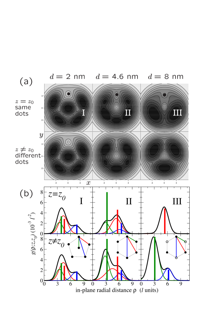
Figure 2: (a) Contour plot of the pair correlation function $P(\vect{\varrho},z;\vect{\varrho}_{0},z_{0})$ at various $d$-values. An electron is fixed at $(\vect{\varrho}_{0},z_{0})$ (black bullet) corresponding to a maximum of charge density. (b) Radial pair correlation function $g(\varrho;z,z_{0})$ vs $\varrho$. $g$ has been renormalized in such a way that $\int\!{\rm d}\vect{\varrho}\,g(\varrho;z,z_{0})=1$. Lengths are in units of $\ell=7.20$ nm [$\ell=(\hbar/m^{*}\Omega)^{1/2}$ characteristic in-plane radius]. Insets schematically show the spatial arrangement of electrons projected on the $xy$ plane.

To analyze the internal structure of the molecule, we compute the pair correlation function $P(\vect{\varrho},z;\vect{\varrho}_{0},z_{0})=\sum_{i\neq j}\left<\delta(\vect{\varrho}-\vect{\varrho_{i}})\delta(z-z_{i})\delta(\vect{\varrho_{0}}-\vect{\varrho_{j}})\delta(z_{0}-z_{j})\right>/N(N-1)$ (the average is on the ground state). Figure 2(a) shows a contour plot of $P(\vect{\varrho},z;\vect{\varrho}_{0},z_{0})$ at various values of $d$, one per column. An electron is fixed (black bullet) at the position $(\vect{\varrho}_{0},z_{0})$ in one dot, at the maximum of the charge density: the contour plots of the top (bottom) row, with $z=z_{0}=$ dot 1 ($z=$ dot 2, $z_{0}=$ dot 1) fixed, represent the conditional probability of measuring an electron in the $xy$ plane of dot 1 (2), given a first electron is fixed in dot 1. We find that the three phases we discussed above clearly show characteristic structural configurations (see also insets in Fig. 1): (I) At small $d$ (left column), the whole system is coherent. The electrons, delocalized over the dots, arrange at the vertices and the center of a regular pentagon. (II) At a critical value of $d=4.6$ nm (center) an abrupt transition takes place. In the new arrangement the electrons are at the vertices of a regular hexagon. Contrary to phase I, the peaks in the upper and lower dots have different heights. (III) When $d$ is further increased, the structure continuously evolves into two isolated dots (right), coupled only via Coulomb interaction. Three electrons in each dot sit at the vertices of two equilateral triangles rotated by 60 degrees.

Next we compare our system with its classical counterpart[13]. To this aim, we calculated the (circularly symmetric) radial pair correlation function $g(\varrho;z,z_{0})=\int\!{\rm d}\vect{\varrho_{0}}\,P(\vect{\varrho_{0}}+\vect{\varrho},z;\vect{\varrho_{0}},z_{0})$ vs $\varrho$, which gives the probability of finding an electron at a distance $\varrho$ from another one fixed on the same or opposite dot. For a classical system at zero temperature, $g$ consists of a set of $\delta$-function peaks. Figure 2(b) shows the calculated $g(\varrho;z,z_{0})$ for the same three configurations of 2(a), together with the histograms representing the equilibrium configuration of the corresponding classical system[13, 23]. When we fit $g$ to a set of gaussians, also shown in Fig. 2(b), we see that the agreement between “classical” and “quantum” cases is remarkable in phase III and, to a minor extent, in phase I, both from the point of view of absolute positions and relative intensities of the peaks. In contrast, in phase II the peaks of the quantum system resemble the classical ones just in position, while the intensities are definitely different; calculations show, moreover, that the relative intensities are strongly $d$-dependent. Classically, only phases I and III are ground-state configurations[13], while the hexagonal structure II is a metastable state[10]. Quantum fluctuations thus force a novel phase to appear.

We interpret the sequence I $\rightarrow$ II $\rightarrow$ III as a 2D $\rightarrow$ 3D $\rightarrow$ 2D transition. In phase III the motion is quasi-2D, with electrons occupying degenerate S and AS states to form a staggered configuration: the equilibrium structure corresponds to the classical one, with inter-dot tunneling absent. In phase II, instead, the motion acquires an effective $z$-component: as $d$ is decreased, electrons keep their electrostatic repulsion energy low at the expense of occupying AS states separated from S orbitals by an increasing energy gap. There is no classical analogue to this phase. When the gap becomes too large, the electrons abruptly arrange into I, all frozen in S orbitals. The motion now is that of a coherent quasi-2D QD, comparable to a classical single QD. To sum up, only in phase II electrons move in a truly 3D system: as shown in Fig. 2(a), the angular modulation of $P$ is much weaker than in I and III, suggesting that the crystallization regime has not been reached yet[2, 3].

There is another, more subtle, discrepancy between quantum and classical cases, due to the interplay of tunneling and particle indistinguishability. In phase I classical particles belong either to one dot or to the other, three each for $N=6$, and they can arrange in very asymmetric configurations in each dot, like in Fig. 1 of Ref. [13], provided that overall they form the centered pentagon which is favored by Coulomb interaction, the only energy scale in this case. In the quantum case, on the contrary, particles are equally delocalized on both dots. It simply makes no sense in this phase to assign electrons to a specific dot, since at small $d$ they can easily penetrate the inter-dot barrier. Therefore, tunneling changes the physics of the artificial molecule and actually drives phase I. Indeed, if we suppress tunneling (e.g., via a sufficiently high barrier), phase III is the only one present at any value of $d$, while phase I never shows up, contrary to the classical prediction[13].

We analyze the spectrum of neutral collective elementary excitations computing the dynamical form factor $S(L,\omega)=\sum_{n}|\langle n|\rho^{\dagger}_{L}|0\rangle|^{2}\,\delta\!\left(\omega-\omega_{n}+\omega_{0}\right)$, with $\left|n\right>$ ($\left|0\right>$) many-body $n$-th excited (ground) state with energy $\omega_{n}$ ($\omega_{0}$), $\omega$ excitation energy, $\rho^{\dagger}_{L}=\sum_{m}\sum_{g,g^{\prime}}c^{\dagger}_{L+m,g}c_{m,g^{\prime}}$ $L$-th angular component of density fluctuation. $S(L,\omega)$ assigns a weight to a charge density wave of angular momentum $L$ and energy $\omega$ in the excitation spectrum. Figure 3(a) shows $S(L,\omega)$ at low energies in the $d-\omega$ space; the intensity is proportional to the radius of circles. Only few branches are dominant in each phase, with a characteristic value of $|L|$: 5 in I, 6 or 3 in II and III, respectively. The occurrence of very few excitations with large values of $S(L,\omega)$[24] is remarkable: since the ground state is formed by a linear combination of thousands of Slater determinants with non-negligible weight, high values of the form factor are due to a constructive interference effect. Indeed, the geometry of the Wigner molecule selects the allowed –magic– values of $M$ and parity, and thus $L=M_{2}-M_{1}$ corresponding to the coupling between two magic states $M_{1}$, $M_{2}$. Consider, e.g., the wavefunction $\Psi$ of phase II with electrons at the vertices of a regular hexagon. A cyclic coordinate permutation is a $\pi/3$ rotation such that $\Psi\rightarrow\exp{(\pi{\rm i}M/3)}\Psi$. In this case $\Psi$ changes sign[25], and therefore $M=6p+3$ ($p$ integer) and odd parity. Our findings show that an excited magic state can be created adding $L$ quanta of angular momentum to the ground state via the density fluctuation operator $\rho^{\dagger}_{L}$. The allowed values of $L$ characterize different phases. The diamond shape of different $|L|$-branches in Fig. 3(a) originates from level crossing between magic states: $\omega\rightarrow 0$ at every $M$-transition in the ground state.

Finally, we compute the “electronic” part of Raman scattering cross section[26]. This is strictly related to $S(L,\omega)$, and is proportional to $\sum_{n}\left|M_{n0}\right|^{2}\delta\left(\omega-\omega_{n}+\omega_{0}\right)$, with $M_{n0}=\sum_{\alpha,\beta}\left<\alpha|{\rm e}^{{\rm i}\vect{q}\cdot\vect{r}}|\beta\right>\left<n|c^{\dagger}_{\alpha}c_{\beta}|0\right>$, and $\vect{q}$ wave vector transferred in the inelastic photon scattering[27]. The correlated excitation spectrum of single QDs has been already experimentally probed[28], in the regime $q\ell\approx 1$. Thus, having fixed a suitable value of $q$ in a backscattering geometry, in Figs 3(b) and (c) we plot the cross sections at different angles $\theta$ between $\vect{q}$ and the $xy$ plane ($\theta=0^{\circ}$ and $45^{\circ}$, respectively). The spectra resemble the form factor $S(L,\omega)$, but intensities are differently modulated. For in-plane scattering [Fig. 3(b), $\theta=0^{\circ}$], only the branches with $|L|=5$ characterizing phase I survive, while all other signals are suppressed. The background small dots appearing in Fig. 3(b-c) are smaller than 9 % of the maximum value. As $\theta$ increases [Fig. 3(c), $\theta=45^{\circ}$], the branches of phase I continuously loose intensity as those of II and III acquire weight, until the latter show a very strong signal at $\theta=45^{\circ}$, while the former are suppressed. In I, indeed, all electrons occupy S orbitals, hence the $z$-component $\int\!{\rm d}z\,\chi^{*}_{i}(z)\,{\rm e}^{{\rm i}q_{z}z}\chi_{j}(z)$ of matrix element $\left<\alpha|{\rm e}^{{\rm i}\vect{q}\cdot\vect{r}}|\beta\right>$ diminishes as long as $\theta$ (and $q_{z}$) increases; the opposite holds true for II and III, since S and AS orbitals can mix. This means that momentum can be transferred in the $z$-direction only in II and III, contrary to I, where the system is a unique quasi-2D dot. Signals with $|L|=6$ are almost invisible, but still phase II can be resolved from III in virtue of the characteristic energy and slope of visible branches. This comes from the way S and AS orbitals are differently filled in II and III, respectively, and hence from the different contribution of tunneling to the total energy. When $\theta$ is further increased, the selection rule $L=0$ becomes effective, and eventually at $\theta=90^{\circ}$ low-energy signals are suppressed.

To summarize, we have predicted a 2D-3D-2D transition of interacting electrons in a double QD, accompanied by the appearance of a novel liquid-like quantum phase, in addition to classical configurations. The $\theta$-dependent modulation of the Raman spectrum should allow to experimentally discriminate between different phases.

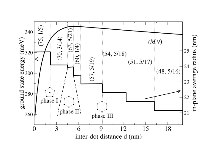
Figure 1: Ground-state energy (left axis) and in-plane average radius $\left<\varrho\right>$ (right axis) vs $d$ for $N=6$ at $B=25\,\mbox{T}$. For large $d$-values $M=36$ (not shown), twice than in a single QD with $N=3$. Insets show the electron arrangements in the different phases.

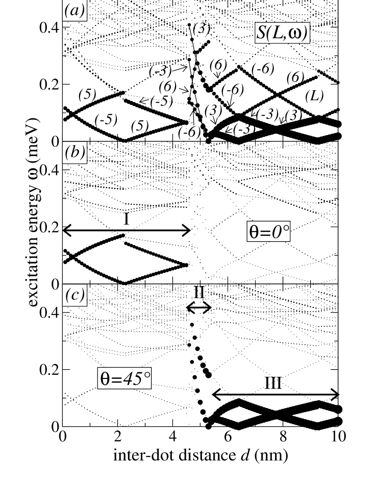
Figure 3: (a) Dynamical form factor $S(L,\omega)$ in the $d-\omega$ plane, for different angular momentum components $L$, indicated in parentheses. The radius of each point is proportional to its intensity. (b) Analogous plot for the Raman scattering cross section, at an angle $\theta=0^{\circ}$ between the $xy$ plane and the transferred momentum $\vect{q}$ ($q=2\cdot 10^{6}$ cm^-1). (c) Same as (b), with $\theta=45^{\circ}$.

- [1] \NameWigner E. \REVIEWPhys. Rev.4619341002; \NameIshiara A. \REVIEWSolid State Phys.421989271; \NameCôté R. \BookMicroscopic Theory of Semiconductors \EditorS. W. Koch \PublWorld Scientific, London \Year1995 \Page315.
- [2] \NameCeperley D. M. Alder B. J. \REVIEWPhys. Rev. Lett.451980566; \NameTanatar B. Ceperley D. M. \REVIEWPhys. Rev. B3919895005.
- [3] \NameLam P. K. Girvin S. M. \REVIEWPhys. Rev. B301984473.
- [4] \NameGrimes C. C. Adams G. \REVIEWPhys. Rev. Lett.421979795.
- [5] \NameManoharan H. C., Suen Y. W., Santos M. B. Shayegan M. \REVIEWPhys. Rev. Lett.7719961813.
- [6] \NameJacak L., Hawrylak P., Wójs A. \BookQuantum Dots \PublSpringer, Berlin \Year1998.
- [7] For a review see \NameMaksym P. A., Imamura H., Mallon G. P. Aoki H. \REVIEWJ. of Phys.: Cond. Mat.122000R299.
- [8] \NameBryant G. W. \REVIEWPhys. Rev. Lett.5919871140; \NameYannouleas C. Landman U. \SAME8219995325; \SAME8520002220(E); \NameEgger R., Häusler W., Mak C. H. Grabert H. \SAME8219993320; \SAME831999462(E); \NameReimann S. M., Koskinen M. Manninen M. \REVIEWPhys. Rev. B6220008108; \NameMüller H.-M. Koonin S. E. \SAME54199614532.
- [9] \NameFilinov A. V., Bonitz M. Lozovik Yu. E. \REVIEWPhys. Rev. Lett.8620013851.
- [10] \NameBolton F. Rössler U. \REVIEWSuperlatt. and Microstruct.131993139; \NameBedanov V. M. Peeters F. M. \REVIEWPhys. Rev. B4919942667.
- [11] \NameKouwenhoven L. \REVIEWScience26819951440.
- [12] \NameRontani M., Troiani F., Hohenester U. Molinari E. \REVIEWSolid State Commun.1192001309; \NameRontani M., Rossi F., Manghi F. Molinari E. \SAME1121999151.
- [13] \NamePartoens B., Schweigert V. A. Peeters F. M. \REVIEWPhys. Rev. Lett.7919973990.
- [14] \NamePalacios J. J. Hawrylak P. \REVIEWPhys. Rev. B5119951769.
- [15] \NameImamura H., Maksym P. A. Aoki H. \REVIEWPhys. Rev. B53199612613; \SAME5919995817. Authors identify phases I and III for .
- [16] \NamePartoens B., Matulis A. Peeters F. M. \REVIEWPhys. Rev. B5919991617.
- [17] \NameFilinov A. V., Bonitz M. Lozovik Yu. E. \REVIEWContrib. Plasma Phys.4120011/2.
- [18] At larger spin plays an important role; for example, in the regime close to total filling factor two, it may give rise to a non trivial phase diagram [\NameMartín-Moreno L., Brey L. Tejedor C. \REVIEWPhys. Rev. B622000R10633].
- [19] We assumed T, and , , , , , , as typical values of realistic devices [Cf. \NamePi M., Emperador A., Barranco M., Garcias F., Muraki K., Tarucha S. Austing D. G. \REVIEWPhys. Rev. Lett.87200166801].
- [20] \NameMaksym P. A. Chakraborty T. \REVIEWPhys. Rev. Lett.651990108.
- [21] \NameLaughlin R. B. \REVIEWPhys. Rev. B2719833383.
- [22] \NameŚwierkowski L., Neilson D. Szymański J. \REVIEWPhys. Rev. Lett.671991240; \NameGoldoni G. Peeters F. M. \REVIEWEurophys. Lett.371997293.
- [23] For the classical histograms, we used data of a single QD [\NameDate G., Murthy M. V. N. Vathsan R. \REVIEWJ. of Phys.: Cond. Mat.1019985876]: II differs from III in the way electrons are placed on a particular dot. We normalized -functions so that the two highest classical and quantum peaks in III have the same height.
- [24] The value of dots not labeled by in Fig. 3(a) is smaller than 16 % of the maximum value.
- [25] \NameRuan W. Y., Liu Y. Y., Bao C. G. Zhang Z. Q. \REVIEWPhys. Rev. B5119957942.
- [26] \NameHawrylak P. \REVIEWSolid State Commun.931995915.
- [27] \NameBlum F. A. \REVIEWPhys. Rev. B119701125.
- [28] \NameLockwood D. J., Hawrylak P., Wang P. D., Sotomayor Torres C. M., Pinczuk A. Dennis B. S. \REVIEWPhys. Rev. Lett.771996354; \NameSchüller C., Keller K., Biese G., Ulrichs E., Rolf L., Steinebach C., Heitmann D. Eberl K. \SAME8019982673.