Vortex Rings and Lieb Modes in a Cylindrical Bose-Einstein Condensate

Abstract

We present a calculation of a solitary wave propagating along a cylindrical Bose-Einstein trap, which is found to be a hybrid of a one-dimensional (1D) soliton and a three-dimensional (3D) vortex ring. The calculated energy-momentum dispersion exhibits characteristics similar to those of a mode proposed sometime ago by Lieb within a 1D model, as well as some rotonlike features.

Approximately forty years ago, Lieb and Liniger lieb1 employed the Bethe Ansatz to obtain an exact diagonalization of the model Hamiltonian that describes a one-dimensional (1D) Bose gas interacting via a repulsive $\delta$-function potential. Based on this solution Lieb lieb2 proposed an intriguing dual interpretation of the spectrum of elementary excitations, either in terms of the familiar Bogoliubov mode, or in terms of a certain kind of a particle-hole excitation which will hereafter be referred to as the Lieb mode. The energy-momentum dispersions of the Bogoliubov and the Lieb modes coincide at low momenta, where they both display the linear dependence characteristic of sound-wave propagation in an interacting Bose-Einstein Condensate (BEC), but the Lieb dispersion is significantly different at finite momenta where it exhibits a surprising $2\pi$ periodicity. Yet this new mode remained somewhat of a theoretical curiosity because of the absence of a physical realization of a strictly 1D Bose gas.

In a curious turn of events, the above subject re-emerged in connection with the solitary waves calculated analytically within a 1D classical Gross-Pitaevskii (GP) model tsuzuki ; zakharov , which were later shown to provide an approximate but fairly accurate description of the quantum Lieb mode for practically all coupling strengths kulish ; ishikawa . More importantly, the same solitary waves motivated experimental observation of similar coherent structures in BEC of alkali-metal atoms through phase imprinting or phase engineering burger ; denschlag . Therefore, an opportunity presents itself for experimental realization of the Lieb mode.

It is clear that a theoretical investigation based on effective 1D models often used to describe cylindrical traps will lead to the prediction of a Lieb mode, by arguments similar to those employed in the original 1D classical model kulish ; ishikawa . However, one should also question the stability of the corresponding solitons within the proper 3D environment of a realistic trap muryshev ; feder . For example, dark solitons created within a spherical trap were observed to decay into vortex rings anderson . This observation was also supported by a numerical calculation in which an initial dark-soliton configuration is let to evolve in time according to the GP equation.

Therefore, although the production of solitary waves through phase imprinting clearly suggests some distinct 1D characteristics, it should be expected that a proper understanding of such waves must also account for 3D effects that are inevitably present in a realistic BEC. One could envisage a picture in which the actual solitary wave is a hybrid of a 1D soliton and a 3D vortex ring. It is the aim of the present paper to make the above claim precise by calculating solitons propagating along a cylindrical trap without making a priori assumptions about their effective dimensionality. Our approach was motivated by the calculation of vortex rings in a homogeneous BEC due to Jones and Roberts jones1 and a similar calculation of semitopological solitons in planar ferromagnets semi .

Explicit results will be presented for a set of parameters that roughly correspond to the experiment of Ref. burger . Thus we consider a cigar-shaped trap filled with ⁸⁷Rb atoms, with a transverse confinement frequency $\omega_{\bot}\!=\!2\pi\!\times\!425$ Hz and a corresponding oscillator length $a_{\bot}\!=\!\sqrt{\hbar/m\omega_{\bot}}\!\approx\!0.5\mu m$. The coupling constant is written as $U_{o}\!=\!4\pi\hbar^{2}a/m$ where $a\!\approx\!50\,\hbox{\AA}$ is the scattering length. We make the approximation of an infinitely-long cylindrical trap with average linear density $\nu\!=\!0.2\,\hbox{atoms}/\hbox{\AA}$ and introduce the dimensionless combinations of parameters $\gamma\!=\!\nu a\!=\!10$ and $\gamma_{\bot}\!=\!\nu a_{\bot}\!=\!10^{3}$. Finally, rationalized units are defined through the rescalings $t\!\to\!t/\omega_{\bot},\;\;{{\hbox{\bf r}}}\!\to\!a_{\bot}{{\hbox{\bf r}}},\;\;\hbox{and}\;\;\Psi\!\to\!\sqrt{\nu}\,\Psi/a_{\bot}\,$.

The energy functional extended to include a chemical potential is then given by

$$W=\frac{1}{2}\int{\left[\bm{\nabla}\Psi^{*}\bm{\nabla}\Psi+\rho^{2}\,\Psi^{*}\Psi+g(\Psi^{*}\Psi)^{2}-2\mu\,\Psi^{*}\Psi\right]\,dV},$$ (1)

where $g\!=\!4\pi\gamma$ and $\rho^{2}\!=\!x^{2}+y^{2}$, and yields energy in units of $\gamma_{\bot}\hbar\omega_{\bot}$ while the chemical potential $\mu$ is still measured in units of $\hbar\omega_{\bot}$. Similarly, the conserved linear momentum along the $z$ axis given by the usual definition

$${\cal P}=\frac{1}{2i}\,\int{\left(\Psi^{*}\frac{\partial\Psi}{\partial z}-\frac{\partial\Psi^{*}}{\partial z}\Psi\right)\;dV}=\int{n\frac{\partial\phi}{\partial z}\;dV},$$ (2)

is measured in units of $\hbar\nu\!=\!\gamma_{\bot}(\hbar/a_{\bot})$. In the second step of Eq. (2) we employed the usual hydrodynamic variables defined from $\Psi\!=\!\sqrt{n}\,e^{i\phi}$.

Figure 1: Radial dependence of the solitary wave function at $v\!=\!c/2$ for various positive values of $\xi$ in steps of $\delta\xi\!=\!0.1$. The result for negative $\xi$ is obtained through the symmetry relations $\hbox{Re}\,\Psi(\rho,\xi)\!=\!\hbox{Re}\,\Psi(\rho,-\xi)$ and $\hbox{Im}\,\Psi(\rho,\xi)\!=\!-\hbox{Im}\,\Psi(\rho,-\xi)$. Distances are measured in units of $a_{\bot}$.

An important first step in out calculation was to obtain accurate information about the ground state and the corresponding linear (Bogoliubov) modes. The ground-state wave function $\Psi\!=\!\Psi_{0}(\rho)$ was calculated as a stationary point of the energy functional (1) by a variant of a relaxation algorithm dalfovo and is normalized according to $\int_{0}^{\infty}{2\pi\rho\,d\rho\;|\Psi_{0}|^{2}}\!=\!1$ to conform with our choice of rationalized units. The chemical potential was found to be $\mu\!=\!6.4324$ for $\gamma\!=\!10$. We have also recalculated the lowest branch of the Bogoliubov spectrum from which we extracted the speed of sound $c\!=\!1.77$ in units of $a_{\bot}\omega_{\bot}$. This numerical estimate at $\gamma\!=\!10$ is consistent to within 1% with the Thomas-Fermi approximation $c\!=\!\gamma^{1/4}$ which was previously derived in a number of papers zaremba ; kavoulakis ; stringari and was employed for the analysis of experimental data andrews .

Thus we turn to the calculation of axially-symmetric solitary waves described by a wave function of the form $\Psi\!=\!\Psi(\rho,\xi)$ where $\xi\!=\!z-vt$ and $v$ is the constant velocity along the $z$ axis. Such a wave function satisfies the stationary differential equation

$$-iv\,\frac{\partial\Psi}{\partial\xi} = -\frac{1}{2}\Delta\Psi+\frac{1}{2}\rho^{2}\Psi+g(\Psi^{*}\Psi)\Psi-\mu\Psi\,,$$ (3)

$$\Delta = \frac{\partial^{2}}{\partial\rho^{2}}+\frac{1}{\rho}\frac{\partial}{\partial\rho}+\frac{\partial^{2}}{\partial\xi^{2}}\,,$$

which is supplemented by the boundary conditions that $\Psi$ vanish for $\rho\!\to\!\infty$, and $|\Psi|\!\to\!|\Psi_{0}(\rho)|$ for $\xi\!\to\!\pm\infty$. The phase of the wave function is not fixed a priori at spatial infinity, except for a mild restriction implied by the Neumann boundary condition $\partial\Psi/\partial\xi\!=\!0$ imposed at $\xi\to\pm\infty$ mainly for numerical purposes. Finally, a solution of Eq. (3) must satisfy the virial relation

$$v\,{\cal P}=\int{\left[\frac{1}{2}\frac{\partial\Psi^{*}}{\partial\xi}\frac{\partial\Psi}{\partial\xi}+\rho^{2}\,\Psi^{*}\Psi+\frac{g}{2}(\Psi^{*}\Psi)^{2}-\mu\Psi^{*}\Psi\right]dV}\,,$$ (4)

obtained by a standard scaling argument.

Figure 2: Radial dependence of the local particle density $n\!=\!|\Psi|^{2}$ for the four special cases discussed in the text. Conventions are the same as in Fig. 1.

Solutions of Eq. (3) were obtained by a sophisticated Newton-Raphson iterative algorithm jones1 ; semi which will not be described here in any detail. For values of the velocity $v$ near the speed of sound $c$, the calculated solitary wave is a rarefaction pulse that may be thought of as a mild soundlike disturbance of the ground state. The dominant features of the solitary wave are pronounced as the velocity is decreased to lower values and become reasonably apparent at $v\!=\!c/2$, as shown in Fig. 1 which provides a complete illustration of the wave function through its real and imaginary parts. A partial but more transparent illustration is given in frame I of Fig. 2 where we depict the radial dependence of the local particle density $n\!=\!|\Psi|^{2}$ for various values of $\xi$. It is clear that the density near the center of the soliton ($\xi\!=\!0$) vanishes on a ring with a relatively large radius $R\!\simeq\!2.8$, thus a vortex ring is beginning to emerge. The features of the vortex ring become completely apparent, and its radius is tightened, as we proceed to yet smaller values of the velocity. A notable special case is the static ($v\!=\!0$) vortex ring with radius $R\!\simeq\!1.8$ illustrated in frame II of Fig. 2, which is far from being a completely dark (black) solitary wave.

One would think that pushing the velocity $v$ to negative values would retrace the calculated sequence of solitary waves backwards. In fact, our algorithm continues to converge to vortex rings of smaller radii until a critical velocity $v\!=\!-v_{0}\!\simeq\!-0.475\,c$ is encountered where the vortex ring achieves its minimum radius $R_{\rm min}\!\simeq\!0.8$ and ceases to exist for smaller values of $v$. The terminal state at $v\!=\!-v_{0}$ is illustrated in frame III of Fig. 2. We have thus described a sequence of solitary waves with velocities in the range $-v_{0}\!<\!v\!<\!c$, which does not contain a black soliton. An equivalent sequence is obtained in the range $-c\!<\!v\!<\!v_{0}$ simply by reversing the relative sign between the real and imaginary part of the wave function, as is evident from Eq. (3).

It is now important to calculate the energy-momentum dispersion. The excitation energy is defined as $E\!=\!W-W_{0}$ where both $W$ and $W_{0}$ are calculated from Eq. (1) applied for the solitary wave $\Psi(\rho,\xi)$ and the ground state $\Psi_{0}(\rho)$, respectively. The presence of the chemical potential in Eq. (1) provides the compensation that is necessary in order to compare energies of states with the same number of particles. Similarly, the relevant “physical” momentum is not the linear momentum ${\cal P}$ of Eq. (2) but the “impulse” $Q$ defined in a manner analogous to the case of a homogeneous gas ishikawa ; jones1 :

$$Q = \int{(n-n_{0})\frac{\partial\phi}{\partial z}\,dV}={\cal P}-\delta\phi$$ (5)

$$\delta\phi \equiv \int_{0}^{\infty}{2\pi\rho\,d\rho\;n_{0}(\rho)[\phi(\rho,z\!=\!\infty)-\phi(\rho,z\!=\!-\infty)]}\,,$$

where $n_{0}\!=\!|\Psi_{0}(\rho)|^{2}$ is the ground-state particle density and $\delta\phi$ is the weighted average of the phase difference between the two ends of the trap. Here we simply postulate the validity of definition (5) and note that the corresponding group-velocity relation $v\!=\!dE/dQ$ was satisfied to an excellent accuracy in our numerical calculation. On the other hand, the virial relation (4) was verified using the standard linear momentum ${\cal P}$ of Eq. (2), as expected.

Figure 3: Energy $E$ in units of $\gamma_{\bot}(\hbar\omega_{\bot})$ versus impulse $Q$ in units of $\gamma_{\bot}(\hbar/a_{\bot})$. The solid line corresponds to the main sequence of solitary waves discussed in the text, and the dashed line to the auxiliary sequence that contains a black soliton (point IV).

The calculated dispersion $E\!=\!E(Q)$ is depicted in Fig. 3 by a solid line along which we place the symbols I, II and III that correspond to the special cases of the solitary wave discussed above. At low $Q$ the dispersion is linear, $E\!=\!c\,|Q|$, a feature that it shares with the Bogoliubov dispersion. However, the energy now reaches a maximum at point II where $v\!=\!0$ and $Q$ is slightly greater that $\pi$. Interestingly, the group velocity becomes negative in the region (II,III) or, equivalently, the impulse is opposite to the group velocity. This rotonlike behavior could develop into a full-scale roton if the terminal point III actually turns out to be an inflection point beyond which the group velocity may begin to rise again. We have not been able to somehow continue our sequence of solitary waves beyond point III, nor have we ruled out such a possibility. In any case, the picture just described, together with the fact that the calculated radius of the vortex ring is monotonically decreasing along the sequence (I,II,III) comes close to the Onsager-Feynman view of a roton as the ghost of a vanished vortex ring donnelly .

The branch of the dispersion shown by a solid line in Fig. 3 was calculated on the basis of the sequence of solitary waves with velocities in the range $-v_{0}\!<\!v\!<\!c$. The branch for $-c\!<\!v\!<\!v_{0}$ may be thought to correspond to negative $Q$, as usual. However, there is an implicit $2\pi$ periodicity because of the appearance of the angle $\phi$ in the definition of the impulse in Eq. (5). Therefore, a more natural representation of the spectrum seems to be obtained by restricting $Q$ to the “first Brillouin zone” and thus completing Fig. 3 by its mirror image around $Q\!=\!\pi$.

We have also carried out a detailed numerical calculation of the Bogoliubov dispersion for comparison. But the main point can be made here by assuming the model dispersion $\omega=|q|(c^{2}+q^{2}/4)^{1/2}$ where the frequency $\omega$ is measured in units of $\omega_{\bot}$ and the wave number $q$ in units of $1/a_{\bot}$. Translated into the units employed in Fig. 3, the model Bogoliubov dispersion reads $E=|Q|(c^{2}+\gamma_{\bot}^{2}Q^{2}/4)^{1/2}$ where a huge factor $\gamma_{\bot}^{2}\!\approx\!10^{6}$ makes its appearance. Therefore, although the Bogoliubov and Lieb dispersions coincide at low $Q$, they diverge quickly at the scale of Fig. 3, a notable difference from the homogeneous 1D model lieb2 ; ishikawa . In other words, the two modes operate at rather different energy and momentum scales in a cylindrical trap.

The last question we address is whether or not there exists an independent sequence of solitary waves that reduces to a black soliton at $v\!=\!0$. We used a model black-soliton configuration as input in our iterative algorithm which converged to the true static soliton illustrated in frame IV of Fig. 2 that is indeed a black soliton. We then incremented the velocity to either positive or negative values with symmetrical results. For definiteness, we follow the solution to negative $v$ and find that it exists only until one encounters the same critical velocity $-v_{0}$ discussed earlier in the text. The corresponding terminal state is precisely the same with the one reached through our original sequence of solitary waves and illustrated in frame III of Fig. 2. For intermediate values of $v$ the solution is again a vortex ring with constant radius at $R\!=\!R_{\rm min}\!\approx\!0.8$. Accordingly, the calculated energy-momentum dispersion shown by a dashed line in Fig. 3 joins the original sequence through a cusp at the terminal point III, a situation that is reminiscent of the calculation of Jones and Roberts jones1 . The same authors together with Putterman later argued jones2 that the solitary waves that correspond to the upper branch are actually unstable, a conclusion that might be valid in the present case as well.

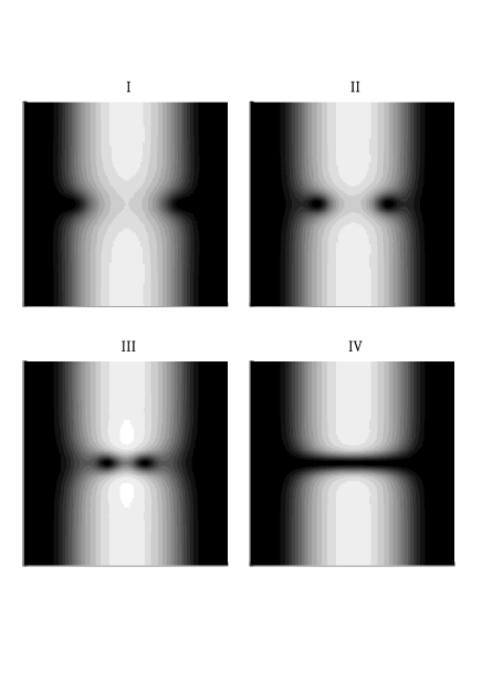
Figure 4: Contour levels of the local particle density $n$ in a plane that contains the $z$ axis and cuts across the cylindrical trap. The complete 3D picture may be envisaged by simple revolution around the $z$ axis. Regions with high particle density are bright while regions with zero density are black. The four special cases considered are the same as in Fig. 2.

A summary view of our results is given in Fig. 4. We have thus constructed a family of solitary waves which exhibit some quasi-1D features, such as the appearance of a nontrivial phase difference $\delta\phi$ that is important for phase engineering burger ; denschlag , but are otherwise bonafide 3D vortex rings.

We are grateful to G.M. Kavoulakis for numerous discussions that guided us through the extensive recent literature on BEC. S.K. acknowledges financial support from the Gratuiertenkolleg “Non-equilibrium phenomena and phase transitions in complex systems” and thanks the University of Crete and the Research Center of Crete for hospitality.

References

- (1) E.H. Lieb and W. Liniger, Phys. Rev. 130, 1605 (1963).
- (2) E.H. Lieb, Phys. Rev. 130, 1616 (1963).
- (3) T. Tsuzuki, J. Low Temp. Phys. 4, 441 (1971).
- (4) V.E. Zakharov and A.B. Sabat, Sov. Phys. JETP 37, 823 (1973).
- (5) P.P. Kulish, S.V. Manakov, and L.D. Faddeev, Theor. Math. Phys. 28, 615 (1976).
- (6) M. Ishikawa and H. Takayama, J. Phys. Soc. Japan 49, 1242 (1980).
- (7) S. Burger, K. Bongs, S. Dettmer, W. Ertmer, K. Sengstock, A. Sanpera, G.V. Shlyapnikov, and M. Lewenstein, Phys. Rev. Lett. 83, 5198 (1999).
- (8) J. Denschlag, J. E. Simsarian, D. L. Feder, Charles W. Clark, L.A. Collins, J. Gubizolles, L. Deng, E.W. Hagley, K. Helmerson, W.P. Reinhardt, S.L. Rolston, B.I. Schneider, and W.D. Phillips, Science 287, 97 (2000).
- (9) A.E. Muryshev, H.B. van Linden van den Heuvell, and G.V. Shlyapnikov, Phys. Rev. A 60, R2665 (1999).
- (10) D.L. Feder, M.S. Pindzola, L.A. Collins, B.I. Schneider, and C.W. Clark, Phys. Rev. A 62, 053606 (2000).
- (11) B.P. Anderson, P.C. Haljan, C.A. Regal, D.L. Feder, L.A. Collins, C.W. Clark, and E.A. Cornell, Phys. Rev. Lett. 86, 2926 (2001).
- (12) C.A. Jones and P.H. Roberts, J. Phys. A: Math. Gen. 15, 2599 (1982).
- (13) N. Papanicolaou and P.N. Spathis, Nonlinearity 12, 285 (1999).
- (14) F. Dalfovo and S. Stringari, Phys. Rev. A 53, 2477 (1996).
- (15) E. Zaremba, Phys. Rev. A 57, 518 (1998).
- (16) G.M. Kavoulakis and C.J. Pethick, Phys. Rev. A 58, 1563 (1998).
- (17) S. Stringari, Phys. Rev. A 58, 2385 (1998).
- (18) M.R. Andrews, D.M. Kurn, H.-J. Miesner, D.S. Durfee, C.G. Townsend, S. Inouye, and W. Ketterle, Phys. Rev. Lett. 79, 553 (1997); ibid 80, 2967 (1998).
- (19) R.J. Donnelly, Quantized Vortices in Helium II, (Cambridge University Press, 1991).
- (20) C.A. Jones, S.J. Putterman, and P.H. Roberts, J. Phys. A: Math. Gen. 19, 2991 (1986).