Statistical properties of charged interfaces

Abstract

We consider the equilibrium statistical properties of interfaces submitted to competing interactions; a long-range repulsive Coulomb interaction inherent to the charged interface and a short-range, anisotropic, attractive one due to either elasticity or confinement. We focus on one-dimensional interfaces such as strings. Model systems considered for applications are mainly aggregates of solitons in polyacetylene and other charge density wave systems, domain lines in uniaxial ferroelectrics and the stripe phase of oxides. At zero temperature, we find a shape instability which lead, via phase transitions, to tilted phases. Depending on the regime, elastic or confinement, the order of the zero-temperature transition changes. Thermal fluctuations lead to a pure Coulomb roughening of the string, in addition to the usual one, and to the presence of angular kinks. We suggest that such instabilities might explain the tilting of stripes in cuprate oxides. The $3D$ problem of the charged wall is also analyzed. The latter experiences instabilities towards various tilted phases separated by a tricritical point in the elastic regime. In the confinement regime, the increase of dimensionality favors either the melting of the wall into a Wigner crystal of its constituent charges or a strongly inclined wall which might have been observed in nickelate oxides.

I Introduction

Various types of systems display peculiar properties due to competing long-range forces. In this paper we focus on the statistical properties of charged interfaces, in Ising-like systems, such as aggregates of charged topological defects in charge-density wave systems SBNK ; Yu Lu and among them polyacetylene Heeger , charged domain-lines in uniaxial ferroelectrics Monceau or stripes in oxides Tranq ; Zaanen . Instabilities, such as the observed inclination of stripes in cuprates incli and manganese Dai , might be related to the presence of the long range Coulomb interactions and its competition with an attractive force. Uniaxial ferroelectrics and density waves are also model systems where such instabilities could take place. The present study deals with one or two-dimensional charged interfaces, i.e. strings or walls. The former is realized in oxides, monolayers of doped conducting polymers or other charge-density waves and junctions in field effect experiments battlogg for equivalent materials. The latter might be present, due to a dimensional crossover which induces a $3D$ ordering, in the systems cited above.

The above interests emerged from a model-independent theory concerning the statistical and thermodynamic properties of uncharged and charged solitons which has been studied, respectively, in Refs. bohr, and teber, . The system considered is two-fold degenerate and, when topologically doped, the solitons form a one-component plasma in either $2$ or $3D$ space. The competition between the long-range $3D$ Coulomb interaction of the particles and the confinement force between them has led to a very rich phase diagram. Particularly interesting was the regime where the temperature is much less than the confinement energy scale, so that the solitons are actually bound into pairs, and the repulsive Coulomb interaction is weak enough to preserve these bisolitons as the elementary particles. In this regime, aggregated phases of bisolitons were shown to exist. The study of such aggregates in the continuum limit is equivalent to the study of charged interfaces.

The statistical properties of charged fluctuating manifolds have been considered before mehran . In this study, the authors have been considering a generalization of the theory of polyelectrolytes, cf. Ref. orland, , and have been focusing on the properties emerging from scale invariance and renormalization. Even though some of our results will converge with the previous study, which seems to be quite natural, our aim will be different. We consider interfaces directed along an anisotropy axis of the system which are either in an elastic or confinement regime; the latter is relevant to quasi-one dimensional systems in relation with the statistical properties of solitons mentioned above. In both regimes the Coulomb interaction favors the disintegration of the interface. In contrast with the instability towards a modulation which has been suggested in Ref. teber, this competition, as we will show, leads to zero-temperature shape instabilities with respect to a tilting of the interface. We will focus mainly on the properties related to this discrete symmetry breaking. This will able us to better understand the structure of the solitonic lattice in the presence of the long range repulsive interaction. In this respect, and as explained in teber , even though this problem seems to be quite old, the detailed impact of the Coulomb interaction has not been reported before. Moreover, the charged solitonic lattice is commonly observed nowadays as stripes in various oxides. Experimentally the observation that upon doping the system, at low temperatures, a transition from a collinear, i.e. vertical, to a diagonal stripe phase takes place incli is strikingly similar to our actual results.

The paper is organized as follows. We will mainly concentrate on the statistical properties of a charged string. In section II we present the models of the confined and elastic charged strings. In section III we derive the statistical properties of the string with the help of a saddle-point calculation. We present the zero-temperature results dealing with the instabilities of the string. In section IV the effects of thermal fluctuations are considered. In section V the previous results are confirmed with the help of a numerical approach. In section VI the present study is applied to the $2D$ and $3D$ solitonic lattices, as well as stripes and uniaxial ferroelectrics.

II Elastic and confinement regimes for the charged string

The problem of the charged string teber has emerged from the study of the statistical properties of topological defects, i.e. solitons, common to charge density wave (CDW) systems. These general arguments are reproduced in the following as they give a full meaning to the physical origins of the present theory, cf. SBNK for a review on the physics of topological defects in CDW systems. It should however be clear that this study is also relevant to other systems with discrete symmetry breaking as has been mentioned already in the Introduction.

For the moment we consider a one-dimensional system, i.e. a single chain, in a CDW state. The latter is described by a lattice order parameter which is complex in general

$$\Delta(x)=|\Delta(x)|\exp(i\varphi(x))$$

where $x$ runs along the chain, $|\Delta(x)|$ is related to the CDW gap and $\varphi(x)$ fixes the position of the CDW with respect to a host lattice. In weakly commensurate CDW the low energy excitations are excitations of the phase. This leads, cf. schultz , to a sine-Gordon type Hamiltonian

$$H=\int dx\left(\frac{\hbar v_{F}}{2\pi}\left(\frac{\partial\varphi}{\partial x}\right)^{2}-W\cos\left(M\varphi\right)\right)$$ (1)

where the first term gives the elastic energy of the CDW and the second term reflects the pinning of the CDW superstructure by the host lattice; $M$ is the degeneracy of the ground-state.

The non-trivial solutions of the equation of motion associated with (1) are the solitons, i.e. the $\varphi-$particles rice , which may be viewed as compressions or dilatations of the CDW. As we are in the realm of electronic crystals the solitons might therefore carry a charge which is fractional, i.e. $q=2/M$, in the general case. For a double-degenerate ground state, $M=2$, they are given by

$$\varphi(x)=2\arctan\left(\exp(2x/\xi)\right)$$ (2)

where the length $\xi\sim\sqrt{\hbar v_{F}/W}$ corresponds to the width of this nucleus domain wall connecting the two ground states $\varphi(\pm\infty)=\pm 1$.

The situation is slightly different for the two-fold degenerate trans-polyacetylene because in this case the band is half-filled and the system is commensurate. In particular equation (1) does not describe this case. However the previous arguments remain qualitatively the same. The defect is an amplitude or $\pi-$soliton; it carries an integer charge and is described by

$$\Delta(x)=\Delta_{0}\tanh(x/\xi)$$ (3)

where $\Delta_{0}$ is a constant deformation of the chains. Again this excitation connects the two ground states of the system $\Delta(\pm\infty)=\pm\Delta_{0}$.

For a quasi-one-dimensional system, which we consider here, neighboring chains must have the same phase modulo $2\pi$. This leads to the following general two-particle interaction

$$E(\delta x)=-V\int dz\Delta_{\alpha}(\delta x-z)\Delta_{\beta}(z)$$ (4)

between neighboring chains $\alpha$ and $\beta$, with coupling constant $V$, and solitons distant by $\delta x$. In the coarse-grained regime, $\delta x\gg\xi$, (4) grows linearly, $E\approx V\delta x$, a signature of the confinement of the defects. This can be shown explicitly with the help of (3) and (4). Dealing with a string, e.g. a domain line of solitons, this confinement energy is equivalently reproduced by the Solid on Solid (SOS) model. The related Hamiltonian reads

$$H_{conf}=\frac{J_{\perp}}{a_{y}}\sum^{L-1}_{y=0}|x_{y+1}-x_{y}|$$ (5)

where we have taken $J_{\perp}=Va_{y}$ as the inter-chain energy scale, $y$ runs along the vertical direction and $x_{y}$ is an integer variable giving the deviation of the string with respect to the $y$ axis.

The opposite case, corresponding to small deviations $\delta x\ll\xi$, is more general for the energy then increases quadratically $E\approx V\delta x^{2}$. This is equivalent to the elastic model which is extensively used in interface physics. The related Hamiltonian reads

$$H_{elast}=J_{\perp}\int\frac{dy}{a_{y}}\left(\frac{dx}{dy}\right)^{2}.$$ (6)

These two interface models are well known forgacs . To compactify notations we shall define

$$H_{0p}=J_{\perp}\int\frac{dy}{a^{p}_{y}}|\frac{dx}{dy}|^{p}$$ (7)

where $p=1,2$ leading respectively to the confinement and elastic regimes and where the continuum limit has been taken in both cases. We thus see that a crossover (corresponding to fractional $1<p<2$) from the elastic to the confinement regime takes place as the distance between solitons increases, i.e. as the tilt angle of the string increases. This is manifested by the fact that $\delta x=(dx/dy)a_{y}=\zeta a_{y}$ where $\zeta$ is related to the tilt angle of the string and $a_{y}$ is the inter-chain distance. For $\zeta\ll\xi/a_{y}$ the string is elastic whereas for $\zeta\gg\xi/a_{y}$ the confined string is relevant. The crossover between the two regimes takes place at

$$\zeta_{0}=\xi/a_{y}.$$ (8)

The introduction of the $3D$ long-range Coulomb interaction yields

$$H_{c}=\frac{(ze)^{2}}{2\epsilon}\int\int dydy^{\prime}\left(\frac{1}{\sqrt{(y-y^{\prime})^{2}+(x(y)-x(y^{\prime}))^{2}}}-\frac{1}{\sqrt{(y-y^{\prime})^{2}}}\right)$$ (9)

where $z\leq 1$ so that the elementary constituent of the string might carry a fractional charge $ze$ ($z=1$ for polyacetylene), $\epsilon$ is the dielectric constant of the isotropic, neutral media in which the plane is embedded and the contribution of the vertical string has been subtracted.

The thermodynamics of the charged interface is governed by $H_{p}=H_{0p}+H_{c}$ or explicitly

$$H_{p}=J_{\perp}\int\frac{dy}{a^{p}_{y}}|\frac{dx}{dy}|^{p}+\frac{(ze)^{2}}{2\epsilon}\int\int dydy^{\prime}\left(\frac{1}{\sqrt{(y-y^{\prime})^{2}+(x(y)-x(y^{\prime}))^{2}}}-\frac{1}{|y-y^{\prime}|}\right).$$ (10)

III The charged string at zero temperature

III.1 The saddle point approximation

We consider a configuration

$$x(y)=x^{(0)}(y)+\delta x(y)$$ (11)

were $x(y)$ has been expanded in the vicinity of the saddle point distribution $x^{(0)}(y)$ with deviations $\delta x(y)$. Free boundary conditions are taken. The expanded Hamiltonian reads, in the harmonic approximation

$$H_{p}=H_{p}^{(0)}+\frac{1}{2}\int\int dydy^{\prime}\delta x(y)\delta^{(2)}H/\delta x(y)\delta x(y^{\prime})|_{\delta x=0}\delta x(y^{\prime})+...$$ (12)

where $H_{p}$ is given by (10) and $H_{p}^{(0)}\equiv H_{p}\{\delta x^{(0)}(y)\}$. The saddle point distribution is given by $\delta H_{p}/\delta x(y)=0$ that is

$$J_{\perp}p\left(\Delta x^{(0)}(y)\right)^{p-1}=\frac{(ze)^{2}}{2\epsilon}\int^{+\infty}_{-\infty}dy^{\prime}\frac{x^{(0)}(y^{\prime})-x^{(0)}(y)}{\left(\left(y-y^{\prime}\right)^{2}+\left(x^{(0)}(y)-x^{(0)}(y^{\prime})\right)^{2}\right)^{3/2}}.$$ (13)

This non-linear integro-differential equation cannot be solved exactly. We will therefore take an ansatz for the ground-state configuration $x^{(0)}(y)$ of the string. As can be seen from equation (10), at zero temperature, the elastic or confinement term favors a vertical string, i.e. along the $y$ axis, whereas the Coulomb favors the disintegration of the string in the perpendicular direction. Instabilities of the string arise from the competition between these interactions. We find that these instabilities lead to a tilted string as the new ground state of the system. Therefore

$$x^{(0)}(y)=\zeta y$$ (14)

where $\zeta=\tan\theta$, $\theta$ being the tilt angle of the string with respect to the $y$ axis. This ansatz satisfies the linearized equation (13) up to some logarithmic corrections. As will be shown explicitly in the following, $\zeta$ is related to the ratio between the Coulomb and confinement or elastic energy scales. It is thus related to the elementary charge of the string constituent soliton.

With the help of (14), and (10), (12) reads

$$H_{p}=H_{p}^{(0)}+\sum_{k}\lambda^{2}_{p,k}(\zeta_{p})|\delta x_{k}|^{2}$$ (15)

with the eigenvalues

$$\lambda^{2}_{p,k}(\zeta_{p})=k^{2}J_{\perp}\left(p(p-1)+\frac{2\zeta_{p}^{2}-1}{\left[1+\zeta_{p}^{2}\right]^{\frac{5}{2}}}\gamma(k)\right).$$ (16)

$\zeta_{p}$ is the optimal angle corresponding to the distribution (14) minimizing $H^{(0)}_{p}$ and

$$\gamma(k)=\gamma\log(1/ka)$$ (17)

with

$$\gamma=\frac{w_{y}}{J_{\perp}}\qquad w_{y}=\frac{(ze)^{2}}{2\epsilon a_{y}},$$ (18)

$\gamma$ being the ratio of the Coulomb energy scale $w_{y}$ to the elastic or confinement energy scales.

The first term in (15) corresponds to the mean-field Hamiltonian. $H_{p}^{(0)}$ leads to the following mean-field free energy density

$$f_{p}^{(0)}(\zeta)=\frac{J_{\perp}}{a_{y}}\left[\zeta^{p}+\gamma_{D}\left(\frac{1}{\sqrt{1+\zeta^{2}}}-1\right)\right]$$ (19)

where $\gamma_{D}=\gamma(l^{-1}_{D})$ and $l_{D}$ is the Debye screening length taken into account as a hard cut-off to eliminate the logarithmic divergence of the Coulomb term in the thermodynamic limit. Details concerning the screening mechanisms and the expressions of $l_{D}$ have been reported in Appendix A. As can be seen in the first term of (19) in the confinement regime, the absolute value has been dropped. This is the non-return approximation for the confinement regime the limitations of which will be considered at the end of this section. In the following subsections we will see how the tilted phase arises via zero-temperature phase transitions in both $p=1,2$ regimes.

III.2 The elastic charged string

We first consider the elastic regime, with $p=2$ in (19), corresponding to tilt angles below the crossover value (8). Figure 1 displays this free energy as a function of the angle. Until

$$\gamma^{c}_{D}=2$$ (20)

the vertical line, $\zeta_{2}=0$, is stable. Above $\gamma^{c}_{D}$ the vertical line becomes unstable and the free energy has a double well shape. This is due to the double degeneracy of the system; the new, tilted, ground states corresponding to $\pm\zeta_{2}$ have the same energies. The optimal angle reads

$$\zeta_{2}=\sqrt{\left(\frac{\gamma_{D}}{2}\right)^{\frac{2}{3}}-1}.$$ (21)

The transition at $\gamma^{c}_{D}$ is of the second order. This can be shown by evaluating a quantity analogous to the heat capacitance in usual thermodynamic phase transitions. That is

$$C_{\gamma}=-\gamma_{D}\frac{\partial^{2}f_{2}^{(0)}}{\partial\gamma^{2}_{D}}$$ (22)

with the tilt angle given by (21) above the transition and vanishing below. Eq. (22) yields

$$C_{\gamma}=\frac{2J_{\perp}}{9}\left(\frac{2}{\gamma_{D}}\right)^{2/3}\left[1+\frac{1}{2}\left(\frac{\gamma_{D}}{2}\right)^{1/3}\right]\qquad\gamma_{D}>\gamma^{c}_{D}$$

and $C_{\gamma}=0$ otherwise, which leads to a jump at the transition, $\Delta C_{\gamma^{c}_{D}}=J_{\perp}/3$.

Figure 1: 1) Mean-field free energy of the elastic string (19) as a function of $\zeta$ exhibiting a second order phase transition. The two curves correspond to $\gamma_{D}<\gamma^{c}_{D}$ where the vertical string is stable and $\gamma_{D}>\gamma^{c}_{D}$ where the tilted line is stable as can be seen from the double well. 2) Free energy of the confined string as a function of $\zeta$ exhibiting a first order transition from the vertical string to the free string. From upper to lower curve: free model $\gamma_{D}=0$, metastable states appear when $\gamma_{D}>\gamma^{*}_{D}$, they become stable states when $\gamma_{D}>\gamma^{c}_{D}$.

The linear stability analysis of these mean-field solutions can be performed by looking at (16) with $p=2$

$$\lambda^{2}_{2,k}(\zeta_{2})=J_{\perp}k^{2}\left(2+\frac{2\zeta_{2}^{2}-1}{\left[1+\zeta_{2}^{2}\right]^{\frac{5}{2}}}\gamma(k)\right).$$ (23)

These eigenvalues must be positive, for all momentum $k$, in order to ensure the stability of the solution.

Expanding first around the vertical line, $\zeta_{2}=0$, (23) leads to the following stability criterion

$$\gamma(k)=\gamma\log(1/ka)<2,\>\forall k$$

or

$$k>k_{c}=\frac{1}{a}\exp(-2/\gamma_{0})$$

where $k_{c}$ is the Coulomb-dependent critical momentum. This shows that the instability is driven by low-momentum, i.e. long wavelength, modes. Reminding that $1/l_{D}<k<1/a$, we find, in agreement with the mean-field analysis, that the vertical string is stable as long as $k_{c}<1/l_{D}$. $k_{c}=1/l_{D}$ returns us to (20). Increasing the strength of the Coulomb interaction increases $k_{c}$. For $k_{c}>1/l_{D}$ a continuous set of modes, i.e. between $1/l_{D}$ and $k_{c}$, has negative eigenvalues so that the vertical string is no more stable.

Expanding around $\xi_{2}\neq 0$, we see from (23), that all modes are stable as soon as $\xi_{2}>1/\sqrt{2}$. For such tilt angles we are of course above the critical point as can be seen with the help of (21). The tilted line is thus stable against harmonic fluctuations.

III.3 The charged string in the confinement regime

When $\zeta$ becomes larger than the crossover value $\zeta>\zeta_{0}$, cf. (8), the elastic approximation is no more valid and we reach the peculiar confinement regime with $p=1$. In this case the eigenvalues (16) are given by

$$\lambda^{2}_{1,k}(\zeta_{1})=J_{\perp}\frac{2\zeta_{1}^{2}-1}{\left[1+\zeta_{1}^{2}\right]^{\frac{5}{2}}}k^{2}\gamma(k).$$ (24)

We see from (24) that configurations with $\zeta_{1}>1/\sqrt{2}=\zeta^{*}_{1}$ are always stable against harmonic fluctuations. Moreover this is a pure Coulomb stability. On the other hand configurations with $\zeta_{1}<1/\sqrt{2}=\zeta^{*}_{1}$ are always unstable. This implies that the stability of the vertical string cannot be analyzed within the present model. This is related to the non-return approximation made in (15). Numerical simulations however show that the tilted string is, here also, the new ground state, cf. section $4$. In relation with the crossover between elastic and confinement regime we can then interpret $\zeta^{*}_{1}$ as a low boundary for the crossover angle $\zeta_{0}$, cf. (8). In the following we will thus consider solutions corresponding to $\zeta_{1}>\zeta^{*}_{1}$, i.e. $\gamma_{D}>\gamma^{*}_{D}$.

Figure 1 shows a crucial difference between the confinement and elastic regimes concerning the mechanism by which tilted strings, i.e. a double well in the free energy, appear. Contrary to the previous case the second derivative of the energy remains positive a signature of the fact that the correlation length remains finite and that the transition is first order in the confinement regime. Metastable states thus appear. We are going to show first that they appear at $\gamma^{*}_{D}$, the upper spinodal strength. From (19) with $p=1$, the vanishing of the first derivative of the free energy density leads to

$$1=\gamma_{D}\frac{\zeta_{1}}{(1+\zeta^{2}_{1})^{3/2}}.$$ (25)

The spinodal line, above which (metastable) solutions appear can be defined with the help of the coupled equations (25) and it’s derivative. This leads to

$$\zeta^{*}_{1}=\frac{1}{\sqrt{2}}\qquad\qquad\gamma^{*}_{D}=\frac{3\sqrt{3}}{2}\approx 2.6$$ (26)

Increasing the Coulomb interaction we reach the critical regime where the mean-field free energy of the tilted solution becomes equal to that of the $\zeta=0$ solution $f_{1}(\zeta=0)=f_{1}(\zeta_{1})$. This equation together with (25) define the critical point and lead to

$$\zeta^{c}_{1}=\sqrt{\frac{1}{2}+\frac{\sqrt{5}}{2}}\approx 1.3\qquad\qquad\gamma^{c}_{D}\approx 3.3$$ (27)

As in critical phenomena, for $\gamma_{D}>\gamma^{c}_{D}$, the system jumps to the non-zero tilt angle solution corresponding to the absolute minimum of the energy.

III.4 Quantum fluctuations

At $T=0$ the string is submitted to quantum fluctuations. The latter give a contribution to the difference correlation function of the form

$$<\delta x(y)^{2}>\approx\hbar\log y,$$

where $y$ is along the string. Assuming that the distance between lines is of the order of $l_{D}$, collisions between lines will take place on a scale $y\approx\exp l_{D}$ due to these transverse fluctuations. These collisions are thus present on scales much larger than our upper cut-off $l_{D}$ and will therefore not affect previous results.

IV The charged string at finite temperature

We seek, in the present section, for the effect of temperature. In the following we consider the low temperature regime where the string needs to be quantized. From the expression of the full free energy, thermodynamic quantities can be evaluated. We give the expression of the heat capacitance. In the presence of thermal fluctuations, the angular degeneracy gives rise to defects connecting the ground states of the string: the angular kinks. The $N-$kink problem is defined and the energies of the $1-$ and $2-$kink string configurations are given. Single angular kinks are activated. Bi-angular kinks are non-topological and are subject to a Coulomb-confinement; these excitations correspond to a Coulomb-roughening of the string in addition to the usual roughening.

IV.1 Thermodynamic quantities

Apart from a logarithmic correction the spectrum (16) is that of phonons, a feature of the saddle point approximation. We thus have a harmonic oscillator problem which is easily quantized

$$E_{\{n_{k}\}}=E^{(0)}+\sum_{k}(n_{k}+\frac{1}{2})\omega_{k,p}$$

where the units has been chosen such that $\omega_{k,p}$ has the dimension of an energy.

This yields

$$f_{p}=f_{p}^{(0)}+T\int^{\frac{1}{a}}_{\frac{1}{l_{D}}}\frac{dk}{2\pi}\log\left(1-\exp(-\omega_{k,p}/T)\right)$$ (28)

where the second term is an entropic contribution and the zero point energy has been included in the first term. The general expression of the free energy density is then

$$f_{p}=f_{p}^{(0)}-\frac{T^{2}}{12\sqrt{J_{\perp}\left[p(p-1)+\gamma(\zeta)\right]}}$$ (29)

where

$$\gamma(\zeta)=\gamma\frac{2\zeta^{2}-1}{(1+\zeta^{2})^{5/2}}$$

and $\gamma_{0}$ is given by (18).

It is simple, from (29), to compute the heat capacitance, at constant length, of the system. We obtain

$$C^{(p)}_{L}=\frac{T}{6\sqrt{J_{\perp}\left[p(p-1)+\gamma\frac{2\zeta^{2}-1}{(\zeta^{2}+1)^{5/2}}\right]}}$$ (30)

which is linear in $T$ with an angle dependent coefficient. Such an expression can be usefully compared with experimental work on related physical systems.

IV.2 Excited states of the string

IV.2.1 The angular kink solution

Coarse graining the system we consider the kink as a point-like excitation as in Figure 2b. This amounts to neglect it’s core on the scale of which elastic or confinement energy compete with the Coulomb energy to connect smoothly the two ground states as shown in Figure 2a. At finite temperatures a general configuration of the string is thus similar to Figure 2c where an array of angular kinks is present. This shape agrees with the numerical results displayed on Figure 2d.

Figure 2: Angular kinks shapes. a) Exact kink shape. b) Point like kink. c) Shape of the string with $N-$kink excitations. d) Numerical result.

The energy of an array of $N$ kinks is given by

$$\Delta E_{N}=\frac{w_{y}}{a_{y}}\sum^{N}_{i,j=0}\int^{y_{i+1}}_{y_{i}}dy\int^{y_{j+1}^{\prime}}_{y_{j}^{\prime}}dy^{\prime}\frac{1}{\sqrt{(y-y^{\prime})^{2}+(x_{i+1}(y)-x_{j+1}(y^{\prime}))^{2}}}-E^{(0)}_{N}$$ (31)

where $w_{y}$ has been defined in (18), $y_{N+1}=-y_{0}=+\infty$, the other $y_{i}$’s denoting the position of the defects, $x_{i}(y)$ is a portion of string connecting point $y_{i-1}$ to point $y_{i}$ and $E^{(0)}_{N}$ is the Coulomb energy of the same string without kinks, i.e. at $T=0$. The point-like kink approximation amounts to use the tilted ansatz ground state $x_{i}(y)=(-1)^{i}\zeta(y-y_{i})+x_{i}(y_{i})$. Eq. (31) is available for both elastic and confinement models. This is consistent with the fact that these models have similar long distance properties as shown in Appendix B with the help of a transfer matrix approach. However, even though exact results can be obtained with the help of (31) within the limits of the point-like kink approximation, the obtained expressions, in the general case, are quite intractable. We will therefore consider simple cases.

First the $1-$kink energy. The latter reads

$$\Delta E_{1}=\frac{Lw_{y}}{a_{y}\sqrt{1+\zeta^{2}}}\ln\left[\frac{1+\sqrt{1+\zeta^{2}}}{2}\right]$$ (32)

where $L$ is the length of the string. The energy of the kink is lower than the total energy of the string which is over-extensive in the absence of screening, i.e. $\sim L\log L$. Nevertheless, Eq. (32) shows that the kink has infinite energy in the thermodynamic limit, a special feature of the long range Coulomb interaction. In the presence of screening, the energy of the string becomes extensive, i.e. $\sim L\log l_{D}$, and the single angular kink is activated

$$\Delta E^{D}_{1}=\frac{l_{D}w_{y}}{a_{y}\sqrt{1+\zeta^{2}}}\ln\left[\frac{1+\sqrt{1+\zeta^{2}}}{2}\right].$$

Thus, we have an exponentially small density of kinks

$$n\approx\exp\left(-\frac{\Delta E^{D}_{1}}{T}\right).$$ (33)

IV.2.2 Transverse fluctuations

Given the density of kinks (33), the length of the string between two angular kinks is given by

$$l\approx\frac{1}{n}.$$

Within this length thermal fluctuations also play an important role. The difference correlation function reads, with the help of (15), in the limit of large $y$

$$<\left(\delta x(y)-\delta x(0)\right)^{2}>_{p}\approx y\frac{Ta_{y}}{J_{\perp}}\frac{1}{p(p-1)+\gamma(\zeta)\ln\left(y/a\right)}$$ (34)

where we have omitted higher order terms. Equation (34) shows that the charged string, which might be tilted if the Coulomb interaction is sufficiently strong, roughens at all non-zero temperatures. This roughening has two origins: there is a usual roughening due to the elasticity of the string and a Coulomb roughening, originating from the spontaneous symmetry breaking. Hence, there is no positional order

$$<\delta x>\sim\sqrt{<\left(\delta x(y)-\delta x(0)\right)^{2}>_{p}}\approx\sqrt{y}\rightarrow\infty\qquad y\rightarrow\infty$$

but there is long-range orientational order

$$<\delta\zeta>\sim\frac{d<\delta x>}{dy}\approx 1/\sqrt{y}\rightarrow 0\qquad y\rightarrow\infty.$$

Notice that the screened Coulomb interaction does not affect the value of the roughening exponent which is $1/2$. This is also known from a theory of fluctuating charged manifolds, cf. mehran , as has been said in the Introduction, and confirms the validity of our approach. What is peculiar to our system is the Coulomb roughening of the string due to the spontaneous symmetry breaking. The latter might be isolated from the usual roughening by the following procedure.

We consider the $2-$kink problem on the same line as the single kink of the previous paragraph. When their separation $\delta y$, along the axis of preferable orientation, is smaller than the screening length, equation (31) yields

$$\Delta E_{2}=\frac{w_{y}}{a_{y}\sqrt{1+\zeta^{2}}}\sum_{\epsilon=\pm}\epsilon\left\{\delta y\log\left(\frac{\sqrt{(1+\zeta^{2})\left[(L+\delta y)^{2}+\zeta^{2}(L-\epsilon\delta y)^{2}\right]}+L+\delta y+\zeta^{2}(L-\epsilon\delta y)}{2\delta y\left[1+\zeta^{2}\frac{1-\epsilon}{2}\right]}\right)\right.$$

$$+\delta y\log\left(\frac{\sqrt{(1+\zeta^{2})\left[L^{2}+\zeta^{2}(L-\delta y-\epsilon\delta y)^{2}\right]}+L+\zeta^{2}(L-\delta y-\epsilon\delta y)}{2\delta y\left[1+\zeta^{2}\frac{1-\epsilon}{2}\right]}\right)$$

$$+L\log\left(\frac{\sqrt{(1+\zeta^{2})\left[(L+\delta y)^{2}+\zeta^{2}(L-\epsilon\delta y)^{2}\right]}+L+\delta y+\zeta^{2}(\delta y-\epsilon L)}{2L\left[1+\zeta^{2}\frac{1-\epsilon}{2}\right]}\right)$$

$$\left.+(L-\delta y)\log\left(\frac{\sqrt{(1+\zeta^{2})\left[L^{2}+\zeta^{2}(L-\delta y-\epsilon\delta y)^{2}\right]}+L+\zeta^{2}(\delta y-\epsilon(L-\delta y))}{2(L-\delta y)\left[1+\zeta^{2}\frac{1-\epsilon}{2}\right]}\right)\right\}.$$ (35)

The term with $\epsilon=+1$ corresponds to the contribution of the kinky string whereas the one with $\epsilon=-1$ is the subtraction of the ground-state string. When $\delta y<l_{D}\ll L$, (35) yields

$$\Delta E_{2}\approx\frac{\delta yw_{y}}{a_{y}\sqrt{1+\zeta^{2}}}\log\left(1+\zeta^{2}\right)+\bigcirc\left((\frac{\delta y}{L})^{2}\right).$$ (36)

In the limit $L\rightarrow\infty$ the angular bikink has a finite energy. At the optimal angle, equation (36) shows that this pair is confined with an energy growing linearly as a function of the transversal distance between the kinks. The proliferation of angular bikinks is therefore shown to be a signature of the Coulomb roughening of the charged string.

V Numerical approach

The statistical properties of the charged string in both elastic and confinement regimes has been studied with the help of a Monte Carlo-Metropolis algorithm. These numerical simulations allow the computation of the properties of the full Hamiltonian (10) with open boundary conditions as above. The ground state is found with the help of a simulated annealing. The shape of the distribution, the value of the zero temperature order parameter $\zeta$ and the energy of the distribution as a function of $\gamma$ have been computed to detect the various instabilities and associated phase transitions. The effect of thermal fluctuations, i.e. the roughening and tunneling, have also been studied. These numerical results show good agreement with the analytical results presented above.

V.1 Elastic string

We focus first on the zero-temperature properties of the string. The ground-state has been found by performing a logarithmic simulated annealing during each Monte-Carlo simulation

$$T[i]=T[0]\frac{\ln 2}{\ln(2+i)}$$

where $i$ is the Monte-Carlo step and $T[0]$ is a high initial temperature. Due to an improved algorithm to treat the Coulomb interaction the logarithmic decay of temperature has been successfully implemented in the simulations. As is well known this leads to the ground-state with the lowest probability of being trapped in metastable states.

We compute the properties of the full Hamiltonian (10). The numerical coupling constant in (9) is defined by $\gamma_{num}$. The rigidity $J_{\perp}$ in (6) is taken to be unity. With these numerical coupling constants a comparison can be made with the analytical results obtained using a mean-field theory. In this respect $\gamma_{num}$ should correspond to $\gamma$ in (17). The computational cell needs of course to be finite and there is therefore no reason for using an upper cut-off limit $l_{D}$. Therefore $l_{D}\rightarrow L$ and $\gamma_{num}=\gamma_{numD}/\ln L$ which reflects the non-extensivity arising from the long-range interaction. In particular the critical numerical coupling constant should be given by $\gamma^{c}_{num}=\gamma^{c}_{numD}/\ln L$ where $\gamma^{c}_{num}$ should be obtained by simulations and $\gamma^{c}_{numD}$ compared with (20).

We consider first the behavior of the order parameter $\zeta$ as a function of $\gamma_{num}$ for different sizes $L$. A typical result is displayed on figure 3. Each point in this figure corresponds to an independent Monte-Carlo simulation, i.e. given by generating a new random configuration which is then thermalized by the simulated annealing and brought to an effective zero temperature. Due to the double degeneracy of the ground state it is the absolute value of $\zeta$ which has been plotted. The behavior is the one expected by the analytical results. Further more the critical coupling constant given by $\gamma^{c}_{Dnum}$ agrees with $\gamma^{c}_{D}$ with an error of the order of $1\%$ as is given by fitting the numerical data with (21). Below the transition the mean angle is zero. A typical shape of the string in this region is given in Figure 4. The string is vertical in average. Above the transition the mean angle increases with $\gamma_{num}$ in accordance with (21). The string is then tilted with respect to the main axis as shown also in Figure 4. No jump in the order parameter takes place which is an indication that the phase transition is second order. The energy of the string has however been computed as a function of $\gamma_{num}$. It is continuous. The second derivative is found on the other hand to diverge around the critical value.

Figure 3: Absolute value of $\zeta$ as a function of $\gamma_{num}$

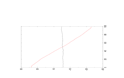
Figure 4: Shape of the string: below the transition the charged string is vertical. Above the transition it tilts away from the anisotropy axis.

Next we take into account thermal fluctuations. When the temperature is less than the activation energy of single angular kinks $\Delta E_{1}$, cf. (32), the line is rough as shown by Figure 5. Above $\Delta E_{1}$ single angular kinks are present in addition to the roughening, cf. Figure 2. The orientational order is then lost. These results clearly confirm what has been said in the previous sections. At temperatures higher than $\Delta E_{1}$, thermal fluctuations average the tilt angle to zero.

Figure 5: Rough inclined string at low temperature; orientational order is preserved.

V.2 Confinement regime

The same approach is performed in the confinement regime.

Figure 6 displays the absolute value of $\zeta$ as a function of $\gamma_{num}$. The behavior is the same as in the previous case. The straight string is stable below the transition and tilts above. However a jump in the order parameter is noticeable (especially in comparison with the equivalent Figure 3 concerning the elastic regime), an indication that the transition is first order. This is further confirmed by looking at the energy displayed on Figure 7. It is clearly discontinues as a function of $\gamma_{num}$ at the transition. The numerical study allows to capture the properties of the charged confined string in the whole range of $\gamma_{num}$. This is to be contrasted with the analytical work where we could not consider the small tilt angle region. In contrast with what has been said in teber this regime is not manifested by an instability of the string towards a modulation. The ground state given by the numerical simulations is also the straight, either inclined or not, string.

Figure 6: Absolute value of $\zeta$ as a function of $\gamma_{num}$ in the confinement regime.

Figure 7: Energy of the string as a function of $\gamma_{num}$. The solid line corresponds to the energy of a string. A discontinuity is clearly noticeable. The diamonds correspond to the first derivative of the latter.

At finite temperature the results for the confinement regime are qualitatively the same as for the elastic one.

VI Applications

VI.1 The solitonic lattice ($2D$)

The present study should be connected, as has been said in the Introduction, to the previous work on the statistical properties of solitons. Above, we have been considering the domain-line as given. Actually, in quasi-one dimensional systems, it has been shown in teber , with the help of a mapping to the ferromagnetic Ising model, that there are no strings, i.e. infinite domain lines of solitons, at non-zero temperature. The latter emerge from a process of exponential growth of aggregates of bisolitons below a crossover temperature $T_{cro}$. In the non-interacting case, $T_{cro}=T_{0}$ and the aggregates are finite rods perpendicular to the chains of the quasi-one dimensional system. At zero temperature the rods cross the whole system forming the free domain lines of solitons. In the interacting case the crossover temperature is lowered with respect to $T_{0}$ and becomes Coulomb dependent. In the region between $T_{0}$ and $T_{cro}$, intrachain antiferromagnetic interactions, within the ferromagnetic ground-state, take place in order for the bisolitons to aggregate, cf. teber . This is due to the important size-charging energy of the aggregates. A crucial approximation is that we have been neglecting shape instabilities in the interacting case. This reduced us to the region of the phase diagram where $\gamma_{D}<\gamma^{c}_{D}$, cf. (20). At high coupling constants, $\gamma_{D}\gg\gamma^{c}_{D}$, strings at $T=0$, or aggregates at finite temperatures should melt into a Wigner crystal of solitons. At intermediate coupling constants the present theory, dealing with shape instabilities should be relevant. It should be noted that in the previous paper we have suggested that shape instabilities give rise to a modulated string which would correspond to a single negative mode; as we have shown, the instability at intermediate coupling constant, is towards a tilt of the interface and affects a continuous set of modes.

We will first seek the stability of the string phase with respect to the Wigner crystal of solitons at $T=0$. Then we will concentrate on the non-zero temperature regime and look for the shape of the aggregates of solitons which lead to strings. To make comparison with the previous paper easier, notice that the present coupling constant, $\gamma=\gamma_{D}/\log l_{D}$, is similar to the coupling constant used in the previous paper $\Gamma$. Otherwise we have tried to preserve the same notations.

VI.1.1 Zero temperature results: from strings to Wigner crystal of solitons

We define $\gamma^{wc}_{D}$ as the coupling constant above which strings melt into a Wigner crystal at $T=0$. We would like to check here that $\gamma^{wc}_{D}>\gamma^{c}_{D}$ in order to preserve the coherence of the arguments.

As the Coulomb interaction increases, the string of solitons tilts. It’s energy also increases. This leads to a dissociation of the string as soon as it’s energy per soliton $\mu=\delta H^{(0)}/\delta N$ becomes larger than the energy of the constituent soliton $\mu_{sol}$. The latter corresponds to $2J_{\perp}R/a_{x}-(ze)^{2}/\epsilon R$ where $R\approx\sqrt{s/\nu}$ is the radius of the Wigner Seitz cell including the soliton and a background charge of density $\nu/s$ with $s=a_{x}a_{y}$. This energy can also be written as

$$\mu_{sol}=\frac{2J_{\perp}R}{a_{x}}\left[1-\nu\gamma\right]$$

where $\gamma$ is given by (18). The cohesion energy of the string is thus

$$E_{c}=J_{\perp}\left(\zeta+\frac{\gamma_{D}}{\sqrt{1+\zeta^{2}}}\right)-\mu_{sol}.$$ (37)

From (37) we see clearly that in the absence of Coulomb interaction, which implies that $\zeta=0$, the vertical string is stable. When the Coulomb interaction increases the tilt angle increases beyond the transition to the tilted phase. Thus $E_{c}$ increases from negative values. The melting of the string is given by $E_{c}=0$ and, $\zeta$ being the optimal angle of the string, (25). Starting with $\gamma_{D}\ll 1$ in $E_{c}=0$, (25) leads to the boundary $\gamma_{D}=1/\nu\gg 1$, in contradiction with the starting hypothesis. On the other hand, starting with $\gamma_{D}\approx 1/\nu$ leads to the lowest boundary $\gamma_{D}\approx\gamma_{D}^{*}$, cf. (26), again in contradiction with the starting hypothesis. The solution satisfying the self-consistent equation is thus in the intermediate coupling constant range $\gamma^{*}_{D}<\gamma^{wc}_{D}<1/\nu$ and is given by

$$\gamma^{wc}_{D}\approx 1/4\nu.$$ (38)

We see from (38), that for a sufficiently diluted system, $\gamma^{wc}_{D}\gg\gamma^{c}_{D}$, cf. (27). The tilted phase might thus be observed when this condition is satisfied.

VI.1.2 Non-zero temperature results: shape of the aggregates

More exotic is the non zero temperature case. From the point of view of interfaces, the latter roughen and thus collide at non-zero-temperatures. Equivalently, from the point of view of solitons there are no infinite lines but finite size aggregates. The size of the aggregates is approximately given by the distance between two successive collision points of neighboring interfaces. We address here the question of the shape of the charged aggregates of solitons in the intermediate regime where $\gamma^{c}_{D}<\gamma_{D}\ll\gamma^{wc}_{D}$. As has been said above, in this regime, the aggregates must adapt their shapes in order to minimize their electrostatic energy. An inclined aggregate, as in Figure 8 c), would thus be more favorable than the straight rod. But at finite temperature angular kinks are present and they further reduce the Coulomb energy. We can shown that a droplet with the lozenge shape of Figure 8 b) is favored in comparison with the previous aggregates. This is done by evaluating the energies of these aggregates $\Delta E_{b}=E_{b}-E^{(se)}_{b}$ and $\Delta E_{c}=E_{c}-E^{(se)}_{c}$ where their divergent self-energies $E^{(se)}_{b}$ and $E^{(se)}_{c}$ have been subtracted. For the aggregate c) the separation between the bikinks $x_{opt}$ is taken as the equilibrium separation under the combined action of the Coulomb force $(ze)^{2}/\epsilon x^{2}$ and the confinement one $-J_{\perp}/a_{x}$, i.e. $x_{opt}=\sqrt{s\gamma}$. Moreover, the tilt angle corresponds to the optimal one. In the confinement regime $\gamma$ is related to $\zeta$ with the help of (25). The regularized energies of the aggregates thus depend on one free parameter $\zeta$. The later must be larger than $1/\sqrt{2}$ to be in the stable confinement regime. We find that the difference between these energies $\Delta E_{c}-\Delta E_{b}>0$ as a function of $\zeta$ so that the energy of b) is always lower than that of c) above the critical coupling constant $\gamma^{c}_{D}$.

The results obtained in this section are summarized on the phase diagram Figure 9.

Figure 8: a) Rod in the absence of Coulomb interaction. The Coulomb energy of the lozenge b) is lower than that of c). At finite temperature the aggregates thus have the b) shape.

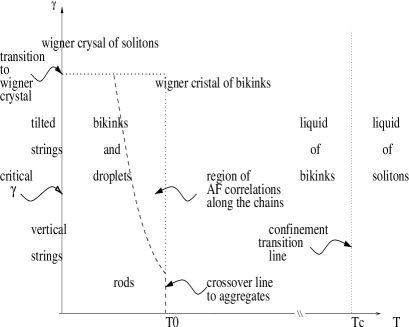
Figure 9: Phase diagram of the $2D$ system as a function of the coupling constant $\gamma_{0}$ and temperature $T$. Details are given in the text.

VI.2 The solitonic lattice ($3D$)

We consider briefly the important case of three dimensional systems where interfaces are domain walls. In $3D$ some rigorous statements allow a good understanding of the uncharged case in the frame of quasi-one dimensional systems, cf. bohr . In the presence of Coulomb interactions we shall thus follow bohr as well as our present experience of the charged $2D$ case. Concerning notations, in the third direction, $z$, the coupling constant will be taken as $J_{z}$ and the unit length as $a_{z}$.

VI.2.1 Uncharged domain wall

For the non-interacting case it has been shown in bohr that peculiarities are brought by the raise of dimensionality. In $3D$ the excitations analogous to rods would be disc-like objects. However, rigorous statements concerning the $3D$ case show that, at a temperature $T_{3}\approx 8J_{\perp}/\ln(2/\nu)\ll T_{c}\approx J_{\perp}/\nu$, a density $\nu_{c}=\nu-\nu_{n}$ of solitons condense into infinite anti-phase domain walls perpendicular to the chains of the quasi-one dimensional system; $\nu_{n}$ then corresponds to the density of finite size solitons below $T_{3}$. Therefore, the crossover regime of growing rods, which took place below $T_{0}$ in $2D$, cannot take place in $3D$ and is replaced by the transition at $T_{3}$.

The effect of thermal fluctuations on the walls is well known. Several authors have shown (see references in forgacs ) that, in $3D$ the hight-hight correlation function remains finite at $T<T_{R}$ whereas it diverges logarithmically for $T\geq T_{R}$, where $T_{R}>0$ is the roughening temperature. From these considerations $T_{3}$ may be considered as the roughening temperature. The existence of walls in $3D$ at finite temperatures is compatible with the fact that in Ising-like systems there is $2D$ long-range order at low temperatures.

VI.2.2 Charged domain wall versus Wigner crystal

The three-dimensional case of charged walls can be treaded the same way as the two-dimensional case. We will therefore consider again the elastic and confinement regimes. The Coulomb interaction will lead to a tilting of the wall here too. Two tilt angles can be defined now, because the anisotropy axis becomes an anisotropy plane. We will thus consider $\zeta_{y}$ which corresponds to the previous, in plane, tilt angle and $\zeta_{z}$ which is the tilt angle with respect to the third direction. The mean-field hamiltonian of the system is then

$$H_{p}/J_{y}=\zeta_{y}^{p_{y}}+\alpha_{\perp}\zeta^{p_{z}}_{z}+\gamma_{D}\left[\frac{1}{\sqrt{1+\zeta^{2}_{z}}}\left(1-\frac{1}{2}\log\left(\frac{1+\zeta^{2}_{y}}{1+\zeta^{2}_{z}}\right)\right)-1\right]$$ (39)

where, $\alpha_{\perp}=J_{z}/J_{y}$, $\gamma_{D}=e^{2}l_{D}/\epsilon s_{\perp}J_{y}$, $s_{\perp}=a_{y}a_{z}$ and in the last term, the contribution of the straight domain wall has been substracted. Notice that it is only in the case where $\zeta_{y}=\zeta_{z}=\zeta$ that we gain a global factor $1/\sqrt{1+\zeta^{2}}$ as in the $2D$ case. The logarithm is therefore the signature of a non-homogeneous charge dilatation within the wall.

Our aim is to determine the phase diagram, $\gamma_{D}$ versus $\alpha_{\perp}$ in both regimes, i.e. $p_{y,z}=1,2$. Among the four possible cases we will consider only the full elastic ($p_{y}=p_{z}=2$) and mixed ($p_{y}=2$, $p_{z}=1$) regimes.

In the elastic regime, $p_{y}=p_{z}=2$, the phase diagram is displayed on Figure 10. For $\gamma_{D}>2\alpha_{\perp}$, the stable solution is given by

$$\zeta_{y}=\zeta_{z}=0$$ (40)

In the region $\gamma_{D}<2\alpha_{\perp}$, the stable solution corresponds to

$$\zeta_{y}=0\qquad\zeta_{z}=\sqrt{\frac{\gamma_{D}}{2\alpha_{\perp}}-1}$$ (41)

For $\gamma^{s}_{D}\approx 16<\gamma_{D}<(2\alpha_{\perp})^{3/2}\sqrt{\log\alpha_{\perp}/4}$ a third phase, corresponding to

$$\zeta_{y}\approx\left(\frac{\gamma_{D}}{6}\log\left(\frac{\gamma_{D}}{4}\right)\right)^{1/3}\qquad\zeta_{z}=0$$ (42)

is stable. The domain of validity of this solution overlaps the ones of the two previous solutions. With the help of energetic considerations, we find that a line of first order critical points, at $\gamma_{D}\approx 20$, separates phase (40) from phase (42). By the same way, a line of first order critical points has been found to separate phase (41) from phase (42). The line $\gamma_{D}=2\alpha_{\perp}$ is a line of second order critical points which terminates at the critical end-point $\alpha_{\perp}=10$, $\gamma_{D}=20$. Phases which would have both angles none-zero appeared to be unstable.

Figure 10: Phase diagram of the elastic wall: $\gamma_{D}$ as a function of $\alpha_{\perp}$.

A similar analysis can be done for quasi-two dimensional ($Q2D$) systems where the interface is elastic within the planes, i.e. $p_{y}=2$ and in the confinement regime between planes, i.e. $p_{z}=1$. For $Q2D$ systems, the coupling in the third direction is weak with respect to the coupling in other directions, i.e. $\alpha_{\perp}<1$. In the region of the phase diagram where $\alpha_{\perp}<1$ the solution is thus given by

$$\zeta_{y}=0\qquad\zeta_{z}=\frac{\gamma_{D}}{2\alpha_{\perp}}+\sqrt{\left(\frac{\gamma_{D}}{2\alpha_{\perp}}\right)^{2}-1}$$ (43)

and is stable for $\gamma_{D}>2\alpha_{\perp}$. As before, when $\gamma_{D}<2\alpha_{\perp}$, the untilted solution is stable for small $\alpha_{\perp}$ and is separated from the previous by a line of second order critical points. From (41) and (43), we see that for a given value of the ratio $\gamma_{D}/2\alpha_{\perp}$, the tilt is stronger in the mixed regime than in the pure elastic regime. This can be interpreted by considering the equilibrium position of a constituent of the wall due to the constant confinement force and the constant electric force due to the charged wall; a priori, the equilibrium is reached only at $\gamma_{D}=\alpha_{\perp}$, a feature which is peculiar to the confinement regime. This implies that the wall should melt as soon as $\gamma_{D}>\alpha_{\perp}$ or, if the Coulomb energy scale is sufficiently weak, that the wall should strongly incline to reduce the coupling constant. Allowing the wall to tilt, the equilibrium equation, $\gamma_{D}=\alpha_{\perp}$, is generalized to

$$\frac{\gamma_{D}}{\alpha_{\perp}}\left(1-\frac{1}{2}\log\left(1+\zeta^{2}_{z}\right)\right)=1.$$

which leads to the following minimal stability angle

$$\zeta_{z}=\exp\left(2\left(1-\frac{\alpha_{\perp}}{\gamma_{D}}\right)\right)-1.$$

above which the wall stabilizes at the equilibrium angle (43).

In $3D$, the situation is thus richer than in the $2D$ case with the appearance of a tricritical point and quantitative differences between the various regimes but, qualitatively, the same phase diagram for all of them. In particular, the tilting of the interface takes place with respect to a single anisotropy axis and not both. In quasi-two dimensional systems, the wall should tilt with respect to the third direction rather than $y-$direction and the tilting is stronger in the confinement regime to prevent the melting. Another difference with the $2D$ case is that thermal fluctuations do not affect these results, as long as we are below the roughening temperature of the wall.

VI.3 Stripes in oxides

Up to know the whole theory is model independent. As we have already mentioned our results could be applied to doubly commensurate charge-density waves such as polyacetylene. We will however consider physical systems which are quite extensively studied nowadays. These are the oxides, e.g. cuprate, nickelate, manganese and the new ferroelectric state. The latter will be considered in the next section. We will focus here on the phenomenology of stripes with the help of the above theory. We concentrate only on the long distance properties, namely, the fact that stripes consist of lines or walls of holons which are similar to the charged solitons we have been considering. The latter are thus charged interfaces as the ones described in this paper.

The oxides we consider are quasi-two dimensional materials formed by coupled planes. At intermediate values of doping, a $3D$ ordering of the stripes might have been seen in $La_{1.6-x}Nd_{0.4}Sr_{x}CuO_{4}$ and $La_{2-x}Sr_{x}NiO_{4+\delta}$, cf. Tranq and references therein. The impact of the pinning by the lattice and the Coulomb interactions play a crucial role in these systems.

In $La_{1.6-x}Nd_{0.4}Sr_{x}CuO_{4}$ neutron diffraction studies have revealed diffuse magnetic peaks along the $z$-direction, in the stripe phase, which is consistent with stripes as one-dimensional interfaces. Moreover, $X$-ray studies reveal that stripes are parallel in next-nearest-neighboring layers but orthogonal between nearest layers. This $3D$ ordering is probably due to a pinning of the stripes by the lattice structure.

The case of nickelates is more interesting. In $La_{2-x}Sr_{x}NiO_{4+\delta}$ there is a body-centered stacking of parallel elastic stripes with only weak perturbations due to the lattice. This $3D$ ordering is due to Coulomb repulsion and might correspond to a domain wall with a step-like profile suggesting a confinement regime in the third direction. This justifies the mixed confinement-elastic regime we have considered in VI.2. Experimental results do not however exclude the interpretation of this $3D$ ordering as a Wigner crystal of lines. The latter hypothesis allows us to focus on strings within planes of the quasi-two dimensional system, as we are going to do in the next paragraph.

Following Wakimoto & al incli , we are going to recall briefly here some experimental results related to the tilting of string-like stripes in $La_{2-x}Sr_{x}CuO_{4}$.

The experimental results are summarized on Figure 11 which has been taken from incli . In Figure 11 (a), $\delta=2\pi/d$ where $d$ is the distance between stripes. At low doping, the inset on the left of this figure, shows magnetic Bragg peaks corresponding to a one-dimensional spin modulation which is inclined with respect to the reference tetragonal axis. At higher doping, the inset on the left, shows that this spin modulation, along with the charge stripes, have rotated by an angle of $45$ degrees. The main figure, together with Figure 11 (b) which displays the tilt angle as a function of the concentration of dopant, show that this shape instability takes place around $x_{c}\approx 0.05$ where $\delta$ increases linearly with $x$. Moreover, the authors report a weak dependence of the magnetic peaks on the third direction. This implies that the spin modulations are weakly correlated between successive $CuO_{2}$ layers. Thus, the stripes can be considered with a good accuracy as charged strings which justifies our starting hypothesis.

The stripe instability observed experimentally might be due to the competition between the long-range Coulomb interaction and an anisotropic interaction. To relate this instability to an increase of the concentration of dopants $x$ we should probably take into account structural changes. As argued by Tranquada & al Tranq , the lines of charge might be pinned along the direction of the tilt of the $CuO_{6}$ octahedron. This tilt direction varies with doping. It is along the orthorhombic axis at low doping and along the tetragonal axis at higher doping. These axis are $45$ degrees from each-other. At an intermediate doping, corresponding to the critical value $x_{c}$, a $45$ degrees tilt of the stripes, satisfying the structural constraints, can take place.

Simple considerations related to the competing energy scales are in favor of such an order of magnitude for the tilt angle. First, in this system $e^{2}/\epsilon a\sim 0.1-1eV$ where $a$ is a unit length of the tetragonal structure. Second the exchange energy $J_{\perp}$ is of the order of $0.13eV$. Thus $\gamma\sim 0.4-4.5$ where (18) has been used. If we consider that the Debye length is of the order of the inter-stripe distance $1/\delta$, at the transition $x_{c}$ we have $l_{D}\sim 20a$. Thus $\gamma_{D}=\gamma\ln(l_{D}/a)\sim 1.2-13.5$. Using (21), the maximum tilt angle compatible with these values is around $55$ degrees. A tilt angle of $45$ degrees can be reached with a $\gamma_{D}\sim 4.0$ which is clearly in the range of allowed values above. Hence, the competing interactions can be responsible for such a tilt.

This tilt could reduce the electrostatic energy of the stripe as can be seen by the following argument. At low doping, i.e. in the diagonal stripe phase, the hole concentration along the stripe is $0.7$ hole/Cu. This concentration is reduced to $0.5$ hole/Cu in the collinear stripe phase, cf. Wakimoto & al. The density of charges along the stripe is thus reduced by $\sqrt{1+\zeta^{2}}$, with $\zeta=1$ for the present $45$ degrees tilt angle. This dilatation factor reduces the electrostatic energy of the string as has already been seen in (19). This could hold assuming that the number of holes$/$stripe is constant. The added dopants would lead to the formation of new stripes. The latter become tightly packed at high doping as suggested by the linear relation $\delta\approx x$.

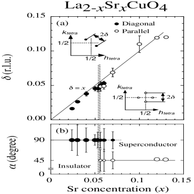
Figure 11: Tilting of stripes in a cuprate oxide (from incli ).

VI.4 Uniaxial ferroelectrics

Recently a ferroelectric Mott-Hubbard state has been observed in quasi 1D organic superconductors such as $(TMTTF)_{2}X$. We give a brief account on the origin of this phase and connect the results to our present study. Experimental and theoretical results are given in detail in Monceau .

In the system mentioned above $TMTTF$ are molecules composing the stacks and therefore giving rise to the one dimensional nature of the compound. $X$ are ions placed in the vicinity of the molecules. At large temperatures, of the order of $100K$, the ions reorder through a uniform shift which gives rise to a ferroelectric phase. The latter has been detected via the measurement of the dielectric susceptibility which shows a gigantic anomaly at low frequency around $T_{fe}\sim 150K$. At low temperature domain lines, separating domains with opposite polarization, should be observed. Their existence is necessary to minimize the external electric field generated by charges accumulating at the boundary of the sample. Moreover, as the interface corresponds to a jump in the polarization it is charged. Following Monceau we shall define as $\alpha-$solitons the elementary constituents of the interface which connect domains with opposite polarization. They carry a fractional charge $ze$ with $z=2\alpha/\pi$.

Two facts suggest that this system is a good candidate for the observation of charged interfaces. First the background dielectric susceptibility $\epsilon_{0}\sim(\omega_{p}/\Delta)^{2}\sim 10^{4}$ is large. Further more $\pi-$solitons are also present and they screen the Coulomb interaction. This weakens the Coulomb interaction. In such systems, the strings of $\alpha-$solitons should thus be stable against a melting towards a Wigner crystal. Bubble-like aggregates of $\alpha-$solitons, as the ones described in VI, could also be observed at higher temperatures.

VII Conclusion

The statistical properties of charged interfaces, strings and walls, has been studied. We have found that shape instabilities, due to competing interactions, play a fundamental role. They manifest themselves through zero-temperature phase transitions from which new ground-states emerge where the interface is tilted. The $2D$ case of the string has been extensively studied. For small tilt angles the string is elastic and the transition to the tilted ground state is second order. On the other hand a first order transition takes place if we are beyond the limit of validity of the elastic regime, i.e. in the confinement regime. At non-zero temperatures it has been shown that in either regimes a pure Coulomb roughening of the string, due to the proliferation of angular-bikinks, exists in addition to the usual roughening as soon as $T>0$. At higher temperatures angular-kinks are thermally activated and connect the degenerate ground-states. These results have been confirmed with the help of a numerical approach based on the Monte Carlo - Metropolis algorithm. We have then related the present study to the general problem of the statistical properties of solitons in charge-density wave systems in either $2$ or $3$ dimensions. In $2D$ systems the string has been shown to emerge from lozenge-like aggregates of solitons upon decreasing temperature. In $3D$, the additional coupling constant in the third direction enriches the tilted phases with the appearance of a tricritical point separating them. In the confinement regime, a disintegration of the wall is favored but the solitons might order in the form of a strongly inclined wall. Applications concerning stripes in oxides and a possible explanation of their tilt, as well as charged strings in uniaxial ferroelectric experiments, have also been considered.

Aknowledgments

I would like to thank S. Brazovskii for helpful and inspiring discussions from the very beginning of this work. I would like to thank A. Bishop for discussions and his hospitality at the Theoretical Division and Center of Non-Linear Studies, of Los Alamos.

Appendix A

In this appendix we give some details on the screening in the ensemble of solitons. Screening makes the energy extensive and gives a meaning to the thermodynamic limit as has been said all along the paper. In the following we will work in the RPA approximation which is very well known in the field on many-body theory. This allows us to derive the Debye length and the electrostatic potential in two cases: two and three-dimensional screening.

We consider first a single plane embedded in $3D$ space. This case corresponds to two-dimensional screening. Supposing the Coulomb field $\phi$ slowly varying, it obeys the following semi-classical equation

$$-\epsilon\Delta\phi(\overrightarrow{R})=-4\pi e^{2}(\Pi^{(0)}*\phi)(\overrightarrow{R})\delta(z)+4\pi e^{2}\rho_{0}(\overrightarrow{r})\delta(z)$$ (44)

where $\overrightarrow{R}$ is a $3D$ vector associated with the $3D$ Coulomb field, $\overrightarrow{r}$ is a $2D$ vector indexing the charges which are embedded in the $z=0$ plane and $\rho_{0}$ is some external charge. $\Pi^{(0)}(x,y)$ is the response function, or polarization part, of the soliton system which is related to the correlation function by fluctuation dissipation theorem

$$T\Pi^{(0)}(\overrightarrow{r})=<\delta\rho(\overrightarrow{r})\delta\rho(\overrightarrow{0})>$$ (45)

where $\delta\rho(\overrightarrow{r})=\rho(\overrightarrow{r})-\nu$, $\rho(\overrightarrow{r})$ being the density of solitons and $\nu$ the background neutralizing charge.

The first term on the right of (44) corresponds to the screening charge. This term implies linear screening and dispersion via the convolution. The Coulomb field is then

$$\phi(\overrightarrow{k},z=0)=\frac{2\pi e^{2}\rho_{0}(\overrightarrow{k})}{\epsilon|k|+2\pi e^{2}\Pi^{(0)}(\overrightarrow{k},z=0)}$$ (46)

where $\overrightarrow{k}$ is the reciprocal vector associated with $\overrightarrow{r}$. The fact that the potential is evaluated at $z=0$ implies that the field lines are confined to the same space as the particles, cf. Cornu . Expression (46) leads to the Debye screening of the field with a Debye length

$$\frac{1}{l_{2D}}=\frac{2\pi e^{2}}{\epsilon}\Pi^{(0)}(k=0).$$ (47)

Also the $k-$term in the denominator of (46) is a feature of $2D-$systems. In real space this leads to an algebraic screening instead of the exponential one, cf. Cornu for detailed studies of screening effects in Coulomb fluids and below for an example.

We consider now the three dimensional case of independent planes embedded in a neutral media. Such a system of decoupled planes brings a $3D-$screening. The screening charge is then a function of the three-dimensional vector $\overrightarrow{R}$. But, as the planes are independent, the bare correlation function corresponds to $\Pi^{(0)}(\overrightarrow{R})=\Pi^{(0)}(\overrightarrow{r})\delta(z)$. By the same arguments as in the first section we can compute the coulomb field which reads

$$\phi_{3D}(\overrightarrow{K})=\frac{4\pi e^{2}\rho_{0}(\overrightarrow{K})}{\epsilon K^{2}+4\pi e^{2}\Pi^{(0)}(\overrightarrow{k},z=0)/a_{z}}$$ (48)

where we consider only the $z=0$ plane subject to the bulk screening. The three-dimensional Debye length is then given by

$$\frac{1}{l^{2}_{3D}}=\frac{4\pi e^{2}}{\epsilon a_{z}}\Pi^{(0)}(k=0)$$ (49)

where $a_{z}$ is the inter-plane distance. In real space (48) leads to the usual exponential screening.

Finally we derive the polarization part for the present problem. This gives explicit expressions for the screening lengths and for $\phi(\overrightarrow{r})$. Below the crossover transition $T_{0}$

$$T\Pi^{(0)}(x,y)\approx\frac{1}{2s^{2}}\nu a_{x}\exp\left(-\frac{2y}{l_{\perp}}\right)\left(2\delta(x)+\delta(x+a_{x})+\delta(x-a_{x})\right)$$ (50)

corresponding to the aggregation of the solitons into rods of length $l_{\perp}$, cf. bohr . Fourier transforming (50) we get

$$T\Pi^{(0)}(\overrightarrow{k})\approx\frac{\nu}{4sa_{y}}(1+\cos(k_{x}a_{x}))\frac{l_{\perp}}{1+k^{2}_{y}l^{2}_{\perp}/4}.$$

Thus $\Pi^{(0)}(\overrightarrow{k})\approx\frac{\nu l_{\perp}}{2sa_{y}T}$ and, as we work at constant density of solitons $\nu$, $l_{\perp}\approx\sqrt{2\nu}\exp(2J_{\perp}/T)$. With the help of (47) and (49), this yields

$$l_{2D}=\frac{2\epsilon sa_{y}T}{\pi e^{2}(2\nu)^{3/2}}\exp\left(-\frac{2J_{\perp}}{T}\right),$$

$$l_{3D}=\sqrt{\frac{\epsilon sa_{z}T}{\pi e^{2}(2\nu)^{3/2}}}\exp\left(-\frac{J_{\perp}}{T}\right).$$ (51)

In the $2D-$screening regime, the field can then be written, in the long distance limit with respect to the coarse graining length $a_{x}$

$$\phi(\overrightarrow{k})=\frac{2\pi e^{2}}{\epsilon}\frac{1+k^{2}_{y}l^{2}_{\perp}/4}{|k|(1+k^{2}_{y}l^{2}_{\perp}/4)+1/l_{D}}$$ (52)

which reflects the anisotropy of the problem. To give an idea of the algebraic screening we Fourier transform (52) in the limit $k_{y}l_{\perp}\rightarrow 0$, i.e. far enough from the rod. This yields

$$\phi(\overrightarrow{r})\approx\frac{2\pi e^{2}}{\epsilon}\frac{l_{D}^{2}}{r^{3}}$$

in the limit $r\gg l_{D}$. We see that the algebraic tail leads to a slow decay of the potential in contrast to the usual exponential one. However this type of interaction, of the dipolar-type, beyond the screening length are compatible with the growth of the aggregates, cf. teber . For more details on the peculiar screening properties of such system with anisotropic intrinsic charges see these .

Appendix B

Our purpose is mainly to show the differences and common points between the two interface models. The approach is based on the transfer matrix technic. In the present case, this formulation cannot be used straight forwardly because of the long-range interactions in (10). Some results obtained in the non-interacting case should however remain in the presence of the long range interaction. It is on such a property that we focus now.

The associated Hamiltonian of the problem is

$$\beta H_{p}=\frac{K}{a^{p-1}}\sum^{L-1}_{y=0}|x_{y+1}-x_{y}|^{p}$$ (53)

where the short distance cut off has been taken explicitly into account. The transfer matrix $\widehat{T_{a}}$ is defined as an integral operator with eigenfunctions $\psi(x)$ whose kernel is expressed in terms of (53). Namely

$$\widehat{T_{a}}\psi(x)=\int dx^{\prime}\exp\left(-\frac{K}{a^{p-1}}|x-x^{\prime}|^{p}\right)\psi(x^{\prime}).$$ (54)

The free problem is simple enough to be treated just with the integral equation (54). For a more exhaustive account on the general results one can obtain with help of the transfer matrix technic see suris .

For both models the eigenfunctions of the transfer matrix are simply plane waves

$$\psi_{k}(x)\approx\exp(ikx).$$

This amounts to Fourier transform the kernel of (54). The eigenvalues of the transfer matrix associated to both interface models are thus

$$\epsilon^{G}_{k}\approx\frac{k^{2}}{2K}\qquad\qquad\epsilon^{SOS}_{k}\approx\log\left(K^{2}+k^{2}\right).$$ (55)

By comparing the two spectrums in (55) we see clearly that both models have the same long distance, i.e. $k\rightarrow 0$, properties.

References

- (1) S Brazovskii and N Kirova 1984 Physics (Soviet Scientific Reviews Section A) vol 5, ed I M Khalatnikov (New York: Harwood Academic) p 99
- (2) Yu Lu, Solitons and Polarons in Conducting Polymers, World Scientific Publ. Co., 1988
- (3) A J Heeger, S Kivelson and J R Schrieffer Rev. Mod. Phys. 60 (1988) 781
- (4) P Monceau, F Ya Nad and S Brazovskii, Phys. Rev. Lett. 86 (2001) 4080
- (5) Tranquada J M, 1998, Neutron Scattering in Layered Copper Oxide Superconductors, ed A Furrer (Dordrecht: Kluwer)
- (6) M Bosch, W van Saarloos and J Zaanen, Phys. Rev. B 63 (2001) 092501
- (7) S Wakimoto & al Phys. Rev. B 61 (2000) 4326; M Fujita, K Yamada & al. Phys. Rev. B 65 (2002) 064505
- (8) P Dai & al. Phys. Rev. Lett. 85 (2000) 2553
- (9) J H Schon, S Berg, Ch Kloc and B Battlogg 2000, Science 287 1022
- (10) T Bohr and S Brazovskii, 1983, J. Phys. C: Solid State Phys 16 1189
- (11) S Teber, B P Stojkovic, S A Brazovskii and A R Bishop, J. Phys.: Condens. Matter 13 (2001) 4015-4031
- (12) Y. Kantor & M. Kardar, Europhys. Lett. 9 (1989) 53
- (13) R. Netz & H. Orland, Eur. Phys. J. B 8 (1999) 81
- (14) P A Lee, T M Rice and P W Anderson, Solid State Comm. 14 (1974) 703
- (15) M J Rice, A R Bishop, J A Krumhansl and S E Trullinger 1976 Phys. Rev. Lett. 36 432
- (16) G Forgacs & al Phase Transitions and Critical Phenomena vol 14 (1991) ed C Domb and J L Lebowitz (London: Academic)
- (17) F Cornu, Thèse d’habilitation (1998); F Cornu, 1996, Phys. Rev. E., 53, 4595; B Jancovici, 1995, J. of Stat. Phys, 80, 445
- (18) R A Suris Soviet. Phys. JETP 20 (1965) 961
- (19) S. Teber, Thèse de doctorat (2002)