Orientational and induced contributions to the depolarized Rayleigh spectra
of liquid and supercooled ortho-terphenyl

Abstract

The depolarized light scattering spectra of the glass forming liquid ortho-terphenyl have been calculated in the low frequency region using molecular dynamics simulation. Realistic system’s configurations are produced by using a recent flexible molecular model and combined with two limiting polarizability schemes, both of them using the dipole-induced-dipole contributions at first and second order. The calculated Raman spectral shape are in good agreement with the experimental results in a large temperature range. The analysis of the different contributions to the Raman spectra emphasizes that the orientational and the collision-induced (translational) terms lie on the same time-scale and are of comparable intensity. Moreover, the cross terms are always found to be an important contribution to the scattering intensity.

I INTRODUCTION

Depolarized light scattering (DLS) spectroscopy has been proved to be a valuable tool to explore the dynamical properties of molecular fluids Pecora76 . In the case of supercooled and glass forming liquids, DLS has been used by several researchers with the aim to elucidate the dynamical mechanisms underlying the liquid-glass transition Tao91 ; Li92 ; Du94 ; Wuttke94 ; Pick94 ; Lebon95 ; Alba95 . However, the uncertainties in the scattering mechanisms giving rise to the Raman spectra, and the consequent hypotheses that have been introduced to interpret the experiments, leave open the problem of a reliable analysis.

In some glass forming liquids, DLS spectra have been interpreted as arising primarily from interaction-induced mechanisms — namely dipole-induced-dipole (DID) — and so they have been related directly to the dynamics of the density fluctuations and compared with the outcomings of mode-coupling theories (MCT) Goetze92 . Following this line, Cummins et al. Li92 have interpreted the spectra of salol as arising entirely from the DID mechanism; in a more recent work Cummins96 , however, the authors assume that orientational contributions dominate the DLS spectra of salol at least up to $4000$ GHz, and the connection with the density fluctuations dynamics has to rely on a strong coupling between rotational and translational degrees of freedom. The situation is similar also for other systems. In the case of an other prototype of fragile glass-forming liquid, the ortho-terphenyl (OTP), Patkoswski et al. Pecora97 state that the low frequency part of the spectrum, up to about $10$ GHz, is due to collective reorientation, while at higher frequency the DID contribution is dominating.

We think that a careful investigation of the scattering mechanisms which contribute to DLS spectra is needed in order to clarify what type of information is possible to extract from the experimental data, and to ascertain the connections with the density fluctuation correlators treated by MCT.

In the present work we investigate the low frequency DLS spectra of liquid OTP for temperatures above and close to the MCT critical temperature $T_{c}$. We use the new realistic intra- and inter-molecular potential model set up by some of us very recently Mossa00 ; Mossa01 ; soundwaves ; fast . Various single particle correlation functions have already been studied through classical molecular dynamics (MD) simulations, yielding noticeable results. It is now possible to combine realistic dynamical configurations with plausible polarizability models, and try to discriminate among the different hypotheses on the origin of the different contributions to DLS experimental spectra.

The paper is organized as follows: Sec. II is a brief recall of our potential model and of the methods used to produce the dynamical configurations. In Sec. III we recall the main polarizability models that have been used so far to calculate the DLS spectra of simple molecular liquids; moreover, we show how they can be used to estimate the DLS spectra for our realistic flexible model. The computational details are treated in Sec. IV, while the results and a discussion are presented in Sec. V. In Sec. VI we address some conclusions.

II THE MOLECULAR MODEL

In our flexible model Mossa00 the OTP molecule is constituted by three rigid hexagons (phenyl rings) of side $L_{a}=0.139$ nm. Two adjacent vertices of the parent (central) ring are bonded to one vertex of the two side rings by bonds whose length at equilibrium is $L_{b}=0.15$ nm. Each vertex of the hexagons is thought to be occupied by a fictious atom of mass $M_{CH}=13$ a.m.u. representing a carbon-hydrogen (C-H) pair. In the isolated molecule equilibrium configuration, the two lateral rings lie in planes that form an angle of about 54^o with respect to the central ring’s plane. The three rings of a given molecule interact among themselves by an intramolecular potential $V_{intra}$. This potential is chosen in such a way to preserve the molecule from dissociation, to give the correct relative equilibrium positions for the three phenyl rings, and to represent at best the isolated molecule vibrational spectrum. In particular, it is written in the form $V_{intra}=\sum_{k}c_{k}V_{k}({\bm{r}})$, where each term $V_{k}({\bm{r}})$ controls a particular degree of freedom; the actual values of the coupling constants $c_{k}$ have been determined in order to have a realistic isolated molecule vibrational spectrum. Several internal motions have been taken into account, like the stretching along the ring-ring bonds and between the side rings, and the rotation of the lateral rings along the ring-ring bonds.

The intermolecular part of the potential, concerning the interactions among the rings pertaining to different molecules, is described by a site-site pairwise additive Lennard Jones (LJ) $6-12$ potential, each site corresponding to one of the six hexagons vertices. The details of the intramolecular and intermolecular interaction potentials, together with the values of the potential parameters, are reported in Ref. Mossa00 .

It is worth noting that previous studies of the temperature dependence of the self diffusion constant Mossa00 and of the structural ($\alpha$) relaxation times Mossa00 ; Mossa01 , indicate that this model is capable to quantitatively reproduce the dynamical behavior of the real system, but the actual simulated thermodynamical point has to be shifted by $\approx$ 20 K upward. In the following, when we compare the simulation results with the experiments, the reported MD temperatures are rescaled by such an amount.

III POLARIZABILITY MODELS

In a liquid composed of $N$ optical anisotropic units (a unit can be the entire molecule, a group of atoms in the molecule, or a single atom inside the molecule), characterized by a permanent polarizability tensor ${\bm{\alpha}}$, the classical low frequency DLS spectrum in the dipole approximation is proportional — apart from a trivial frequency factor — to the Fourier transform of the time correlation function of the traceless tensorial part ${\bm{\Pi}}_{2}$ of the collective polarizability ${\bm{\Pi}}$. ${\bm{\Pi}}$ can be approximated by the sum of two terms: the first, ${\bm{\Pi}}^{M}$, is the sum of all the permanent polarizabilities dependent on the orientational variables ${\bm{Q}}_{i}$ of the units; the second, ${\bf\Pi}^{I}$, is due to all the interaction induced contributions, and its leading part can be written in term of the dipole propagator tensor ${\bm{T}}^{(2)}(i,j)={\bm{\nabla}}^{2}R_{ij}^{-1}$ (where $R_{ij}$ is the distance between the i-th and j-th units):

$${\bm{\Pi}}={\bm{\Pi}}^{M}+{\bm{\Pi}}^{I}$$ (1)

$${\bm{\Pi}}^{M}=\sum_{i}\left\{{\bm{\alpha}}_{i}({\bm{Q}}_{i})\right\}=\sum_{i}(\alpha{\bm{1}}+\frac{2}{3}\gamma{\bm{Q}}_{i})$$ (2)

$${\bm{\Pi}}^{I} = \sum_{i}{\sum_{j}{{\bm{\alpha}}_{i}{\bm{T}}^{(2)}(i,j){\bm{\alpha}}_{j}}}$$

$$+ \sum_{i}\sum_{j}{\sum_{k}{\bm{\alpha}}_{i}{\bm{T}}^{(2)}(i,j){\bm{\alpha}}_{j}{\bm{T}}^{(2)}(j,k){\bm{\alpha}}_{k}}$$

$$+ \ldots$$

Here ${\bm{\Pi}}^{M}$ is written for units with symmetric top symmetry, $\alpha$ and $\gamma$ are the isotropic and anisotropic polarizabilities, and ${\bm{Q}}_{\alpha\beta}=(3/2){\bf\hat{u}}_{\alpha}{\bf\hat{u}}_{\beta}-(1/2){\bm{\delta}}_{\alpha\beta}$, where ${\bf\hat{u}}$ is a unit vector along the symmetry axis.

Usually only the first order DID is considered in Eq. (III), the second order DID being sometimes completely disregarded. The relative importance of the higher order DID contributions with respect to the first one is dependent on the strength of the permanent polarizability tensor, and on the minimum approach distances of the units Birnbaum85 . However, it is well known from the study of noble gas systems, that at short distances, when high order contributions become important, also other multi-pole and quantum electron correlation effects have to be considered. These terms are usually found to be of opposite sign respect to the DID contribution Dacre82 ; Hunt85 . Empirical diatomic induced polarizabilities have negative corrections at short distances for all noble gases Barocchi85 , and only for gaseous mercury a small positive correction to the second order DID has been used to fit the experimental spectra Sampoli95 . From these considerations, in the present work we discuss only the contributions from the first and second order DID.

We want to underline that, in the case of OTP, the choice of the unit is not so obvious as for monatomic fluids or simple molecular fluids such as $N_{2}$. Thus, the subsequent choices are based on the following considerations. Even for simple molecular systems, like $CO_{2}$ or $CS_{2}$ fluids, we can consider as unit the entire molecule, each atom, or the peripheral (most polarizable) atoms. In the case more units are pertaining to the same molecule, these units are at short distance each other, so their induced contributions are tentatively treated in a more refined scheme. The major attempt in this way has been made by Applequist Applequist72 . His formalism, introduced to reproduce the molecular polarizabilities with transferable atomic polarizabilities, is equivalent to take into account the DID at all orders. Indeed the distances are so short that the major contributions come from higher order DID interactions. Irrespective to the relative success of the method, various authors Olson78 ; Thole81 ; Applequist93 have modified the scheme adding mono-pole polarizability, and/or using non isotropic atomic polarizability, and/or separating atoms of the same species on the base of chemical bonds. Only a few attempts have been made so far to use the Applequist formalism to calculate the experimental spectra Birnbaum85 , and with doubtful improvements. Thus, at present we are not confident in using classical dipole interactions at short distances.

So far we have not tried to use a complex polarizability scheme for our molecular model, and we have chosen to adopt two models that can give a rough estimate of a lower and upper limit of the induced interactions. In our potential model, three six sites rigid rings form the molecule and this suggests to consider as units the rings themselves (R scheme), or the six sites of each ring (S scheme). We have always neglected the effects on the polarizability due to the change of one (or two) H-C with a C-C bond. In the R scheme, the polarizability tensor is taken equal to that of benzene ($C_{6}H_{6}$). In the S scheme, we have simply divided by six the polarizability tensor of benzene, and we have neglected the DID contributions coming from atoms pertaining to the same ring. The induced contributions grow up at least with the sixth power of the inverse of the distance, so we expect the R scheme to be a lower limit to the induced contributions, while the S scheme to be an upper one. Indeed, in the S scheme the mean distances are shorter than in R scheme. We want to underline that, if in the S scheme the DID interactions inside the ring were taken into account, this would have reduced the polarizabilities of the six sites.

Using a notation similar to that of Stassen et al. Ladanyi94 , we can work out the collective polarizability correlation function for the depolarized scattering:

$$C(t)=\frac{1}{10V}\langle{\bm{\Pi}}_{2}(t){\bm{:}}{\bm{\Pi}}_{2}(0)\rangle,$$ (4)

where $V$ is the volume occupied by the $N$ units. $C(t)$ can be divided in three terms, namely the orientational term $C_{or}(t)$, the interaction-induced or DID term $C_{ii}(t)$, and the cross contribution term $C_{cr}(t)$:

$$C(t)=C_{or}(t)+C_{ii}(t)+C_{cr}(t),$$ (5)

with

$$C_{or}(t) = \frac{2}{45V}\gamma^{2}\langle{\bm{Q}}(0){\bm{:}}{\bm{Q}}(t)\rangle$$

$$C_{ii}(t) = \frac{1}{10V}\langle{\bm{\Pi}}_{2}^{I}(0){\bm{:}}{\bm{\Pi}}_{2}^{I}(0)\rangle$$ (6)

$$C_{cr}(t) = \frac{1}{15V}\gamma\left[\langle{\bm{Q}}(0){\bm{:}}{\bm{\Pi}}_{2}^{I}(t)\rangle+\langle{\bm{\Pi}}_{2}^{I}(0){\bm{:}}{\bm{Q}}(t)\rangle\right].$$

Here ${\bm{Q}}=\sum_{i}{{\bm{Q}}_{i}}$ and all the sums are extended over the $N$ units.

Although the importance of the three terms in Eq. (6) has been found similar in various systems Birnbaum85 , the cross term $C_{cr}(t)$ has been neglected, without sound arguments, in various works on glass-forming liquids. The integrated intensities of the orientational contribution, i.e., the value at $t=0$ of the correspondent correlation function, can be written as:

$$C_{or}(t=0)=\frac{N}{15V}\gamma^{2}(1+f_{2}),$$ (7)

where $g_{2}=1+f_{2}$ is the static angular pair correlation factor between our units, defined as Gershon69

$$g_{2}\equiv\frac{2}{3N}\sum_{i}\sum_{j\neq i}\langle{\bm{Q}}_{i}(0){\bm{:}}{\bm{Q}}_{j}(0)\rangle.$$ (8)

It is well known that, if the units are spherically symmetric ($\gamma=0$), the orientational and cross contributions do vanish, as in the case of DLS from monatomic fluids. In both R and S schemes, we expect a value of $g_{2}$ rather different from $1$. Indeed, also in the R scheme we have a strong orientational correlation between different units (rings pertaining to the same molecule). This is quite different from the case of simple molecular fluids, such as $N_{2}$, where only very small orientational correlations exist between different molecules, even in the liquid phase near the melting point. If all the rings of OTP molecules were in the equilibrium positions, while there was no correlation between the orientation of different molecules, we can calculate the $g_{2}$ factor for both R and S models. Using the equilibrium values of the cosines between the normals to the ring planes (${\bf n}_{1}\cdot{\bf n}_{2}={\bf n}_{1}\cdot{\bf n}_{3}=0.588$, and ${\bf n}_{2}\cdot{\bf n}_{3}=0.673$, with the index $1$ standing for the central ring Mossa00 ), we have

$$g_{2}^{R,eq}\approx 1.14,\;\;g_{2}^{S,eq}=6\times g_{2}^{R,eq}\approx 6.84.$$ (9)

Obviously, the obtained $g_{2}$ factors make the orientational contribution integrated intensity — in this idealized condition — independent of the adopted scheme. Since the relation $g_{2}^{R,eq}=g_{2}^{S,eq}/6$ holds always, in the following we refer simply to $g_{2}$ in the R scheme. Further, we can evaluate the average value of the analogous of $g_{2}$ for the rings pertaining to the same molecules, i.e.

$$K_{2}=\frac{3}{2N}\sum_{i}\sum_{j\neq i}\langle\cos^{2}(\theta_{ij})-1/3\rangle,$$ (10)

where the sum is extended over the rings of a molecule, $\theta_{ij}$ is the angle between the normals of the i-th and the j-th ring, and $\langle\rangle$ means a configuration or time average. The value of $K_{2}$ for the isolated molecule at equilibrium is always $K_{2}^{eq}\simeq 1.14$.

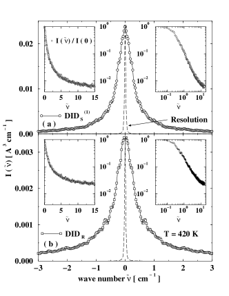
Figure 1: (a) First order DID spectrum calculated considering the carbon atoms (model S) at $T=420$ K together with the resolution curve (see text for details). The insets show the data, renormalized to the peak intensity, in semi-logarithmic (left panel) and logarithmic scale (right panel), in order to stress the power law behavior of the tail. (b) DID spectrum calculated considering the phenyl rings centers of mass (model R).

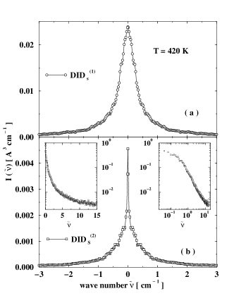
Figure 2: (a) As in Fig. 1(a). (b) Second order DID calculated for model S.

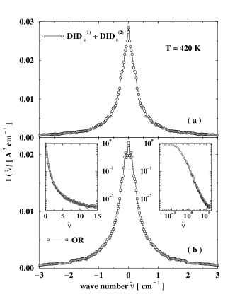
Figure 3: (a) Sum of first and second order DID terms for the $S$ model. (b) Orientational contribution to the spectrum.

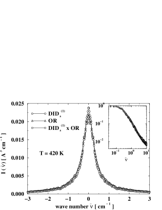
Figure 4: Contributions to the total spectrum for the S model: first order DID (circles), orientational contribution (triangles), and cross-correlation (squares) calculated at $T=420$ K; the inset shows the same data, renormalized to the respective peak intensities, in a double-logarithmic scale.

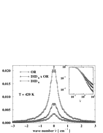
Figure 5: Contributions to the total spectrum for the $R$ model: first order DID (circles), orientational contribution (triangles) and cross-correlation (squares) calculated at $T=420$ K; the inset shows the same data, renormalized to the respective peak intensities, in a double-logarithmic scale.

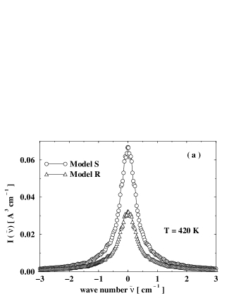
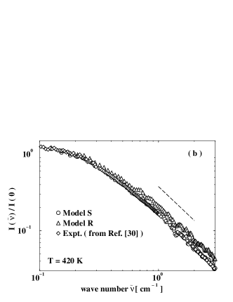
Figure 6: (a) Total spectra for the S (circles) and R (triangles) models. (b) Total spectra for the S (circles) and R (triangles) models together with the experimental results ($V_{H}$ spectra from Ref. Angelini99 ) at $T=444$ K (diamonds) in a double logarithmic scale. A power law of exponent $\lambda=-1.5$ (dashed line) is also plotted as a guide to the eye.

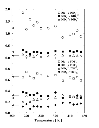
Figure 7: (a) Ratios between the first order DID contribution to the $S$ model and the other terms as a function of temperature: Orientational (circles), DID calculated for model R (full squares) and second order DID calculated for model S (triangles). The arrows indicate the mean values that are respectively $1.22$, $0.25$, and $0.09$. (b) Relative intensity of the different contributions with respect to the total intensity calculated with both models. The arrows indicate the mean values of respectively $0.66$, $0.32$ $0.27$, and $0.14$.

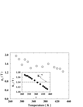
Figure 8: Static angular pair correlation factor $g_{2}(T)$ (Eq. (8)) as a function of temperature. In the inset, $K_{2}(T)$ (Eq. (10)) is shown as a function of temperature.

IV COMPUTATIONAL DETAILS

We study a system composed by $108$ OTP molecules ($324$ rings, $1944$ LJ interaction sites) enclosed in a cubic box with periodic boundary condition. The MD runs are performed in the microcanonical (NVE) ensemble. To integrate the equations of motion we treats each ring as a separate rigid body, identified by the position of its center of mass ${\bm{R}}_{i}$ and by its orientation, expressed in terms of quaternions ${\bm{q}}_{i}$ allen . The standard Verlet leap-frog algorithm allen has been implemented to integrate the translational motion while, for the most difficult orientational part, a refined algorithm has been used ruosam . The integration time-step is $\Delta t$=2 fs, which gives rise to an overall energy conservation better than 0.01 % of the kinetic energy.

We consider two series of runs. For temperature $T=420$ K, to be compared with the experimental results, we perform one run $24$ ns long with a saving time of $1$ ps; using windows $800$ ps wide we achieve a resolution of 0.04 cm^-1. For the temperatures $T=$ 280, 290, 300, 310, 320, 330, 350, 370, 390, 410 and 430 K we run for $640$ ps with a saving time of $0.04$ ps; using windows of $320$ ps we reach a resolution of 0.1 cm^-1.

In the R scheme, the components of the polarizability tensor (in the molecular fixed frame) are $\alpha_{\parallel}=12.31$ $\AA^{3}$, $\alpha_{\perp}=6.35$ $\AA^{3}$, $\alpha=1/3(\alpha_{\perp}+2\alpha_{\parallel})=10.32$ $\AA^{3}$, $\gamma=\alpha_{\perp}-\alpha_{\parallel}=-5.96$ $\AA^{3}$, where $\perp$ stands for orthogonal to the phenyl ring’s plane, i.e. parallel to the symmetry axis. These values are taken from the polarizability tensor of the benzene hirsch . For the S scheme, to each site have been attributed the previous values divided by $6$ and the same orientation.

V RESULTS AND DISCUSSION

In Fig. 1 the DID spectrum at first order is reported in the liquid phase at $420$ K for both S (Fig. 1(a)) and R (Fig. 1(b)) schemes. The dashed lines refer to the obtained resolution, which depends on the time length of the MD run. In the insets the same data, rescaled to the peak intensity, are shown in semi-logarithmic (left) and logarithmic (right) scale in order to emphasize the power law behavior of the tails.

As expected, the overall intensity in the S scheme is much higher than the one in the R scheme. On the contrary, the shape is very similar, although the relative intensity of the spectral wings (at 10 $cm^{-1}$) with respect to the peak intensity is about three times higher in the R scheme. As a consequence the absolute wing intensities are comparable. On the overall, the shape is similar to the induced contribution from heavy noble gases, i.e., an exponential decay of the form $\exp(-\omega/\omega_{o})$ with $\omega_{o}$ of the order of 2 $cm^{-1}$.

Only for the S scheme the second order DID is of some importance, so in Fig. 2 the corresponding spectrum (Fig 2(b)) is compared with the first order DID (Fig 2(a)). At all frequencies the second order contribution is a relatively small fraction of the first one; above 0.25 cm^-1 it is less than about 10$\%$, so the DID’s at higher order can be safely neglected.

The sum of the first and second order DID, and the orientational spectra in the S scheme are compared in Fig. 3(a) and (b) respectively. As we can see, the relative shapes and intensities in this case are quite similar (apart from the shape of the peak at frequency comparable to the spectral resolution, where the simulation statistical errors are large and prevent any reliable comparison). We want to stress that no time scale separation is detectable between translational and orientational dynamics. This is reflected also in the shape and high intensity of the cross contribution; at this temperature, indeed, the spectra of orientational, DID and cross contributions practically superimpose each other, as shown in Fig. 4.

In the case of the R scheme, the situation is quite different. Beyond the smaller relative importance of the DID and cross terms, at high frequency (above 5 cm^-1) the spectrum is dominated by the DID contributions, even if at 10 cm^-1 the ratio of DID, cross and orientational contributions is not so high, being $4:2:1$ (see Fig. 5).

Again, even in R scheme our simulations are in poor agreement with the assumptions made by Patkowski et al. Pecora97 about the spectral separation between orientational and DID contributions. Indeed, it is evident from Fig. 5 that no time scale separation can be effective and the cross term cannot be neglected.

The resulting — total — simulated DLS spectra for the two schemes are reported in Fig. 6(a). In Fig. 6(b) we show, in double logarithmic scale, a comparison of the two line shapes with the experimental spectrum at $444$ K Angelini99 . The agreement among the sets of data is quite good, considering the approximations we have made in the dynamical and polarizability model. This shape comparison gives some preference to the S scheme, but it is hard to really discriminate between these two limiting polarizability models on this basis. R and S DLS spectra differ essentially in intensity rather then in shape, and some help would come from an absolute intensity comparison; unfortunately, the OTP experimental absolute intensity has not been calculated so far. Anyway, the large uncertainties usually present in both experimental and simulated determinations of DLS absolute spectral intensities, could not allow this kind of comparison.

In Fig. 7 we plot the temperature dependence of the relative integrated intensities of the various spectral contributions. We see that the relative intensities do not show any significant trend with temperature, apart from a tendency of the orientational part to increase at the lowest investigated temperatures. The increase has to be attributed to a change in the relative orientation of the rings, i.e., to an increasing of $g_{2}$. This is clearly seen in Fig. 8 where $g_{2}$ (main panel) and $K_{2}$ Inset) are plotted as a function of temperature. It is interesting to note that also $K_{2}$ increases on decreasing temperature, being less than the reference value $K_{2}^{eq}\simeq$ 1.14 at high temperatures and more than that value at low temperatures. On the basis of the value of the angles between the symmetric top axis of the rings, $K_{2}$ increases fast if there is a spread of ${\bf n}_{1}\cdot{\bf n}_{2}$ and ${\bf n}_{1}\cdot{\bf n}_{3}$, but decreases with the spread of ${\bf n}_{2}\cdot{\bf n}_{3}$. The distribution of angle cosines is reported in Fig. 6 of Ref. Mossa00 . At high temperatures, the large spread of ${\bf n}_{2}\cdot{\bf n}_{3}$ is, anyway, able to decrease $K_{2}$ under $K_{2}^{eq}$, but at low temperature the situation is reversed by the spread of ${\bf n}_{1}\cdot{\bf n}_{2}$ and ${\bf n}_{1}\cdot{\bf n}_{3}$.

We expect a similar situation to hold for the DLS of a large class of molecular glass forming liquids: the DLS would be a mixture of orientational, DID and cross contributions in the entire low frequency range, with no significant time scale separation. Further, the better agreement with the experimental results of the S scheme in the case of OTP, underlines the importance to take into account the internal degrees of freedom to obtain a realistic description of the DLS of glass forming liquids consisting of large flexible molecules.

VI CONCLUSIONS

In this paper we have studied, by means of molecular dynamics simulations, the orientational and induced contributions to the low frequency depolarized Rayleigh spectra of supercooled ortho-terphenyl. We have used a realistic flexible intramolecular model recently introduced by some of us, taking into account the most important internal degrees of freedom of the OTP molecule. Two polarizability models have been introduced, each of them considering a different scattering unit. In the ring’s model R, we have assigned to each phenyl ring the polarizability of the benzene. In the site’s model S, we have assigned to the sites of each ring the same polarizability divided by six. This procedure has allowed us to study the single contributions to the DLS spectra in both cases. Our main findings are the following: i) Although in the two schemes the intensities of the DID contributions are very different, their overall shape is very similar; ii) The second order DID is at all frequencies already a relatively small fraction of the first order contributions, so that all the higher induced terms can be safely neglected; iii) For the S model first order DID and orientational contributions are very similar in both shape and intensity; iv) In both models the cross correlation between induced and orientational terms cannot be neglected. This fact is in striking contrast with the analysis of the experimental data of Ref. Pecora97 and support the conclusion that: v) No time scale separation is present between DID and orientational contribution. In other words we expect that, similarly to the present case, for a broad class of molecular glass forming liquids the DLS spectra would be a superposition of DID, orientational and mixed contributions, and none of them should be disregarded. Finally: vi) the better agreement of the S scheme calculated spectra with the experimental results underlines the importance of taking into account the molecular internal degrees of freedom in order to obtain a realistic description of complex molecular liquids.

ACKNOWLEDGEMENTS

This work was supported by MURST PRIN 2000.

References

- (1) B. J. Berne and R. Pecora, Dynamic Light Scattering (Wiley, New York, 1976).
- (2) N. J. Tao, G. Li, X. Chen, W. M. Du, and H. Z. Cummins, Phys. Rev. A 44, 6665 (1991).
- (3) G. Li, W. M. Du, X. K. Chen, H. Z. Cummins, and N. J. Tao, Phys.Rev. A 45, 3867 (1992).
- (4) W. M. Du, G. Li, X. Chen, H. Z. Cummins, M. Fuchs, J. Toulouse, and L. A. Knauss, Phys. Rev. E 49, 2192 (1994).
- (5) J. Wuttke, J. Hernandez, G. Li, G. Coddens, H. Z. Cummins, F. Fujara, W. Petry, and H. Sillescu, Phys. Rev. Lett. 72, 3052 (1994).
- (6) A. D. Bykhovskii and R. M. Pick, J. Chem. Phys. 100, 7109 (1994).
- (7) M. J. Lebon, C. Dreyfus, G. Li, A. Aouadi, H. Z. Cummins, and R. M. Pick, Phys. Rev. E 51, 4537 (1995).
- (8) C. Alba-Simionesco and M. Krauzman, J. Chem. Phys. 102, 6574 (1995).
- (9) W. Götze and L. Sjögren, Rep. Prog. Phys. 55, 241 (1992).
- (10) H. Z. Cummins, G. Li, W. Du, R. Pick, C. Dreyfus, Phys. Rev. E 53, 896 (1996).
- (11) A. Patkowski, W. Steffen, H. Nilgens, E. W. Fisher, and R. Pecora, J. Chem. Phys. 106, 8401 (1997).
- (12) S. Mossa, R. Di Leonardo, G. Ruocco, and M. Sampoli, Phys. Rev. E 62, 612 (2000).
- (13) S. Mossa, G. Ruocco, and M. Sampoli, Phys. Rev. E 64, 021511 (2001).
- (14) S. Mossa, G. Monaco, G. Ruocco, M. Sampoli, and F. Sette, J. Chem. Phys. 116, 1077 (2002).
- (15) S. Mossa, G. Monaco, and G. Ruocco, Preprint cond-mat/0104265.
- (16) For a review of induced contribution see G. Birnbaum (editor), Phenomena Induced by Intermolecular Interactions (Plenum, New York, 1985).
- (17) P. D. Dacre, Canad. J. Phys. 59, 1439 (1981); ibid. 60, 963 (1982); Mol. Phys. 36, 541 (1978); ibid. 45, 1 (1982); ibid., 17; ibid. 47, 193 (1982).
- (18) K. L. C. Hunt in G. Birnbaum (editor), Phenomena Induced by IntermolecularInteractions (Plenum, New York 1985), 263.
- (19) F. Barocchi and M. Zoppi, in G. Birnbaum (editor), Phenomena Induced by Intermolecular Interactions (Plenum, New York 1985), 311.
- (20) F. Barocchi, F. Hensel, and M. Sampoli, Chem. Phys. Lett. 232, 445 (1995).
- (21) J. Applequist, J. R. Carl, and K. K. Fung, J. Am. Chem. Soc. 94, 2952 (1972).
- (22) M. L. Olson and K. R. Sundberg, J. Chem. Phys. 69, 5400 (1978).
- (23) B. T. Thole, Chem. Phys. 59, 341 (1981).
- (24) J. Applequist, J. Phys. Chem. 97, 6016 (1993).
- (25) H. Stassen, Th. Dorfmuller, and B. M. Ladanyi, J. Chem. Phys. 100, 6318 (1994).
- (26) A. Ben-Reuven and N. D. Gershon, J. Chem. Phys. 51, 893 (1969).
- (27) M. P. Allen and D. J. Tildesley, Computer Simulation of Liquids(Clarendon Press, Oxford, 1989).
- (28) G. Ruocco and M. Sampoli, Mol. Phys. 82, 875 (1994).
- (29) J. O. Hirschfelder, C. F. Curtiss, and R. B. Bird, Molecular Theory of Gases and Liquids (Wiley, New York, 1967).
- (30) R. Angelini, Thesis, Università di L’Aquila, 1999.