Compression and Diffusion: A Joint Approach to Detect Complexity

Abstract

The adoption of the Kolmogorov-Sinai (KS) entropy is becoming a popular research tool among physicists, especially when applied to a dynamical system fitting the conditions of validity of the Pesin theorem. The study of time series that are a manifestation of system dynamics whose rules are either unknown or too complex for a mathematical treatment, is still a challenge since the KS entropy is not computable, in general, in that case. Here we present a plan of action based on the joint action of two procedures, both related to the KS entropy, but compatible with computer implementation through fast and efficient programs. The former procedure, called Compression Algorithm Sensitive To Regularity (CASToRe), establishes the amount of order by the numerical evaluation of algorithmic compressibility. The latter, called Complex Analysis of Sequences via Scaling AND Randomness Assessment (CASSANDRA), establishes the complexity degree through the numerical evaluation of the strength of an anomalous effect. This is the departure, of the diffusion process generated by the observed fluctuations, from ordinary Brownian motion. The CASSANDRA algorithm shares with CASToRe a connection with the Kolmogorov complexity. This makes both algorithms especially suitable to study the transition from dynamics to thermodynamics, and the case of non-stationary time series as well. The benefit of the joint action of these two methods is proven by the analysis of artificial sequences with the same main properties as the real time series to which the joint use of these two methods will be applied in future research work.

¹ Istituto di Linguistica Computazionale del Consiglio Nazionale delle
Ricerche, Area della Ricerca di Pisa, Via Alfieri 1, San Cataldo, 56010, Ghezzano-Pisa, Italy
²Dipartimento di Matematica Applicata, Università di Pisa, Via Bonanno 26/b, 56127 Pisa, Italy
³ Centro Interdisciplinare per lo Studio dei Sistemi Complessi, Università di Pisa, Via Bonnanno, 25/b 56126 Pisa, Italy
⁴Center for Nonlinear Science, University of North Texas, P.O. Box 311427, Denton, Texas 76203-1427
⁵Dipartimento di Fisica dell’Università di Pisa and INFM Piazza Torricelli 2, 56127 Pisa, Italy
⁶Istituto di Biofisica del Consiglio Nazionale delle Ricerche,
Area della Ricerca di Pisa, Via Alfieri 1, San Cataldo, 56010, Ghezzano-Pisa, Italy
⁷ Center for Nonlinear Science, Texas Woman’s University, P.O. Box 425498, Denton, Texas 76204
⁸ International School for Advanced Studies, Via Beirut 4, 34014 Trieste, Italy

1 Introduction

The KS entropy is a theoretical tool widely used by physicists for an objective assessment of randomness[19, 9]. We consider a sequence of symbols $\omega_{i}$, and we use a moving window of size $l$, with $l$ being an integer number. This means that we can accommodate within this window $l$ symbols of the sequence, in the order they appear, and that moving the window along the sequence we can detect combinations of symbols that we denote by $\omega_{0}\omega_{1}\ldots\omega_{l-1}$. In principle, having available an infinitely long sequence and a computer with enough memory and computer time, for any combination of symbols we can evaluate the corresponding probability $p(\omega_{0},\omega_{1},\ldots\omega_{l-1})$. Consequently, the $l$-th order empirical entropy is

$$H_{l}=-\sum_{\omega_{0}\omega_{1}\ldots\omega_{l-1}}p(\omega_{0},\omega_{1},\ldots\omega_{l-1})\ln(p(\omega_{0},\omega_{1},\ldots\omega_{l-1})).$$ (1)

The KS entropy is defined as

$$h_{KS}=lim_{l\rightarrow\infty}\frac{H_{l}}{l}.$$ (2)

This way of proceeding is of only theoretical interest since the KS computer evaluation can hardly exceed a window length of order $10$ [16]. The reason why the KS is so popular depends on the Pesin theorem [19, 9]. In the specific case where the symbolic sequence is generated by a well defined dynamic law, the Pesin theorem affords a practicable criterion to evaluate the KS entropy. To make an example, let us assume that the dynamic law is expressed by

$$x_{n+1}=\Pi(x_{n}),$$ (3)

in the interval $[0,1]$, where $\Pi$ has a derivative $\Pi^{\prime}$. Using the Pesin theorem[19, 9] we can express $h_{KS}$ under the form

$$h_{KS}=\int_{0}^{1}ln|\Pi^{\prime}(x)|\rho(x)dx,$$ (4)

where $\rho(x)dx$ denotes the invariant measure whose existence is essential for the Pesin theorem to work.

In practice, the statistical analysis of a system of sociological, biological and physiological interest, is done through the study of a time series. This is a seemingly erratic sequence of numbers, whose fluctuations are expected to mirror the complex dynamics of the system under study. In general, we are very far away from the condition of using any dynamic law, not to speak of the one-dimensional picture of Eq. (3). Thus the randomness assessment cannot be done by means of Eq. (4). Furthermore, there is no guarantee that a real time series refers to the stationary condition on which the Pesin theorem rests. This might mean that the invariant distribution does not exist, even if the rules behind the complex system dynamics do not change with time. The lack of an invariant distribution might be the consequence of an even worse condition: this is when these rules do change with time. How to address the statistical analysis of a real process, in these cases?

The main purpose of this paper is to illustrate the main ideas to bypass these limitations. This is done with the joint use of two techniques, both related in a way that will be discussed in this paper, to the KS entropy. Both methods serve the purpose of making the KS entropy computable, in either a direct or indirect way. The first method is a compression algorithm. This method applies directly to the time series under study and evaluates its computable content. The second method, on the contrary, does not refer directly to the data of the time series, but it interprets them as diffusion generating fluctuations, and then evaluates the entropy of the resulting diffusion process, hence the name of Diffusion Entropy (DE) method. An interesting goal of this paper is also to illustrate the connections between these two methods.

The outline of the paper is as follows. In Section II we illustrate the compression algorithm method. In Section III we illustrate the DE method. Section IV is devoted to illustrating the dynamical model that we use to create the artificial sequences. In Section V we show CASSANDRA in action in the case of sequences mimicking non-stationary processes. In Section VI we address the central core of this paper, the joint use of CASSANDRA and CASToRE. Section VII illustrate the two methods in action on time series characterized by a mixture of events and pseudo events. What we mean by events and pseudo events will be explained in detail in Section VII. Here we limit ourselves to saying that by event we mean the occurence of a unpredictable fact, while the concept of pesudoevent implies predictability. In Section VIII, using the logistic map at the chaos threshold, we show that the power law sensitivity to initial condition leads to a form of localization with the DE not exceeding a given upper limit. A balance on the results obtained is made in Section IX.

2 The Computable Information Content method

In the first of the two approaches illustrated in this paper the basic notion is the notion of information. Given a finite string $s$ (namely a finite sequence of symbols taken in a given alphabet), the intuitive meaning of quantity of information $I(s)$ contained in $s$ is the length of the smallest binary message from which we can reconstruct $s$. This concept is expressed by the notion of Algorithmic Information Content ($AIC$). We limit ourselves to illustrating the main idea with arguments, intuitive but as close as possible to the formal definition (for further details, see [11] and related references). We can consider a partial recursive function as a computer $C$ which takes a program $p$ (namely a binary string) as an input, performs some computations and gives a string $s=C(p)$, written in the given alphabet, as an output. The $AIC$ of a string $s$ is defined as the shortest binary program $p$ which gives $s$ as its output, namely

$$I_{AIC}(s,C)=\min\{|p|:C(p)=s\},$$

where $|p|$ means the length of the string $p$. From this point of view, the shortest program $p$ which outputs the string $s$ is a sort of optimal encoding of $s$. The information that is necessary to reconstruct the string is contained in the program. Unfortunately, this coding procedure cannot be performed on a generic string by any algorithm: the Algorithmic Information Content is not computable by any algorithm (see Chaitin theorem in [18]).

Another measure of the information content of a finite string can also be defined by a loss-less data compression algorithm $Z$ satisfying some suitable properties which we shall not specify here. Details are discussed in [11]. We can define the information content of the string $s$ as the length of the compressed string $Z(s),$ namely,

$$I_{Z}\left(s\right)=\left|Z(s)\right|.$$

The advantage of using a compression algorithm lies in the fact that, this way, the information content $I_{Z}\left(s\right)$ turns out to be a computable function. For this reason we shall call it Computable Information Content $(CIC)$. In any case, given any string $s,$ we assume to have defined the quantity $I(s)$ via $AIC$ or via $CIC.$ If $\omega$ is an infinite string, in general, its information is infinite; however it is possible to define another notion: the complexity. The complexity $K(\omega)$ of an infinite string $\omega$ is the average information $I$ contained in a single digit of $\omega$, namely,

$$K(\omega)={\limsup}_{n\rightarrow\infty}\frac{I(\omega^{n})}{n},$$ (5)

where $\omega^{n}$ is the string obtained taking the first $n$ elements of $\omega.$ If we equip the set of all infinite strings $\Omega$ with a probability measure $\mu$, the couple $(\Omega,\mu)$ can be viewed as an information source, provided that $\mu$ is invariant under the natural shift map $\sigma$, which acts on a string $\omega=(\omega_{i})_{i\in\mathbf{N}}$ as follows: $\sigma(\omega)=\tilde{\omega}$ where $\tilde{\omega}_{i}=\omega_{i-1}\ \forall i\in\mathbf{N}$. The entropy $h_{\mu}$ of $(\Omega,\mu)$ can be defined as the expectation value of the complexity:

$$h_{\mu}=\int_{\Omega}K(\omega)\;d\mu\ .$$ (6)

If $I\left(\omega\right)=I_{AIC}\left(\omega\right)$ or $I\left(\omega\right)=I_{Z}\left(\omega\right),$ under suitable assumptions on $Z$ and $\mu,$ $h_{\mu}$ turns out to be equal to the Shannon entropy. Notice that, in this approach, the probabilistic aspect does not appear in the definition of information or complexity, but only in the definition of entropy.

Chaos, unpredictability and instability of the behavior of dynamical systems are strongly related to the notion of information. The KS entropy illustrated in Section I can be interpreted as the average measure of information that is necessary to describe a step of the evolution of a dynamical system. As seen in Section I, the traditional definition of KS entropy is given by the methods of probabilistic information theory: this corresponds to the a version of the Shannon entropy adapted to the world of dynamical systems.

We have seen that the information content of a string can be defined either with probabilistic methods or using the $AIC$ or the $CIC$. Similarly, also the KS entropy of a dynamical system can be defined in different ways. The probabilistic method is the usual one, the $AIC$ method has been introduced by Brudno [15]; the $CIC$ method has been introduced in [22] and [6]. So, in principle, it is possible to define the entropy of a single orbit of a dynamical system (which we shall call, as sometimes it has already been done in the literature, complexity of the orbit). There are different ways to do this (see [15], [23], [26], [13] , [24]). In this paper, we consider a method which can be implemented in numerical simulations. Now we shall describe it briefly.

Using the usual procedure of symbolic dynamics, given a partition $\alpha$ of the phase space of the dynamical system $\left(X,\mu,T\right)$, it is possible to associate a string $\Phi_{\alpha}\left(x\right)$ to the orbit having $x$ as initial condition. If $\alpha=(A_{1},\dots,A_{l}),$ then $\Phi_{\alpha}\left(x\right)=(s_{0},s_{1},\dots,s_{k},\dots)$ if and only if

$$T^{k}x\in A_{s_{k}}\quad\forall\ k\ .$$

If we perform an experiment, the orbit of a dynamical system can be described only with a given degree of accuracy related to the partition of the phase space $X$. A more accurate measurement implies a finer partition of $X.$ The symbolic orbit $\Phi_{\alpha}\left(x\right)$ is a mathematical idealization of these measurements. We can define the complexity $K(x,\alpha)$ of the orbit with initial condition $x$ with respect to the partition $\alpha$ in the following way

$$K(x,\alpha)={\limsup}_{n\rightarrow\infty}\frac{I(x,\alpha,n)}{n},$$

where

$$I(x,\alpha,n):=I(\Phi_{\alpha}\left(x\right)^{n}).$$ (7)

Here $\Phi_{\alpha}\left(x\right)^{n}$ represents the first $n$ digit of the string $\Phi_{\alpha}\left(x\right).$ Letting $\alpha$ vary among all the computable partitions, we set

$$K(x)=\sup_{\alpha}K(x,\alpha)\ .$$

The number $K(x)$ can be considered as the average amount of information necessary to ”describe” the orbit in the unit time when we use a sufficiently accurate measurement device.

The notion of ”computable partition” is based on the idea of computable structure which relates the abstract notion of metric space with computer simulations. The formal definitions of computable partition are given in [25]. We limit ourselves to describing its motivation. Many models of the real world use the notion of real numbers or more in general the notion of complete metric spaces. Even if we consider a very simple complete metric space, as, for example, the interval $\left[0,1\right]$, we note that it contains a continuum of elements. This fact implies that most of these elements (numbers) cannot be described by any finite alphabet. Nevertheless, in general, the mathematics of complete metric spaces is simpler than the ”discrete mathematics” in making models and the relative theorems. On the other hand, the discrete mathematics allows to make computer simulations. A first connection between the two worlds is given by the theory of approximation. But this connection becomes more delicate when we need to simulate more sophisticated objects of continuum mathematics. For example, an open cover or a measurable partition of $\left[0,1\right]$ is very hard to simulate by computer; nevertheless, these notions play a crucial role in the definition of many quantities as, e. g., the KS entropy of a dynamical system or the Brudno complexity of an orbit. For this reason, in the earlier work leading to the foundation of the first method of this paper, the notion of ”computable structure” was introduced. This is a new way to relate the world of continuous models with the world of computer simulations. The intuitive idea of computable partition is the following one:

a partition is computable if it can be recognised

by a computer.

For example, an interval $\left[a,b\right]$ belongs to a computable partition if both $a$ and $b$ are computable real numbers. In particular, a computable partition contains only a enumerable number of elements.

In the above construction, the complexity of each orbit $K(x)$ is defined independently of the choice of an invariant measure. In the compact case, if $\mu$ is an invariant measure on $X$ then $\int_{X}K(x)\;d\mu$ equals the KS entropy. In fact, in [11] it has been proved the following result.
Theorem. If $(X,\mu,T)$ is a dynamical system on a compact space and $\mu$ is ergodic, then for $\mu$-almost each $x\in X$ it holds:

$$K_{Z}(x)=K_{AIC}(x)=h_{\mu}(T)\ \ .$$ (8)

In other words, in an ergodic dynamical system, for almost all points $x\in X,\;$ and for suitable choice of the partition $\alpha,\;I(x,\alpha,n)\sim h_{\mu}n.$ Notice that this result holds for a large class of Information functions $I$ as for example the $AIC$ and the $CIC.$ Thus we have obtained an alternative way to understand the meaning of the KS entropy.

The above construction makes sense also for a non stationary system. Its average over the space $X$ is a generalization of the KS entropy to the non stationary case. Moreover, the asymptotic behavior of $I(x,\alpha,n)$ gives an invariant of the dynamics which is finer than the KS entropy and is particularly relevant when the KS entropy is null.

It is well known that the KS entropy is related to the instability of the orbits. The exact relations between the KS entropy and the instability of the system is given by the Pesin theorem. We shall recall this theorem in the one-dimensional case. Suppose that the average rate of separation of nearby starting orbits is exponential, namely,

$$\Delta x(n)\simeq\Delta x(0)^{\lambda n}\;\;\;\mathrm{for}\Delta x(0)\ll 1,$$

where $\Delta x(n)$ denotes the distance of these two points at time $n$. The number $\lambda$ is called Lyapunov exponent; if $\lambda>0$ the system is unstable and $\lambda$ can be considered a measure of its instability (or sensitivity to the initial conditions). The Pesin theorem implies that, under some regularity assumptions, $\lambda$ equals the KS entropy.

There are chaotic dynamical systems whose entropy is null: usually they are called weakly chaotic. Weakly chaotic dynamics appear in the field of self-organizing systems, anomalous diffusion, long- range interactions and many others. In such dynamical systems the amount of information necessary to describe $n$ steps of an orbit is less than linear in $n$, then the KS entropy is not sensitive enough to distinguish the various kinds of weakly chaotic dynamics. Nevertheless, using the ideas we illustrate in this section, the relation between initial data sensitivity and information content of the orbits can be extended to these cases.

To give an example of such a generalization, let us consider a dynamical system $([0,1],T)$ where the transition map $T$ is constructive, and the function $I(x,\alpha,n)$ is defined using the $AIC$ in a slightly different way than before (use open coverings instead of partitions, see [24]). If the speed of separation of nearby starting orbits goes like $\Delta x(n)\simeq\Delta x(0)f(x,n)$, then for almost all the points $x\in[0,1]$ we have

$$I(x,\alpha,n)\sim\log(f(x,n)).$$ (9)

In particular, if we have power law sensitivity ($\Delta x(n)\simeq\Delta x(0)n^{p}$), the information content of the orbit is

$$I(x,\alpha,n)\sim p\log(n)\ .$$ (10)

If we have a stretched exponential sensitivity ( $\Delta x(n)\simeq\Delta x(0)2^{\lambda n^{p}}$, $p<1$) the information content of the orbits will increase with the power law:

$$I(x,\alpha,n)\sim n^{p}.$$ (11)

Since we have shown that the analysis of $I(x,\alpha,n)$ gives useful information on the underlying dynamics and since $I(x,\alpha,n)$ can be defined through the $CIC$ methodology, it turns out that it can be used to analyze experimental data using a compression algorithm which is efficient enough and which is fast enough to analyze long strings of data. We have implemented a particular compression algorithm we called CASToRe: Compression Algorithm Sensitive To Regularity ([6]).

CASToRe is an encoding algorithm based on an adaptive dictionary and it is a modification of the LZ78 algorithm. Roughly speaking, this means that it translates an input stream of symbols (the file we want to compress) into an output stream of numbers, and that it is possible to reconstruct the input stream knowing the correspondence between output and input symbols. This unique correspondence between sequences of symbols (words) and numbers is called the dictionary. The dictionary is adaptive because it depends on the file under compression, in this case the dictionary is created while the symbols are translated.

At the beginning of encoding procedure, the dictionary is empty. In order to explain the principle of encoding, let us consider a point within the encoding process, when the dictionary already contains some words. The algorithm starts analyzing the stream, looking for the longest word W in the dictionary matching the stream. Then it looks for the longest word Y in the dictionary where W + Y matches the stream. The new word to add to the dictionary would be W + Y. More details on its internal running are described in the Appendix of [11]. In the following, the numerical results addressed to the CIC method have been performed using the algorithm CASToRe.

3 The DE method

Let us now illustrate the second of the two methods of analysis of this paper. This method rests on DE used for the first time in Ref. [35]. This method turned out to be a very efficient and reliable way to determine scaling [28]. Here, after a short review of the DE method, we argue that the DE is not only a method of scaling detection and that with the use of two windows it can be expressed in a form that turns out to be very efficient to study the case of rules changing with time.

The first step of the DE method is the same as that of the pioneering work of Refs.[33, 34]. This means that the experimental sequence is converted into a kind of Brownian-like trajectory. The second step aims at deriving many distinct diffusion trajectories with the technique of moving windows of size $l$. The reader should not confuse the mobile window of size $l$ with the mobile window of size $L$ that will be used later on in this paper to detect non-stationary properties. For this reason we shall refer to the mobile windows of size $L$ as large windows, even if the size of $L$ is relatively small, whereas the mobile windows of size $l$ will be called small windows. The large mobile window has to be interpreted as a sequence on its own, with local statistical properties to reveal, and will be analyzed by means of small windows of size $l$, with $l<L$. The success of the method depends on the fact that the DE makes a wise use of the statistical information available. In fact, the small windows overlap and are obtained by locating their left border on the first site of the sequence, on the second second site, and so on. The adoption of overlapping mobile windows is dictated by the wish of establishing a connection with the KS [9, 19] method, and it has the effect of creating many more trajectories than the Detrended Fluctuation Analysis (DFA)[33, 34].

In conclusion, we create a conveniently large number of trajectories by gradually moving the small window from the first position, with the left border of the small window coinciding with the first size of the sequence, to the last position, with the right border of the small window coinciding with the last site of the sequence:

$$x_{k}(l)=\Sigma_{s=k}^{k+l-1}\xi(s)\ ,\ \ \ 0<k<N-l+1\ .$$

After this stage, we utilize the resulting trajectories, all of them with the initial position located at $x=0$, to produce a probability distribution at “time” $l$:

$$p(x,l)\ =\ \Sigma_{k=0}^{N-l+1}\delta_{x_{k}(l),x},$$

where $\delta_{i,j}$ denotes the delta of Kronecker.

According to a tenet of the Science of Complexity [8, 31], complexity is related to the concept of diffusion scaling. Diffusion scaling is defined by

$$p(x,l)=\frac{1}{l^{\delta}}F(\frac{x}{l^{\delta}}).$$ (12)

Complex systems are expected to generate a departure from the condition of ordinary diffusion, where $\delta=0.5$ and $F(y)$ is a Gaussian function of $y$. For this reason one of the goals of the statistical analysis of time series [33, 34] is the determination of $\delta$. The methods currently adopted measure the second moment of the diffusion process, $<x^{2}>\propto t^{2H}$. However, the validity of this way to detect scaling is questionable since the parameter $H$, usually called Hurst coefficient [33, 34], is known to coincide with $\delta$ only in the case of fractional Brownian motion [31]. It is known that not always the scaling of the second moment is a fair representation of the property of Eq. (12). For instance, the work on dynamic approach to Lévy processes [3] shows that that the second moment yields a scaling different from the scaling corresponding to the definition of Eq. (12). The DE method, on the contrary, if the condition of Eq. (12) is fulfilled, yields the correct value for the scaling parameter $\delta$. Let us see why. The Shannon entropy of the diffusion process reads

$$S(l)=-\int_{\infty}^{+\infty}p(x,l)\ln p(x,l)dx.$$ (13)

Let us plug Eq. (12) into Eq. (13). After some trivial change of integration variable we get

$$S(l)=A+\delta\ln(l),$$ (14)

where $A$ is a constant, whose explicit form is of no interest for the current discussion. From Eq. (14) we derive a natural way to measure the scaling $\delta$ without recourse to any form of detrending.

However, it is worth pointing out that the $DE$ is not only a way to detect scaling. It is much more than that, and one of the main purposes of this paper is to illustrate these additional properties with the help of the perspective of the computable information content, illustrated in Section II. To be more specific, we shall study the DE in action in the case of diffusion processes generated by a dynamic process with either the stretched exponential sensitivity of Eq. (11) or the power law sensitivity of Eq. (10). We shall see that in those specific cases the DE method of analysis allows us to shed light into the fascinating process of transition from dynamics to thermodynamics that is made to become visible when those anomalous conditions apply. We shall see also that the time size of the process of transition from dynamics to thermodynamics is enhanced by the superposition of a random and deterministic process. We shal illustrate this property with an apparently trivial dynamical model. This is the case where the time series under study consists of the sum of a regular motion (a harmonic oscillation) and a completely random process. We shall discuss also the case where the harmonic oscillation is replaced by a quasi-periodic process yielding the power law sensitivity of Eq. (10).

In this paper we shall be dealing with two different forms of non-stationarity. The former has to do with fixed dynamic rules, which are, however, incompatible with the existence of an invariant distribution. An example of this kind is given by the Manneville map with $z>2$, and with the dynamic model of Section IV. We recall that a symbolic sequence $\{\sigma_{i}\}$ is stationary if the frequency of each symbol tends to a limit which is different from zero. If we associate a symbolic sequence to an autonomous dynamical system, that sequence may also tend to a vanishing value, thereby implying non-stationarity, in the first sense. The second type of non-stationarity refers to the case when the dynamic rules change upon time change. This has to do with a case that is frequently met, when studying time series (see, for instance, Ref.[35]). In this specific case, we are led to select a portion of the time series, located, for instance, at two distinct specific times. The purpose of the statistical analysis should be to assess if the statistical properties, and consequently the rules responsible for these statistical properties, at these two distinct times are different or not. Since the statistical properties might be time dependent, the portion of sequence to examine cannot be too large. On the other hand, if the size of that portion is relatively small, there is no time for the process to reach the scaling regime. It is precisely with this picture in mind that the authors of Ref. [2] designed a special version of the DE method that they called Complex Analysis of Sequences via Scaling AND Randomness Assessment (CASSANDRA)[2]. Actually, the connection with the non-stationary aspects of the time series under study does not emerge from the literal meaning of the acronym, but rather from the suggestion of the Cassandra myth. This means indeed that the algorithm with the same name as the daughter of Priam and Ecuba is expected to be useful to make prediction on the basis of the assessment of how rules change upon function of time. The idea is that catastrophic events might be preceded by a preliminary slow process with the rules slightly changing in time. It is this slight change of rules that CASSANDRA should detect for prediction purposes.

4 Dynamical Model for Intermittence

Let us consider a simple dynamical model generating events. By event we mean something completely unpredictable. The example here under discussion will clarify what we really mean. Let us consider the equation of motion

$$\dot{x}=\lambda\ x^{z}\ ,\ z>1,$$ (15)

where the variable $x$ moves within the interval $I\equiv[0,1]$. The particle with this coordinate moves from the left to the right. When this particle reaches the right border of the interval $I$ is injected back to a new initial condition within the interval $I$, selected by means of a random number generator. This is an event. Let us imagine that the exit times are recorded. Let us assume that the series under examination is $\{t_{i}\}$, the set of these exit times. Since these exit times are determined by randomly chosen initial conditions, which are not recorded, they can be considered as being manifestations of events. In Section 6 we shall study the case when the set $\{t_{i}\}$ is a mixture of events and pseudo events, and this will serve the purpose of illustrating in a deeper way our philosophical perspective. For the time being, let us limit ourselves to studying a sequence of events. Let us change the sequence $\{t_{i}\}$ into the new sequence $\{\tau_{i}\}$, where

$$\tau_{i}\equiv t_{i+1}-t_{i}.$$ (16)

With very simple arguments similar to those used in [5], and in the earlier work of Ref. [27] as well, we can prove that the probability distribution of these times is given by

$$\psi(\tau)=(\mu-1)\frac{T^{\mu-1}}{(T+\tau)^{\mu}},$$ (17)

with $\mu=z/(z-1)$ and $T=\frac{(\mu-1)}{\lambda}$.

In the special case where $2<\mu$ the mean waiting time is given by

$$<\tau>=\frac{T}{(\mu-2)}.$$ (18)

Using the arguments of Ref. [4] it can be shown that this dynamic model for $\mu>3$ generates ordinary Gaussian diffusion, while for $\mu<3$ (with $\mu>2$ still valid) yields Lévy statistics. From the entropic point of view, however, we do not observe any abrupt change when $\mu$ crosses the border between the Lévy and the Gauss basin of attraction. This corresponds to the general prescriptions of Section II, and it is also supported by intuitive arguments as follows. We assume that the drawing of a random number implies an entropy increase equal to $H_{E}$. It is evident that the rate of entropy increase per unit of time is $H_{E}/{\tau}$, as it can be easily realized by noticing that at a given time $t$ (very large), the number of random drawings is equal to $t/<\tau>$. We note that this heuristic form of entropy must not be confused with the KS entropy. For this reason we use the subscript $E$ standing for external. This means that randomness has an external origin, being dependent on the random drawing of initial condition. The available random number generators are not really random. However, here for simplicity we adopt an idealization where the choice of initial condition is really a random process, this being external to the dynamics illustrated by Eq. (15). We see that this form of entropy, as the KS entropy illustrated in Section II, does not result in any abrupt change when $\mu$ crosses the border between Gauss and Lévy statistics.

The compression algorithm illustrated in Section II, as we have seen, serves the purpose of making the KS entropy computable. Therefore, it is convenient to derive an analytical expression for the KS entropy. This can be done with heuristic arguments inspired to the method proposed by Dorfmann[19]. We create a Manneville-like map with a laminar region and a chaotic region. The key ingredient of this map is given by the parameter $\lambda$, which is assumed to fulfill the condition

$$\lambda<<1.$$ (19)

This means that the integration step, equal to $1$, can be regarded as infinitesimally small. This has important consequences. The original Manneville map[32] reads

$$x_{n+1}=x_{n}+x_{n}^{z},(mod.1),z\leq 1.$$ (20)

The region belonging to the interval $I=[0,d]$, with $d$ defined by $d+d^{z}=1$, is called laminar region and is usually studied by adopting a continuum time approximation. The Manneville map at $z=1$ becomes identical to the Bernoulli shift map, and so to a coin tossing process [9]. The use Eq.(15) with the condition (19) makes it possible for us to reach the limiting condition $z=1$ without ever leaving the continuous time approximation on which Eq.(15) rests. Using this model, the interval $I=[0,1]$ is divided two into portions, the first ranging from $x=0$ to $x=\epsilon$ (laminar region) and the second from $x=\epsilon$ to $x=1$ (chaotic region). The parameter $\epsilon$ is defined by the following condition

$$(1-\epsilon)+\lambda(1-\epsilon)^{z}=1.$$ (21)

The adoption of condition (19) makes the value of $\epsilon$ become very close to that of $\lambda$. The chaotic region is defined by the Bernoulli-like form

$$x_{n+1}=\frac{x_{n}+\epsilon-1}{\epsilon}.$$ (22)

In the limiting case of extremely small $\lambda$’s the size of chaotic region tends to zero, but its contribution to the Lyapunov coefficient cannot be neglected, since it is much larger than the Lyapunov coefficients of the laminar region. The invariant distribution $p(x)$ is shown to be $p(x)=1/x^{1/(\mu-1)}$. Thus, a good approximation to the prescription of the Pesin theorem [19, 9] is given by

$$h_{KS}=\frac{\mu-2}{\mu-1}\left[\int_{0}^{1}\frac{1}{x^{\frac{1}{(\mu-1)}}}\ln(1+\frac{\mu}{T}x^{\frac{1}{\mu-1}})dx+\lambda\ln(\frac{1}{\lambda})\right].$$ (23)

In the case where the parameter $T$ is very large, we can take into account only the first term of the Taylor expansion of the logarithm. The new expression, written as a function of $z$, reads

$$h_{KS}=(2-z)\lambda[z+\ln(1/\lambda)].$$ (24)

We see that when the mean waiting time becomes equal to infinity (at $z=2$, or $\mu=2$) the KS entropy vanishes, a property shared by both KS entropy and external entropy. When we explore $z>2$ (or $\mu<2$) we enter a regime, characterized by very interesting properties. The adoption of the same heuristic arguments as those yielding the KS expression of Eq. (23) makes it possible to prove [30] that the external entropy increase as $t^{\mu-2}$. The information content approach of Section II yields equivalent results. When $1<z<2$, the information content of a trajectory with starting point $x$ and for $n$ steps is

$$I_{AIC}(x,\alpha,n)\sim K\ n\ ,$$ (25)

where the factor $K$ can be considered a numerical estimation of the KS entropy of the system $h_{KS}(T)$. The table shows some numerical results for this case.

z value	$\lambda$ value	KS entropy	Complexity K
1.8	0.1	0.082	0.079
1.5	0.04	0.0943	0.0936
1.2	0.025	0.0977	0.980
1.1	0.022	0.0980	0.993

When $z>2$ the Manneville map is weakly chaotic and non stationary. It can be proved [26], [13], [24] that for almost each $x$ (with respect to the Lebesgue measure)

$$I_{AIC}(x,\alpha,n)\sim n^{\frac{1}{z-1}}\ .$$ (26)

Some numerical results about the exponent are the following:

z	CIC	theoretical value
2.8	0.573	0.555
3	0.533	0.5
3.5	0.468	0.4

5 The Balance between Randomness and Order Changing with Time

We address the problem of detecting non-stationary effects in time series (in particular fractal time series) by means of the DE method. This means that the experimental sequence under study, of size $N$, is explored with a window of size $L<<N$. The artificial sequence under study is described by

$$\xi_{b}(t)=\kappa\xi(t)+Acos(\omega t).$$ (27)

The second term on the right hand side of this equation is a deterministic contribution that might mimic, for instance, the season periodicity of Ref. [35]. The first term on the right hand side is a fluctuation with no correlation that can be correlated, or not, to the harmonic bias.

Fig. 1 refers to the case when the random fluctuation has no correlation with the harmonic bias. It is convenient to illustrate what happens when $\kappa=0$. This is the case where the signal is totally deterministic, being reduced to $\xi_{b}(t)=Acos(\omega t)$. It would be nice if the entropy in this case did not increase upon increasing $l$. However, we must notice that the method of mobile windows implies that many trajectories are selected, the difference among them being a difference on initial conditions. Entropy initially increases. This is due to the fact that the statistical average on the initial conditions is perceived as a source of uncertainty. However, after a time of the order of the period of the deterministic process, a regression to the condition of vanishing entropy occurs, and it repeats at multiples of the period of the deterministic process. Another very remarkable fact is that the maximum entropy value is constant, thereby signaling correctly that we are in the presence of a periodic process: the initial entropy increase, caused by the uncertainty on initial conditions, cannot keep going forever, and it is balanced by the recurrences.

Let us now consider the effect of a non vanishing $\kappa$. We see that the presence of an even very weak random component makes an abrupt transition to occur from the condition where the DE is bounded from above, to a new condition where the recurrences are limited from below by an entropy increase proportional to $0.5\ln l$. In the asymptotic time regime the DE method yields, as required, the proper scaling $\delta=0.5$. However, we notice that it might be of some interest for a method of statistical analysis to give information on the extended regime of transition to the final thermodynamic condition. We notice that if the DE method is interpreted as a method of scaling detection, it might also give the impression that a scaling faster than the ballistic $\delta$ is possible. This would be misleading. However, this aspect of the DE method, if appropriately used, can become an efficient method to monitor the non-stationary nature of the sequence under study, as we shall see with other examples in this section.

Figure 1: The DE $S_{d}(l)$ as a function of time $l$ for different sequences of the type of Eq. (12).

In the special case where the fluctuation $\xi(t)$ is correlated to the bias, the numerical results illustrated in Fig. 2 show that the time evolution of the DE is qualitatively similar to that of Fig. 1. The correlation between the first and the second term on the right hand side of Eq. (27) is established by assuming

$$\xi(t)=\xi_{0}(t)cos(\omega t),$$ (28)

where $\xi_{0}(t)$ is the genuine independent fluctuation, without memory, whose intensity is modulated to establish a correlation with the second term. It is of some interest to mention what happens when $A=0,\kappa=1$, and consequently $\xi_{b}(t)$ coincides with $\xi(t)$ of Eq. (28). In this case we get the straight (solid) line of Fig. 2. This means that the adoption of the assumption that the process is stationary yields a result that is independent of the modulation.

Figure 2: The DE $S_{d}(l)$ as a function of time $l$ for different sequences of the type of Eq. (27) with the prescription of Eq. (28) for the random component.

We use this interesting case to illustrate the extension of the DE method. We note that the name CASSANDRA refers to this extension of the DE method [2]. As earlier mentioned, this extension is based on the use of two mobile windows, one of length $L$ and the traditional one of length $l\ll L$. This means that a large window of size $L$, with $L\ll T=2\pi/\omega$, is located in a given position $i$ of the sequence under study, with $i\leq N-L$, and the portion of the sequence contained within the window is thought of as being the sequence under study. We record the resulting $\delta$ (obtained with a linear regression method) and then we plot it as a function of the position $i$. In Fig. 3 we show that this way of proceeding has the nice effect of making the periodic nature of the process show up, in a condition where the adoption of small windows running over the whole sequence would produce the impression of the existence of a scaling regime.

Figure 3: The method of the two mobile windows applied to a sequence given by Eq. (27.) with $A=0$ and $\xi(t)$ given by Eq. (28). The dashed line represents the amplitude of the harmonic component (not in scale) as a function of the position $i$ of the left border of the large moving window. We selected $L=512$

Let us now improve the method to face non-stationary condition even further. As we have seen, the presence of time dependent condition tends to postpone or to cancel the attainment of a scaling condition. Therefore, let us renounce using Eq. (13) and let us proceed as follows. For any large mobile window of size $L$ let us call $l_{max}$ the maximum size of the small windows. Let us call $n$ the position of the left border of the large window, and and let us evaluate the following property

$$I(n)\equiv\sum_{l=2}^{l_{max}}\frac{S_{d}(l)-[S_{d}(1)+0.5\ln l]}{l}.$$ (29)

The quantity $I(n)$ detects the deviation from the slope that the DE would have in the random case. Since in the regime of transition the entropy increase can be much slower than in the corresponding random case, the quantity $I(n)$ can also bear negative values. This indicator affords a satisfactory way to detect local properties. As an example, Fig. 4 shows a case based on the DNA model of Ref. [1] called Copying Mistake Map (CMM). This is a sequence of symbols $0$ and $1$ obtained from the joint action of two independent sequences, one equivalent to tossing a coin and the other equivalent to establishing randomly a sequence of patches whose length is distributed as an inverse power law with index $\mu$ fitting the condition $2<\mu<3$. The probability of using the former sequence is $1-\epsilon$ and that of using the latter is $\epsilon$. We choose a time dependent value of $\epsilon$:

$$\epsilon=\epsilon_{0}[1-cos(\omega t)].$$ (30)

The adoption of the DE method in the original version [35], namely with only small windows running over the whole sequence of data, would not reveal this periodicity. In Fig. 4 we show that, on the contrary, CASSANDRA, namely the DE method with two kinds of moving windows, makes it possible for us to distinctly perceive a fluctuation around the Brownian scaling, from regions with a scaling faster to regions with a scaling slower than the ordinary scaling $\delta=1/2$. Of course, these scaling fluctuations do not refer to a genuine scaling changing with time, but rather to a processes of transition from dynamics to thermodynamics with a changing rate. From Fig. 4 we see that, although partially random, this changing rate satisfactorily corresponds to the periodicity of Eq. (30).

Figure 4: The method of the two moving windows with $l_{max}=30$ applied to the analysis of an artificial CMM sequence with periodic parameter $\epsilon$. The period of the variation of $\epsilon$ is $5000$ bps and the analysis is carried out with moving windows of size $2000$ bps. Inset: Fourier spectral analysis of $I(n)$.

This paper, as earlier stated, is devoted to illustrating the benefits stemming from the joint use of CASSANDRA and CASToRE by means of artificial sequences. However, before addressing the important issue of the connection between CASToRE and CASSANDRA, whose joint action on real sequences will be illustrated in future work, we want to show CASSANDRA at work on real sequences. Therefore, let us address the problem of the search of hidden periodicities in DNA sequences. Fig. 5 shows a distinct periodic behavior for the human T-cell receptor alpha/delta locus. A period of about 990 base pairs is very clear in the first part of the sequence (promoter region), while several periodicities of the order of $1000$ base pairs are distributed along the whole sequence. These periodicities, probably due to DNA-protein interactions in active eukaryotic genes, are expected by biologists, but the current technology is not yet adequate to deal with this issue, either from the experimental or from the computational point of view: such a behavior cannot be analyzed by means of crystallographic or structural NMR methods, nor would the current (or of the near future) computing facilities allow molecular dynamics studies of systems of the order of $10^{6}$ atoms or more. In conclusion, CASSANDRA (and to the close connection between the two methods, CASToRE as well) can be really adopted with success to analyze real sequences.

Figure 5: The method of two mobile windows applied to the analysis of the human DNA sequence. The method of two mobile windows ($l_{max}=20$ $L=512$) detects a periodicity of 990 bps. Inset: Fourier spectral analysis of $I(n)$.

6 The joint use of CASSANDRA and CASToRE

We now address the issue that is the central core of this paper: the joint use of CASSANDRA and CASToRE. We compare the former to the latter method in a case similar to that of Eq. (27), namely, the case when we have a periodic signal plus noise. We have seen CASSANDRA in action with real number signals. In order to use CASToRe it is necessary to define a symbolic sequence, for instances, $1$’s and $0$’s. As a consequence of the theoretical arguments of Section II, concerning periodic or quasiperiodic signals, CASToRe is expected to yield a logarithmic increase of the CIC. We have seen in Fig. 1 that CASSANDRA in this case yields for $S(t)$ saturation with periodical recurrences. In the case where only randomness is present, the dynamic model of Section V with $\mu>2$, we have seen that $S(t)$ yields the linear increase with respect to the logarithm of time, $S(t)=S(0)+\delta\log(t)$. In this case, we know from Section II that the CIC increases linearly in time. We aim now at exploring these predictions with a close comparison between CASToRE and CASSANDRA.

Let us explain how to generate the first of the two sequences $\{\xi_{n}\}$ that will be used to show both CASToRE and CASSANDRA in action. First we generate the sequence $\{\zeta_{n}\}$ as a periodic sequence repeating a random pattern of 1’s and 0’s of length 100 for 50 times. Then, we build up the first sequence $\{\xi_{n}\}$ following again the prescription of the CMM of ref [1], earlier used in this section. The periodic modulation of Eq. (30) will be used to build up the second sequence. Thus, we define the first sequence as:

$$\xi_{n}=\left\{\begin{array}[]{cccc}\mbox{random}(0,1)&\mbox{with prob.}&\epsilon&\\ \zeta_{n}&\mbox{with prob.}&1-\epsilon,&\\ \end{array}\right.$$ (31)

where the first line stands for a random extraction of either the symbol $1$ or the symbol $0$, by means of a fair coin tossing. In Figs. 6 we illustrate the result of the comparison between the results of CASSANDRA and those of CASToRE, with the left and right columns being devoted to CASSANDRA and CASToRE, respectively. In the first line we illustrate the case when no randomness is present. $S_{d}(t)$ increases for $t<100$, since there is no correlation for time distances smaller than the period $100$. Then it regresses back to $0$, after which it increases and decreases again with periodic recurrences. This behavior is very close to that of Fig. 1. On the other hand, as far as CASToRE is concerned, as explained in Section II, it takes some time for CIC to recognize the sequence periodicity. This means that CASToRE has to store a given number of periods before yielding the logarithmic increase in time dicated by the periodic character of the sequence under study. This expectation is fully confirmed by the top figure of the right column. The lines from the second to the fifth of Fig. 6 illustrate the case when randomness, of increasing intensity, $\epsilon$, is superimposed to the sequence. We make $\epsilon$ vary from $10^{-6}$ to $0.1$. We see that both CASSANDRA and CASToRe have a similar sensitivity to the the amount of randomness. The second line, first column, of Fig. 6 shows that even an infinitesimal value of $\epsilon$ prevents $S(t)$ from regressing to zero. The same second line, second column, shows that the CIC value does not follow anymore a simple logarithmic increase. As $\epsilon$ increases both CASSANDRA and CASToRe make a transition towards the respective behavior that they are expected to show in the case of totally random signals, namely, linear increase with respect to $logt$, the former, and with respect to $t$, the latter.

We now compare CASToRE to CASSANDRA in a case similar to that of Eq. 30. We create a very long sequence with all the sites filled with $0$’s. Then with the probability $\epsilon$ we assign to any site either the symbol $0$, the symbol already there, or the symbol $1$ by tossing a coin. With the probability $1-\epsilon$ we leave the site with the original symbol $0$. In comclusion, we realize the sequence

$$\xi_{n}=\left\{\begin{array}[]{cccc}\mbox{random}(0,1)&\mbox{with prob.}&\epsilon(n)&\\ 0&\mbox{with prob.}&1-\epsilon(n)&.\\ \end{array}\right.$$ (32)

The probability $\epsilon$ is site dependent, and we select the following modulation

$$\epsilon(n)=1-\cos(\Omega n).$$ (33)

At this stage we use the version of CASToRe and CASSANDRA with two moving windows. We remind the reader that, as far as the DE method is concerned, the term CASSANDRA was coined indeed to denote the use of the DE method with the two windows. We have to establish if CASSANDRA and CASToRE perceive correctly the dependence of statistics on site position established by Eq. (33). The results are shown in Fig. 7. Notice that the local AIP with a small windows of length $l=10000$ is effectively able to detect the local amount of noise. As a result we see a local CIC$(n)$ that evolves harmonically in time. The local CASSANDRA indicator defined by Eq. 29 is not sensitive to the global amount of noise: the $S(0)$ component of Eq. 29 would be, but it is subtracted from the indicator $I(n)$. $I(n)$, on the other hand, is sensitive to the change in statistics (as we have seen in Fig. 4 ). As stated earlier, CASSANDRA perceives the effect of changing rules on the transition from dynamics to thermodynamics. Thus, this effect is detectable as a function of time (or site) in the time series. In other words, CASSANDRA measures the rate of change of the statistics under study. This is strongly suggested by the fact that CASSANDRA yields a result that is the time derivative of that stemming from CASToRE, as clearly illustrated by Fig. 7.

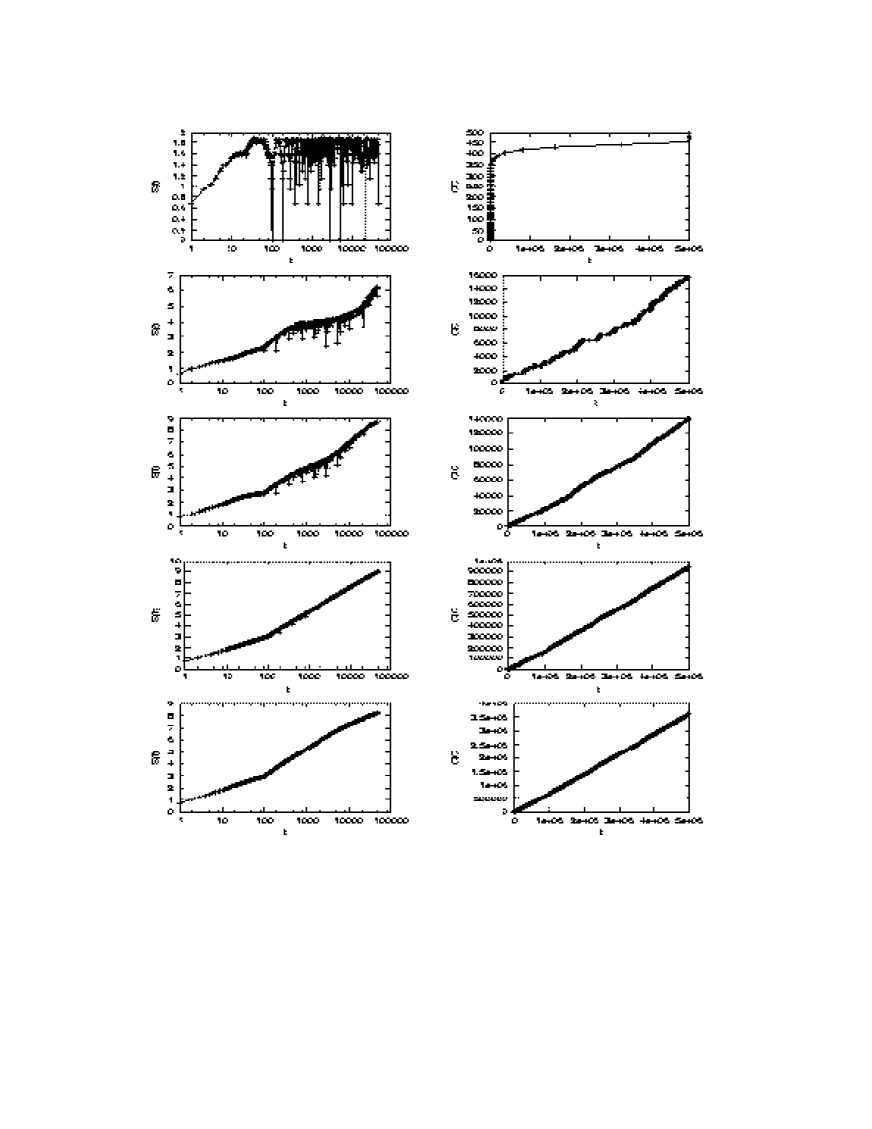
Figure 6: Periodic signal plus noise (see text for details). The figures in the first column refer to the CASSANDRA experiment, while the ones in the second column refer to CASToRe. Figures on the same raw refer to the same value of $\epsilon$, and in particular, from top to bottom $\epsilon=10^{-7},10^{-5},10^{-4},10^{-3},10^{-2}$.

A B

Figure 7: Local indicators of non-random prroperties. A: the local CIC parallels the value of $\epsilon$. B: the CASSANDRA local indicator $I$ has its maximum value when the derivative of $\epsilon$ with respect to time is maximum

7 Events and Pseudo Events

In Section IV we have pointed out what do we mean by event. This definition of event, as an unpredictable random event, implies that we regard as pseudo events the events that are, to some extent to clarify, predictable. Let us illustrate the distinction between events and pseudo events with the help of the dynamic model of Section IV. Let us write it in a more general form, as follows.

$$\dot{x}=\Phi(x)>0,$$ (34)

where $x$ denotes the coordinate of a particle, moving within the interval $I\equiv[0,1]$, from the left to the right, with times of arrival at $x=1$ determined by Eq.(34) and by the initial condition. When the particle reaches the right border of $I$, it is injected back to a new initial condition selected with uniform probability on $I$. Consequently, the times of arrival at $x=1$, $t_{1},..,t_{i}..,$ represent events. As shown in Section IV, the choice $\Phi(x)=\kappa x^{z}$,with $z>1$ and $k>0$, yields for the waiting times $\tau_{i}\equiv t_{i}-t_{i-1}$ the waiting distribution density of Eq. (17).

Next, we convert the time series $\{\tau_{i}\}$ into a random walk. We select a rule [28] that makes the random walker move, always in the same direction and by a step of constant intensity, only when an event occurs. This means that the sequence $\{\tau_{i}\}$ is converted into a sequence of $0$’s and $1$’s as follows. We take the integer part of $\tau_{1}$, say $n_{1}$, and we fill the first $n_{1}$ sites of the sequence with $0$’s. We assign the symbol $1$ to the $n_{1}+1-th$ site and we move to $\tau_{2}$, and so on. The resulting sequence is formed by attaching patches together in the same order as the sequence of $\tau_{i}$. The resulting sequence has a number of sites, say $N$, given by the sum of the integer parts of $\tau_{i}$’s. Then, this resulting sequence is converted into many trajectories of a given length $l$. A window of size $l$ moves along the sequence and for any window position, the portion of the whole sequence spanned by the window is regarded as a single trajectory of length $l$. Thus we obtain $N+1-l$ trajectories that are assumed to start from the origin, and are used to create a diffusion distribution, at time $l$. If there is scaling, the DE method detects it by means of Eq. (14).

The numerical evaluation of $\delta$ with the DE method has been recently done in Ref. [36] and the numerical result supports the theoretical prediction according to which, in the specific case where Eq.(17) applies, the scaling parameter $\delta$, for $2<\mu<3$, reads

$$\delta=\frac{1}{\mu-1}\mbox{ }(\delta=0.5\mbox{ if }\mu>3).$$ (35)

This prediction is known [28] to be correct, only when an ordinary form of memory exists [10]. A Markov master equation, namely a stochastic process without memory, is characterized by a waiting time distribution $\psi(\tau)$ with an exponential form. This implies that a marked deviation from the exponential condition, and thus from $\delta=0.5$, is a signature of the presence of memory[10]. We refer to this memory as Type 1 memory. To illustrate Type 2 memory, we discuss a dynamic model generating both events and pseudo events. For this purpose let us consider a two-variable model. The equation referring to the first variable, is given by Eq.(34), and the one concerning the new variable $y$, is given by

$$\dot{y}=\chi(y)>0.$$ (36)

The variables $x$ and $y$ are the coordinates of two particles, both moving in the interval $I$, always from the left to the right. The initial conditions of the variable $y$ are always chosen randomly. The initial conditions of $x$, on the contrary, are not always chosen randomly, but they are only when the variable $y$ reaches the border at least once, during the sojourn of $x$ within the interval. Let us consider the sojourn time interval $[t_{i},t_{i+1}]$. The times $t_{i}$ signal, as in the case of the earlier 0ne-dimensonal model, the arrival of the particle of interest at $x=1$. If in this time interval the variable $y$ remains within the interval, without touching the right border, then we set $x(t_{i+1})=x(t_{i})$.This means that the next waiting time is equal to the preceding one, and consequently the time $t_{i+2}$, which might be predicted, represents a pseudo event. A random even, or event, occurs when the randomj extraction for the initial condition of $y$ is made. Thus, the sequence $\{t_{i}\}$ reflects a mixture of events and pseudo events. Let us consider the case where $\chi(y)=k^{\prime}y^{z^{\prime}}$ with $z^{\prime}>1$and $k^{\prime}>0$, so as to produce the power index $\mu^{\prime}=z^{\prime}/(z^{\prime}-1)$, with $\mu^{\prime}>2$, a property of real events. Let us set the condition $\langle\tau\rangle_{x}\ll\langle\tau\rangle_{y}$. In this case, it is possible to prove with intuitive arguments that the waiting time distribution of $x$ of Eq.(17) is changed into one much faster than the original. In fact, if we imagine a succession of waiting times for $y$, all equal to $<\tau>_{y}$, we see that the number of long waiting times for $x$ is less than the number of short waiting times, thereby making the perturbed waiting time distribution faster than the original distribution. Let us consider the case where the unperturbed waiting time distribution $\psi(\tau)$ is characterized by $\mu>3$ ($\mu=5$, in the case of Fig. 1). The perturbed waiting time distribution, to be identified with that experimentally observed, is even faster and consequently is expected to produce a diffusion process with $\delta=0.5$. However, the experimental $\psi(\tau)$ is not simply a reflection of real events but includes pseudo events as well. Fig. 8 reveals a very attractive property: the DE now yields $\delta=1/(\mu^{\prime}-1)$, quite different from the prescription of Eq. (35) that would yield $\delta=0.5$. The breakdown of Eq.(35) is a manifestation of Type 2 memory, referred to by us as memory beyond memory. In fact, the existence of pseudo events implies correlation among different times of the series $\{\tau_{i}\}$, and thus a memory of earlier events. The inset of Fig. 8 shows that shuffling the order of the corresponding patches has the effect of yielding $\delta=0.5$, as the experimental $\psi(\tau)$ implies. The scaling detected by the DE method does not depend on the pseudo events, but only on the hidden events, and thus on a time distribution, which cannot be experimentally detected, longer than $\psi(\tau)$.

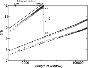
Figure 8: DE for two-variables model as a function of time. The squares correspond to $k^{\prime}$=0.018, $z^{\prime}$=1.83 while the diamonds to $k^{\prime}$=0.011, $z^{\prime}$=1.71. For both curves $k$=0.4, $z$=1.25. Lines correspond to $\delta=0.83$ (full line) and $\delta=0.71$ (dashed line). In the inset: the same curves after shuffling, the straight line slope is $0.5$.

In order to interpret this model via the CIC method, let us consider its discrete version:

$$\left\{\begin{array}[]{ll}y_{n+1}=y_{n}+k^{\prime}\ y_{n}^{z^{\prime}}\Delta t&\mbox{if }0<y_{n}<1\\ y_{n+1}=\Xi_{1}&\mbox{otherwise}\\ w_{n+1}=(1-H(y_{n}-1))w_{n}+H(y_{n}-1)\Xi_{2}\\ x_{n+1}=x_{n}+k\ x_{n}^{z}\Delta t&\mbox{if }0<x_{n}<1\\ x_{n+1}=w_{n}&\mbox{otherwise}\end{array}\right.$$

where $H(s)$ is a Heaviside function, $\Xi_{1}$ and $\Xi_{2}$ are two independent random injections and the function $w_{n}$ is a control on the initial position of $x_{n}$. Note that in the numerical calculation we set the time step $\Delta t=1$.

This way, the system gets an additional degree of freedom (the action of $y_{n}$). Thus, we expect that the KS entropy depends only on the $y_{n}$-dynamics. Hence, the resulting entropy can be compared to the one arising from the formula (23) (with the current value of $z^{\prime}$). The above quantity (23) needs a factor $2=\log_{2}(2^{2})$ correction, due to the increase in one degree of freedom from the one-walker to the two-walkers model: this way we can calculate the entropy using the theory. We have performed two numerical simulations; the results agree with this prediction in both cases where $z=1.25,\ k=0.4,\ z^{\prime}=1.71,\ k^{\prime}=0.011$ and $z=1.25,\ k=0.4,\ z^{\prime}=1.83,\ k^{\prime}=0.018$. In the following table we show that the numerical results obtained using CASToRE fit this prediction.

$z$ value	$k$ value	$z^{\prime}$ value	$k^{\prime}$ value	Theoretical entropy	CASToRe entropy
1.25	0.4	1.71	0.011	0.050	0.053
1.25	0.4	1.83	0.018	0.055	0.058

8 Quasiperiodic Processes

Figure 9: The results of DE analysis for the logistic map at the chaos threshold $x_{n+1}=1-\mu\ x_{n}^{2}$, where the parameter value is $\mu=1.40115518909205$.

This section is devoted to illustrate a dynamic case of significant interest, the logistic map at the chaos threshold. This case is judged to be by many researchers as a prototype of complex systems, for which some other researchers propose the adoption of non-additive entropic indicator[7]. According to the authors of Ref.[14], this case yields an increase of AIC (and CIC) proportional to the logarithm of the window size, namely, a behavior identical to that discussed in Section V. It is therefore of crucial importance to check this prediction by means of CASSANDRA. We have seen that in the periodic case CASSANDRA yields entropy saturation and recurrences, thereby suggesting that the logarithmic increase of AIC does not have a thermodynamic significance, and that the adoption of thermodynamic arguments, non-extensive[7] as well as ordinary, does not seem to be appropriate. It has been recently shown [21] that the adoption of the Pesin theorem yields the same logarithmic dependence on time of the complexity increase, in line with the prediction of Ref.[14]. On the basis of all this, we expect CASSANDRA to result in saturation and recurrences. We see from Fig. 9 that it is so, the only main difference with the case discussed in Section V being that now the recurrences rather than being regular looks erratic.

9 Concluding remarks

From a conceptual point of view, the most important result of this paper is that it sheds light on the connection between scaling and information content, and through the latter, with thermodynamics. This is an important problem since in literature there seems to be confusion on this intriguing issue, insofar as anomalous diffusion is often interpreted in terms of non-ordinary thermodynamics (see, for example [39]). On the contrary, we find that the intermittent model of Section 4 yields an ordinary increase of the information content $I$ as a function of $n$, namely, an increase proportional to $n$ in the whole range $2<\mu<3$. At the diffusion level, this corresponds to the anomalous scaling of Eq. (35). This is the dynamical region corresponding to the emergence of Lévy statistics [3]. Yet, no anomaly is revealed by the measurement of $I$ carried out by means of CASToRE. This seems to fit the conclusion that, after all, Lévy statistics is not incompatible with ordinary statistical mechanics even if it implies a striking deviation from the canonical equilibrium disrribution [17]. It must be pointed out that in the case when the flight perspective is adopted [28, 29] the scaling value $\delta$ keeps obeying the prescription of Eq. (35) even if the condition $\mu<2$ applies. This means that in that case CASSANDRA keeps signalling the existence of scaling even if the exponential sensitivity is replaced by stretched exponential sensitivity.

A more significant property seems to be given by the case when the information content increase becomes proportional to $\log n$. In this specific case, concerning both the periodic case of Fig. 1 and the quasi-periodic case of Fig. 8, the DE cannot exceed a maximum value and is characterized by either periodic (Fig.1) or quasi periodic(Fig. 8) regressions to the initially vanishing value. This means, in other words, again in conflict with Ref. [39], that in this case we are not in the presence of a thermodynamic regime, but rather we are forcing a periodic or quasi-periodic process to generate diffusion. The adoption of moving windows of size $l$ to generate distinct trajectories corresponds, in the periodic case, to producing many trajectories with an unknown initial condition, thereby explaining why we observe initially an entropy increase. Then, the DE undergoes infinitely many regressions signalling to us that this form of entropy increase depends only on the uncertainty on initial condition, rather than on the trajectory complexity. The quasi-periodic case (see Fig. 8) exhibits similar properties, but the initial regime of entropy increase does not seem to exist, in this case.

We are not in the presence of a new thermodynamic regime, and our conclusion should be compared to those of Refs. [37, 38]. These authors prove that strange kinetics do not conflict with ordinary thermodynamics, in the sense that strange kinetics can be comptible with canonical equlilbrium. In our dynamic perspective, thermodynamics means Kolmogorov complexity, and it is in this sense that we agree with the authors of Refs. [37, 38]. We think that strange kinetics do not conflict with the view established by Kolmogorov, and pursued by Pesin, on the basis of the ordinary Shannon entropy. We do not think that anomalous diffusion requires non-ordinary thermodynamics. Rather, anomalous diffusion seems to imply a transition from the dynamic to the thermodynamic regime that might be exceptionally extended in time. For this reason the adoption of the two mobile windows of Section V is expected to afford a powerful method of analysis of time series corresponding to real complex processes. In fact, the two techniques, both CASToRE and CASSANDRA, can be used to explore local time conditions. If the rules driving the dynamics process under study, through the statistical analysis of the sequences generated by the process, change in time, there might be no time for the scaling (thermodynamic) regime to emerge. In this condition, the two techniques can be used to study the transition from dynamics to thermodynamics, a transition never completed due to the fact that the rules change before the realization of the thermodynamic regime occurs.

References

- [1] P. Allegrini, M. Barbi, P. Grigolini and B.J. West, DYNAMICAL MODEL FOR DNA SEQUENCES, Phys. Rev. E 52, (1995), 5281-5296.
- [2] P. Allegrini, P. Grigolini, P. Hamilton, L. Palatella, G. Raffaelli, M. Virgilio, FACING NON-STATIONARY CONDITIONS WITH A NEW INDICATOR OF ENTROPY INCREASE: THE CASSANDRA ALGORITHM, Emergent Nature, M.M. Novak (ed.) World Scientific, 183-184 (2001) ; arXiv:cond-mat/0111246.
- [3] P. Allegrini, P. Grigolini, B.J. West, DYNAMICAL APPROACH TO LEVY PROCESSES, Phys. Rev. E 54 (1996) 4760-4767.
- [4] M. Annunziato, P. Grigolini, STOCHASTIC VERSUS DYNAMIC APPROACH TO LEVY STATISTICS IN THE PRESENCE OF AN EXTERNAL PERTURBATION, Phys. Lett. A 269 (2000) 31-39.
- [5] G. Aquino, P. Grigolini, N. Scafetta, SPORADIC RANDOMNESS, MAXWELL’S DEMON AND THE POINCARE RECURRENCE TIMES, Chaos, Solitons and Fractals, 12, (2001) 2023-2038.
- [6] F. Argenti, V. Benci, P. Cerrai, A. Cordelli, S. Galatolo, G. Menconi, INFORMATION AND DYNAMICAL SYSTEMS: A CONCRETE MEASUREMENT ON SPORADIC DYNAMICS, Chaos, Solitons & Fractals, Vol. 13 (3) (2002), 461-469.
- [7] M. Baranger, V. Latora and A. Rapisarda, TIME EVOLUTION OF THERMODYNAMIC ENTROPY FOR CONSERVATIVE AND DISSIPATIVE CHAOTIC MAPS, Chaos,Solitons,& Fractals, Volume 13, Issue 3, (2002) 471-478.
- [8] Y. Bar-Yam, “Dynamics of Complex Systems”, Addison-Wesley, Reading Mass, (1997).
- [9] C. Beck, F. Schlögl, “Thermodynamics of Chaotic Systems : An Introduction”, Cambridge Nonlinear Science, Cambridge (1993).
- [10] D. Bedeaux, L. Lakatos Lindenberg, K.E. Shuler, ON THE RELATION BETWEEN MASTER EQUATION AND RANDOM WALKS AND THEIR SOLUTIONS, J. Math. Phys. 12, (1971), 2116.
- [11] V. Benci, C. Bonanno, S. Galatolo, G. Menconi, F. Ponchio, INFORMATION, COMPLEXITY AND ENTROPY: A NEW APPROACH TO THEORY AND MEASUREMENTS METHODS, (2001) to appear, http://arXiv.org/abs/math.DS/0107067.
- [12] M. Bologna,. P. Grigolini, M. Karagiorgis and A. Rosa, TRAJECTORY VERSUS PROBABILITY DENSITY ENTROPY, Phys. Rev. E 64, (2001), 016223 (1-9) .
- [13] C. Bonanno,THE MANNEVILLE MAP: TOPOLOGICAL, METRIC AND ALGORITHMIC ENTROPY, (2001),http://arXiv.org/abs/math.DS/0107195 .
- [14] C. Bonanno, G. Menconi, COMPUTATIONAL INFORMATION FOR THE LOGISTIC MAP AT THE CHAOS THRESHOLD, arXiv E-print no. nlin.CD/0102034 (2001), to appear in Discrete and Continuous Dynamical Systems B.
- [15] A. A. Brudno, ENTROPY AND THE COMPLEXITY OF A DYNAMICAL SYSTEM, Trans. Moscow Math. Soc. 2, (1983) 127–151.
- [16] M. Buiatti, P. Grigolini, L. Palatella, A NONEXTENSIVE APPROACH TO THE ENTROPY OF SYMBOLIC SEQUENCES, Physica A, 268, (1999) 214–224.
- [17] M. Bologna, M. Campisi, P. Grigolini. DYNAMIC VERSUS THERMODYNAMIC APPROACH TO NON-EQUIIBRIUM, arXiv: cond-mat/0108361.(2001), in press on Physica A.
- [18] G. J. Chaitin, “Information, randomness and incompleteness. Papers on algorithmic information theory”, World Scientific, Singapore (1987).
- [19] J.R. Dorfman, “An Introduction to Chaos in Nonequilibrium Statistical Mechanics”, Cambridge Lecture Notes in Physics, Cambridge University Press, Cambridge (1999).
- [20] L. Fronzoni, P. Grigolini, S. Montangero, NONEXTENSIVE THERMODYNAMICS AND STATIONARY PROCESSES OF LOCALIZATION, Chaos, Solitons, & Fractals, Volume 11, Issue 14, (2000), 2361-2369.
- [21] L. Fronzoni, S. Montangero, P. Grigolini, THE COMPLEXITY OF THE LOGISTIC MAP AT THE CHAOS THRESHOLD, Physics Letters A, Volume 285, Issues 1-2, (2001) 81-87.
- [22] S. Galatolo,ORBIT COMPLEXITY AND DATA COMPRESSION, Discrete and Continuous Dynamical Systems 7, (2001) 477-486.
- [23] S. Galatolo,ORBIT COMPLEXITY BY COMPUTABLE STRUCTURES, Nonlinearity 13,(2000) 1531-1546.
- [24] S. Galatolo, ORBIT COMPLEXITY, INITIAL DATA SENSITIVITY AND WEAKLY CHAOTIC DYNAMICAL SYSTEMS, arXiv E-print no. math.DS/0102187 (2001).
- [25] S. Galatolo, POINTWISE INFORMATION ENTROPY FOR METRIC SPACES, Nonlinearity 12, 1289-1298 (1999).
- [26] P. Gaspard, X.J. Wang, SPORADICITY: BETWEEN PERIODIC AND CHAOTIC DYNAMICAL BEHAVIOR, Proc. Natl. Acad. Sci. USA 85, (1988) 4591-4595.
- [27] T. Geisel, S. Thomae, ANOMALOUS DIFFUSION IN INTERMITTENT CHAOTIC SYSTEMS, Phys. Rev. Lett. 52, 1936 (1984).
- [28] P. Grigolini, L. Palatella, G. Raffaelli, ASYMMETRIC ANOMALOUS DIFFUSION: AN EFFICIENT WAY TO DETECT MEMORY IN TIME SERIES, Fractals 9 (2001) 193-208.
- [29] P. Grigolini, D. Leddon, N. Scafetta, DIFFUSION ENTROPY AND WAITING TIME STATISTICS OF HARD X-RAY SOLAR FLARES, cond-mat/0108229 (2001).
- [30] M. Ignaccolo, P. Grigolini, A. Rosa, SPORADIC RANDOMNESS: THE TRANSITION FROM THE STATIONARY TO THE NONSTATIONARY CONDITION, Phys. Rev. E 64, 026210 (2001).
- [31] B. B. Mandelbrot, “Fractal Geometry of Nature”, W.H. Freeman Co. (1988).
- [32] P. Manneville, INTERMITTENCY, SELF SIMILARITY AND SPECTRUM IN DISSIPATIVE DYNAMICAL SYSTEMS, J. Physique 41, (1980) 1235-43.
- [33] C.-K. Peng, S.V. Buldyrev, S. Havlin, M. Simons, H.E. Stanley, and A.L. Goldberger, MOSAIC ORGANISATION OF DNA NUCLEOTIDES, Phys. Rev. E 49, (1994) 1685.
- [34] C.-K. Peng, S. Havlin, H.E. Stanley, A.L. Goldberger, QUANTIFICATION OF SCALING EXPONENTS AND CROSSOVER PHENOMENA IN NONSTATIONARY HEARTBEAT TIME SERIES, Chaos 5 (1995), 82–87.
- [35] N. Scafetta, P. Hamilton, P. Grigolini, THE THERMODYNAMICS OF SOCIAL PROCESSES: THE TEEN BIRTH PHENOMENON, Fractals, 9, (2001), 193–208.
- [36] N. Scafetta, V. Latora, P. Grigolini, LEVY STATISTICS IN CODING AND NONCODING DNA, cond-mat/0105041 (2001).
- [37] I.M. Sokolov, THERMODYNAMICS AND FRACTIONAL FOKKER-PLANCK EQUATIONS, Phys. Rev. 63 (2001) (0566111-1)-(056111-8).
- [38] I.M. Sokolov, J. Klafter, and A. Blumen, DO STRANGE KINETICS IMPLY UNUSUAL THERMODYNAMICS?, Phys. Rev. E 64 (2001) (021107-1)-(021107-4).
- [39] C. Tsallis, ENTROPIC NONEXTENSIVITY:A POSSIBLE MEASURE OF COMPLEXITY, Chaos, Solitons & Fractals, 13 , (2002) 371-391.