A novel method to create a vortex in a Bose-Einstein condensate

Abstract

It has been shown that a vortex in a BEC with spin degrees of freedom can be created by manipulating with external magnetic fields. In the previous work, an optical plug along the vortex axis has been introduced to avoid Majorana flips, which take place when the external magnetic field vanishes along the vortex axis while it is created. In the present work, in contrast, we study the same scenario without introducing the optical plug. The magnetic field vanishes only in the center of the vortex at a certain moment of the evolution and hence we expect that the system will lose only a fraction of the atoms by Majorana flips even in the absence of an optical plug. Our conjecture is justified by numerically solving the Gross-Pitaevskii equation, where the full spinor degrees of freedom of the order parameter are properly taken into account. A significant simplification of the experimental realization of the scenario is attained by the omission of the optical plug.

I Introduction

Alkali atoms become a superfluid upon Bose-Einstein condensation (BEC) [1, 2]. The superfluid properties of the system were considered to be essentially the same as those of superfluid ⁴He, in spite of the fact that the former is a weakly-coupled system while the latter is coupled strongly. In contrast with ⁴He, however, alkali atoms have internal degrees of freedom attributed to the hyperfine spin $F$ and, accordingly, the order parameter has $2|F|+1$ components [3, 4]. The atoms ²³Na and ⁸⁷Rb have $|F|=1$, for example, and their order parameters have three components, similarly to the orbital or the spin part of the superfluid ³He.

These degrees of freedom bring about remarkable differences between the BEC of alkali atoms and that of ⁴He. The hyperfine spin freezes along the direction of the local magnetic field when a BEC is magnetically trapped. If a BEC is trapped optically, on the other hand, these degrees of freedom manifest themselves and various new phenomena, such as the phase separation between the different spin states that have never been seen in superfluid ⁴He, may be observed.

It was suggested in [5] and [6] that a totally new process for formation of a vortex in a BEC of alkali atoms is possible by making use of the hyperfine degrees of freedom to “control” the BEC. Suppose a BEC is confined in a Ioffe-Pritchard trap. Then a vortex state with two units of circulation can be continuously created from the vortex free superfluid state by simply reversing the axial magnetic field $B_{z}$, parallel to the Ioffe bars. This field is created by a set of pinch coils and can be easily controlled. Four groups have already reported the formation of vortices with three independent methods [7-11]. Our method is totally different from the previous ones in that the hyperfine spin degrees of freedom have been fully utilized. The present paper is a sequel to [6]. Here, we conduct further investigations on the formation of a vortex by reversing the axial field $B_{z}$. An optical plug along the axis was introduced in [5] and [6] to avoid possible Majorana flips near the axis, that may take place when $B_{z}$ passes through zero. It is expected, however, that trap loss due to Majorana flips may not be very significant if the “dangerous point” $|B|=0$ is passed fast enough and that considerable amount of the BEC remains in the trap as the result. This process should not be too fast, however, such that the adiabatic condition is still satisfied. It is a very difficult task to introduce a sharply forcused optical plug along the center of the condensate whose radius is of the order of a few microns. Accordingly we expect that experimental realization of our scenario will be much easier without the optical plug. In the present paper, therefore, we analyze our scenario by numerically integrating the multi-component Gross-Pitaevskii equation.

This paper is organized as follows. In Sec. II, we outline the order parameter and the Gross-Pitaevskii equation for an $|F|=1$ BEC. In Sec. III, the Gross-Pitaevskii equation is integrated numerically to analyze the time dependence of the order parameter. It will be shown that merely half of the condensate is lost from the trap if the time dependence of the external magnetic field is chosen properly. Sec. IV is devoted to conclusions and discussions. In the Appendix, it is shown that the formation of a vortex in the present scenario may be understood in terms of the Berry phase.

II Order Parameter and Gross-Pitaevskii Equation of $|F|=1$ BEC

Let us briefly summarize the order parameter and the Gross-Pitaevskii equation for a BEC with the hyperfine spin $F=1$ to make this paper self-contained. The readers should be referred to [3] and [6] for further details.

The order parameter of a BEC with $|F|=1$ has three components $\Psi_{i}\ (i=-1,0,+1)$ with respect to the basis vectors $|i\rangle$ defined by $F_{z}|i\rangle=i|i\rangle$. The order parameter $|\Psi\rangle$ is then expanded as

$$|\Psi\rangle=\sum_{i=0,\pm 1}\Psi_{i}|i\rangle.$$

It turns out, however, that another set of basis vectors $|a\rangle\ (a=x,y,z)$, defined by $F_{a}|a\rangle=0$, is more convenient for certain purposes. The order parameter is now expressed as

$$|\Psi\rangle=\sum_{a=x,y,z}\Psi_{a}|a\rangle.$$

The transformation matrix from $\{\Psi_{i}\}$ to $\{\Psi_{a}\}$ is found in [6].

The most general form of the Hamiltonian for $|F|=1$ atoms, that is rotationally invariant except for the Zeeman term, is

$$\hat{H}-\mu\hat{N} = \int\Big{[}\psi^{\dagger}_{a}\left(-\frac{\hbar^{2}}{2m}\nabla^{2}-\mu\right)\psi_{a}+\frac{g_{1}}{2}(\psi^{\dagger}_{a}\psi_{a})^{2}$$ (1)

$$+\frac{g_{2}}{2}|\psi_{a}\psi_{a}|^{2}+i\varepsilon_{abc}\omega_{Lc}\psi^{\dagger}_{a}\psi_{b}\Big{]}d^{3}\mbox{\boldmath$r$},$$

where $\hbar\omega_{La}=\gamma_{\mu}B_{a}$, $\gamma_{\mu}\simeq\mu_{B}/2$ being the gyromagnetic ratio of the atom. The coupling constants are given by

$$g_{1}=\frac{4\pi\hbar^{2}}{m}a_{2},\quad g_{2}=\frac{4\pi\hbar^{2}}{m}\frac{a_{0}-a_{2}}{3},$$ (2)

where $a_{2}=2.75\;\mathrm{nm}$ and $a_{0}=2.46\;\mathrm{nm}$ [12].

The Heisenberg equation of motion derived from the above Hamiltonian is

$$i\hbar\frac{\partial\psi_{a}}{\partial t} = [\psi_{a},\hat{H}-\mu\hat{N}]$$ (3)

$$= \left(-\frac{\hbar^{2}}{2m}\nabla^{2}-\mu\right)\psi_{a}+g_{1}(\psi^{\dagger}_{b}\psi_{b})\psi_{a}$$

$$+g_{2}(\psi_{b}\psi_{b})\psi_{a}^{\dagger}+i\varepsilon_{abc}\omega_{Lc}\psi_{b}.$$

By taking the expectation value of the above equation in the mean-field approximation, $\langle\psi\psi\psi\rangle\simeq\Psi\Psi\Psi$, where $\Psi_{a}=\langle\psi_{a}\rangle$, we obtain

$$i\hbar\frac{\partial\Psi_{a}}{\partial t} = \left(-\frac{\hbar^{2}}{2m}\nabla^{2}-\mu\right)\Psi_{a}+g_{1}|\Psi|^{2}\Psi_{a}$$ (4)

$$+g_{2}(\Psi)^{2}\Psi^{*}_{a}+i\varepsilon_{abc}\omega_{Lc}\Psi_{b}.$$

This is the fundamental equation which we will use in the rest of this paper.

III Creation of a Vortex

III.1 Magnetic Fields

Suppose we confine a BEC in a Ioffe-Pritchard trap with a quadrupole magnetic field

$$\mbox{\boldmath$B$}_{\perp}(\mbox{\boldmath$r$})=\left(\begin{array}[]{c}B_{\perp}(r)\cos(-\phi)\\ B_{\perp}(r)\sin(-\phi)\\ 0\end{array}\right)$$ (5)

and a uniform axial field

$$\mbox{\boldmath$B$}_{z}(t)=\left(\begin{array}[]{c}0\\ 0\\ B_{z}(t)\end{array}\right).$$ (6)

Here $(r,\phi,z)$ are the cylindrical coordinates. The magnitude $B_{\perp}(r)$ is proportional to $r$ near the axis $r\sim 0$; $B_{\perp}(r)\simeq B^{\prime}r$, with $B^{\prime}$ being a constant. The system is assumed to be uniform along the $z$ direction for calculational simplicity. Our analysis should apply to a cigar-shaped system as well.

Suppose we reverse the $\mbox{\boldmath$B$}_{z}$ field slowly, while keeping $\mbox{\boldmath$B$}_{\perp}$ fixed as shown in Fig. 1. It was shown in [5, 6] that a vortex with two units of circulation will be formed if we start with a vortex-free BEC. In these papers, an optical plug was introduced along the vortex axis to prevent the atoms from escaping from the trap when $\mbox{\boldmath$B$}=\mbox{\boldmath$B$}_{\perp}+\mbox{\boldmath$B$}_{z}$ vanishes at $r=0,t=T/2$. Accordingly, the order parameter remains within the weak-field seeking state (WFSS) throughout the scenario.

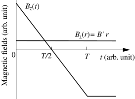
Figure 1: The schematic time dependence of the axial field $B_{z}$. The field $B_{z}$ reverses the sign in an interval of time $T$, while the quadrupole field $\mbox{\boldmath$B$}_{\perp}=B^{\prime}r$ remains fixed. The field $B_{z}(t)$ is fixed at the value $B_{z}(T)=-B_{z}(0)$ for $t>T$ for further evolution.

We suspect, however, that the BEC may be stable even without the optical plug since $B$ vanishes only in $r=0$ at the time $t=T/2$. This will be justified by solving the Gross-Pitaevskii equation numerically below. In contrast with the previous work, we have to take the full degrees of freedom of the order parameter into account since the energies of the three hyperfine states (the strong-field seeking state, the weak-field seeking state and the neutral state) are degenerate when $\mbox{\boldmath$B$}=0$.

III.2 Initial State

We first solve the Gross-Pitaevskii equation in the stationary state to find the initial order parameter configuration and the corresponding chemical potential. There is a sufficient gap between the weak-field seeking state and the other states at $t=0$ and the BEC may be assumed to be purely in the weak-field seeking state. Let us parametrize the external magnetic field $B$ with use of the polar angles $\alpha$ and $\beta$ as

$$\mbox{\boldmath$B$}(r,t)=\mbox{\boldmath$B$}_{\perp}(r)+\mbox{\boldmath$B$}_{z}(t)=|\mbox{\boldmath$B$}|\left(\begin{array}[]{c}\sin\beta\cos\alpha\\ \sin\beta\sin\alpha\\ \cos\beta\end{array}\right),$$ (7)

where $\alpha=-\phi$ for the quadrupole field and

$$\beta=\tan^{-1}\left[\frac{|\mbox{\boldmath$B$}_{\perp}(r)|}{|\mbox{\boldmath$B$}_{z}(t)|}\right].$$ (8)

Since the hyperfine spin $F$ is antiparallel with $B$, we must have

$$\hat{\mbox{\boldmath$l$}}=\left(\begin{array}[]{c}-\sin\beta\cos\alpha\\ -\sin\beta\sin\alpha\\ -\cos\beta\end{array}\right),$$ (9)

where $\hat{\mbox{\boldmath$l$}}$ is a unit vector parallel to $F$, see Fig. 2.

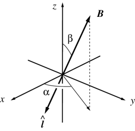
Figure 2: Polar angles $(\alpha,\beta)$ parametrizing $B$ and $\hat{\mbox{\boldmath$l$}}\parallel\mbox{\boldmath$F$}$.

The most general form for the order parameter yielding the above $\hat{\mbox{\boldmath$l$}}$ vector is

$$\Psi_{a}=\frac{f_{0}}{\sqrt{2}}e^{-i\gamma}\left(\begin{array}[]{c}\cos\beta\cos\alpha+i\sin\alpha\\ \cos\beta\sin\alpha-i\cos\alpha\\ -\sin\beta\end{array}\right)\equiv f_{0}v_{a},$$ (10)

where $\{v_{a}\}$ represents the “phase”, while $f_{0}$ is the amplitude of the order parameter. In mathematical terms, $\{v_{a}\}$ defines the local $SO(3)$ frame or the “triad” of the real orthonormal vectors $\{\hat{\mbox{\boldmath$m$}},\hat{\mbox{\boldmath$n$}},\hat{\mbox{\boldmath$l$}\}}$, where

$$v_{a}=\frac{1}{\sqrt{2}}e^{-i\gamma}(\hat{\mbox{\boldmath$m$}}+i\hat{\mbox{\boldmath$n$}})_{a},\quad\hat{\mbox{\boldmath$l$}}=\hat{\mbox{\boldmath$m$}}\times\hat{\mbox{\boldmath$n$}}.$$ (11)

It should be noted that the above order parameter takes the same form as that of the orbital part of the superfluid ³He-A.

One may obtain more insight if the order parameter in Eq. (10) is rewritten in the $\Psi_{i}$ basis as [13]

$$\Psi_{i}=f_{0}e^{-i\gamma}\left(\begin{array}[]{c}\frac{1}{2}e^{-i\alpha}(1-\cos\beta)\\ -\frac{1}{\sqrt{2}}\sin\beta\\ \frac{1}{2}e^{i\alpha}(1+\cos\beta)\end{array}\right).$$ (12)

The angle $\beta$ vanishes at $r=0$ (note that $\mbox{\boldmath$B$}_{\perp}=0$ at $r=0$), hence we find $\Psi_{+1}=\Psi_{0}=0$ while $\Psi_{-1}\propto e^{i(\alpha-\gamma)}\neq 0$ there. For the order parameter to be smooth at $r=0$, we have to choose

$$\gamma=\alpha=-\phi.$$ (13)

Accordingly, the order parameter takes the form

$$\Psi_{a}=\frac{f_{0}}{\sqrt{2}}e^{i\phi}\left(\begin{array}[]{c}\cos\beta\cos\phi-i\sin\phi\\ -\cos\beta\sin\phi-i\cos\phi\\ -\sin\beta\end{array}\right)$$ (14)

in the $\Psi_{a}$ basis and

$$\Psi_{i}=\frac{f_{0}}{2}\left(\begin{array}[]{c}(1-\cos\beta)e^{2i\phi}\\ -{\sqrt{2}}\sin\beta e^{i\phi}\\ 1+\cos\beta\end{array}\right)$$ (15)

in the $\Psi_{i}$ basis. It follows from Eq. (15) that the state with $\hat{\mbox{\boldmath$l$}}=-\hat{\mbox{\boldmath$z$}}\ (\beta=0)$ has a vanishing winding number, while that with $\hat{\mbox{\boldmath$l$}}=\hat{\mbox{\boldmath$z$}}\ (\beta=\pi)$ has the winding number $2$. Accordingly, the former state may be continuously deformed to the latter state by changing $\beta$ from $0$ to $\pi$ smoothly, resulting in the formation of a vortex with winding number 2 [14, 15]. It is shown in the Appendix that this phase may also be understood in terms of the Berry phase associated with the adiabatic change of the local magnetic field.

The stationary Gross-Pitaevskii equation is given by

$$-\frac{\nabla^{2}}{2m}\Psi_{a}+g_{1}|\Psi|^{2}\Psi_{a}+g_{2}\Psi^{2}\Psi_{a}^{*}+i\varepsilon_{abc}\Psi_{b}\omega_{Lc}=\mu\Psi_{a}.$$ (16)

By substituting the WFSS order parameter in Eq. (14) into Eq. (16), we obtain

$$-\frac{\hbar^{2}}{2m}\Big{[}\nabla^{2}-\frac{\beta^{\prime 2}}{2}-\frac{1}{4r^{2}}(7-8\cos\beta+\cos 2\beta)\Big{]}f_{0}\qquad$$

$$\qquad\qquad+\gamma_{\mu}B(r)f_{0}+g_{1}f_{0}^{3}=\mu f_{0}.$$ (17)

Note that there appears an extra term $\beta^{\prime 2}$ that is missing if this BEC is described by a scalar (namely $U(1)$) order parameter. This term originates from $v_{a}^{\dagger}\nabla^{2}v_{a}$ and represents the rotation of the local $SO(3)$ frame. In ordinary physical settings, however, this term is smaller than the $B$-term by a factor of $\omega/\omega_{L}\sim 10^{-3}$ and hence its effect may be negligible in the following arguments.

The amplitude of the external magnetic field has an approximately harmonic potential profile near the origin,

$$B(r,t) = \sqrt{B_{\perp}^{2}(r)+B_{z}^{2}(t)}\simeq\sqrt{B^{\prime 2}r^{2}+B_{z}^{2}(t)}$$ (18)

$$\simeq B_{z}(t)+\frac{B^{\prime 2}}{2B_{z}(t)}r^{2}.$$

It turns out to be convenient to scale the energies by the energy-level spacing $\hbar\omega$ at $t=0$ and the lengths by the harmonic-oscillator length $a_{\rm HO}$, where

$$\omega = B^{\prime}\sqrt{\frac{\gamma_{\mu}}{mB_{z}(0)}},$$ (19)

$$a_{\rm HO} = \sqrt{\frac{\hbar}{m\omega}}.$$ (20)

If we take ²³Na and substitute $B_{z}(0)=1\;\mathrm{G}$ and $B^{\prime}=300\;\mathrm{G/cm}$, we find $a_{\rm HO}\sim 9.14\times 10^{-1}\;\mathrm{\mu m}$ and $\hbar\omega\sim 3.49\times 10^{-24}\;\mathrm{erg}$. For the same choice of the parameters, we have $\omega_{L}(r=0,t=0)\sim 4.40\times 10^{6}\;{\mathrm{rad/s}}\sim 1.330\times 10^{3}\omega$. It is reasonable to assume $\tau\equiv 2\pi/\omega_{L}(r=0,t=0)\sim 1.43\;\mathrm{\mu s}$ to be the measure of the adiabaticity.

After these scalings, the dimensionless Gross-Pitaevskii equation takes a simpler form

$$-\frac{1}{2}\tilde{\nabla}^{2}\tilde{f}_{0} + \left[\tilde{B}(r)+\frac{\beta^{\prime 2}}{4}+\frac{1}{8\tilde{r}^{2}}(7-8\cos\beta+\cos 2\beta)\right]\tilde{f}_{0}$$ (21)

$$+\tilde{g}_{1}\tilde{f}_{0}^{3}=\tilde{\mu}\tilde{f}_{0},$$

where $\tilde{r}=r/a_{\rm HO},\tilde{f}_{0}=f_{0}a_{\rm HO}^{3/2},\tilde{\mu}=\mu/\hbar\omega$, $\tilde{B}=\gamma_{\mu}B/\hbar\omega$ and $\tilde{g}_{1}=g_{1}/a_{\rm HO}^{3}\hbar\omega\sim 0.0378$. A similar scaling for $g_{2}$ yields $\tilde{g}_{2}\sim-0.00132$. Note that the singularity at $\tilde{r}=0$ vanishes if $\beta(\tilde{r})$ approaches to 0 fast enough as $\tilde{r}\to 0$. The tildes will be dropped hereafter whenever it does not cause confusion. The eigenvalue $\mu$ may be obtained numerically. For ²³Na with $B_{z}$ and $B^{\prime}$ given above, we find ${\mu}-\hbar\omega_{L}(r=0,t=0)=3.66$, which amounts to $1.28\times 10^{-23}\;{\mathrm{e}rg}$ in dimensional units. Figure 3 shows the corresponding condensate profile $f_{0}(r)$.

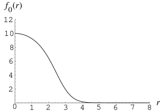
Figure 3: Condensate wave function $f_{0}(r)$. The condensate wave function and the radial coordinate are scaled by $a_{\rm HO}^{-3/2}$ and $a_{\rm HO}$, respectively, and hence dimensionless.

III.3 Time Development

The time development of the condensate wavefunction is obtained by solving the Gross-Pitaevskii Eq. (4) which is written in dimensionless form as

$$i\frac{\partial\Psi_{a}}{\partial t} = -\frac{1}{2}\nabla^{2}\Psi_{a}+g_{1}|\Psi|^{2}\Psi_{a}$$ (22)

$$+g_{2}(\Psi)^{2}\Psi^{*}_{a}+i\varepsilon_{abc}\Psi_{b}\omega_{Lc}.$$

The initial condition is

$$\Psi_{a}=f_{0}(r)v_{a},$$ (23)

where $f_{0}(r)$ is obtained in the previous subsection and $v_{a}$ is defined in Eq. (10). The condensate cannot remain within the weak-field seeking state during the formation of a vortex and we have to utilize the full degrees of freedom of the order parameter $\Psi_{a}$. The Gross-Pitaevskii equation has been solved numerically to find the temporal development of the order parameter while $B_{z}$ changes as

$$B_{z}(t)=B_{z}(0)\left[1-\frac{2t}{T}\right]\quad(0\leq t\leq T),$$ (24)

with several choices for the reversing time $T$. Adiabaticity is not guaranteed at $t\sim T/2$ when the energy gaps among the weak-field seeking state (WFSS), the neutral state (NS) and the strong-field seeking state (SFSS) disappear. We expect, however, that this breakdown of adiabaticity is not very significant to the condensate since it takes place only along the condensate axis for a short period of time.

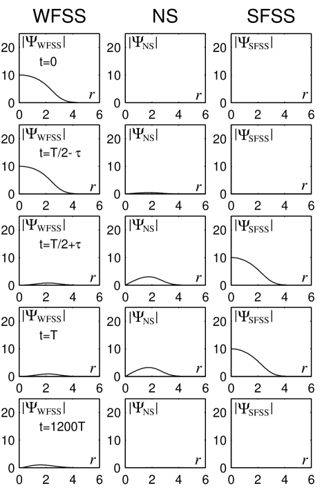
Figure 4: Temporal development of the order parameters $|\Psi_{\rm WFSS}|$, $|\Psi_{\rm NS}|$ and $|\Psi_{\rm SFSS}|$ for $T=10\tau$, where $\tau\sim 1.43\mu{\rm s}$. The graphs are plotted for $t=0$ (initial state), $t=T/2-\tau$ (slightly before $B_{z}=0$ is crossed), $t=T/2+\tau$ (slightly after $B_{z}=0$ is crossed) and $t=T$ ($B_{z}$ is completely reversed). Furthermore, $B_{z}$ is fixed to $B_{z}(T)=-B_{z}(0)$ for $t>T$. The bottom row shows the order parameters at $t=1200T$. The order parameters and the radial coordinate are plotted in units of $a_{\rm HO}^{-3/2}$ and $a_{\rm HO}$, respectively.

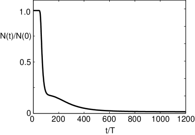
Figure 5: The ratio $N(t)/N(0)$ as a function of $t/T$ for the reversing time $T=10\tau$. Here $N(t)$ is the number of atoms$/$unit length along the vortex axis at time $t$. The magnetic field $B_{z}$ decreases monotonically for $0\leq t/T\leq 1$, but is kept fixed to $-B_{z}(0)$ for $T\leq t$, see Fig. 1.

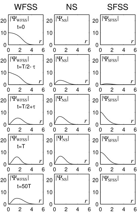
Figure 6: Same as in Fig. 4, but for $T=100\tau$, $\tau\sim 1.43\mu{\rm s}$. The graphs are plotted for $t=0,t=T/2-\tau,t=T/2+\tau,t=T$, and $t=50T$.

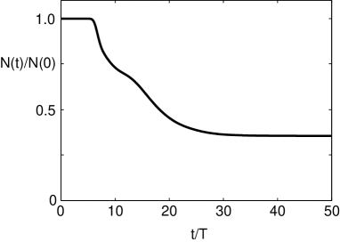
Figure 7: Same as in Fig. 5, but for $T=100\tau$.

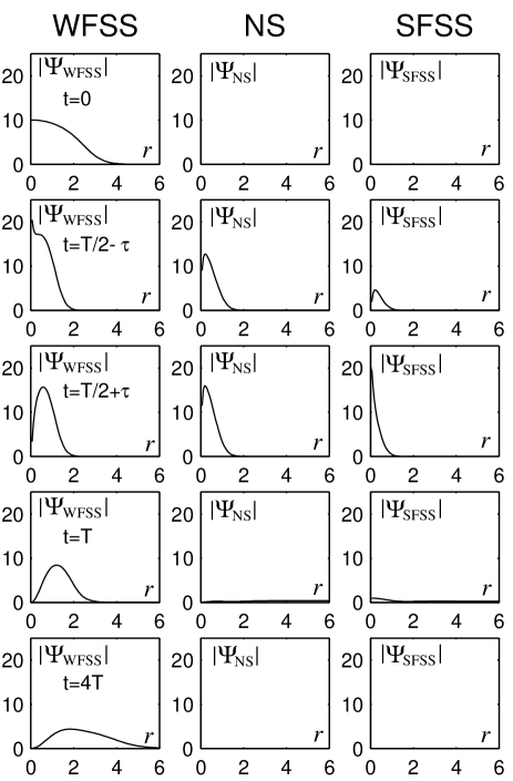
Figure 8: Same as in Fig. 4, but for $T=1000\tau$, $\tau=1.43\mu{\rm s}$. The graphs are plotted for $t=0,t=T/2-\tau,t=T/2+\tau,t=T$, and $t=4T$.

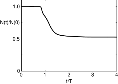
Figure 9: Same as in Fig. 5, but for $T=1000\tau$.

We project $\Psi_{a}$ thus obtained to the local WFSS, NS and SFSS by defining the projection operators to the respective states as

$$\begin{array}[]{c}\Pi_{\rm{W}ab}=v_{a}v_{b}^{\dagger},\quad\Pi_{\rm{S}ab}=u_{a}u_{b}^{\dagger},\vspace{0.3cm}\\ \Pi_{\rm{N}ab}=\delta_{ab}-\Pi_{\rm{W}ab}-\Pi_{\rm{S}ab}\end{array}$$ (25)

where

$$v_{a}=\frac{1}{\sqrt{2}}(\hat{\mbox{\boldmath$m$}}+i\hat{\mbox{\boldmath$n$}})_{a},u_{a}=\frac{1}{\sqrt{2}}(\hat{\mbox{\boldmath$m$}}-i\hat{\mbox{\boldmath$n$}})_{a}$$ (26)

define the local WFSS and SFSS $SO(3)$ frames, respectively.

Figures 4, 6, and 8 depict the amplitudes of the wave functions at $t=0,T/2-\tau,T/2+\tau$ and $T$ for $T=10\tau,100\tau$, and $1000\tau$. Figures 5, 7, and 9 show the particle numbers within the trap for the same choices of $T$. To simulate the trap loss, we introduced a function

$$h(r)=\frac{1}{2}\left[1-\tanh\left(\frac{r-r_{0}}{\lambda}\right)\right],$$ (27)

with $r_{0}=30$ and $\lambda=2$. The wave function $\Psi_{a}(r)$ is multiplied by $h(r)$ after each step of the Crank-Nicholson algorithm. The parameter $r_{0}$ roughly corresponds to the trap size, while $\lambda$ is taken large enough to prevent the wavefunction being reflected at $r\sim r_{0}$. Thus particles that reach beyond $r\sim r_{0}$ disappear from the trap. The parameters $r_{0}$ and $\lambda$ are introduced for purely computational purposes and should not be confused with any realistic experimental settings. As $t\gg T$, the condensates in SFSS and NS disappear from the trap and the particle number reaches its equilibrium value. The bottom row of Figs. 4, 6, and 8 shows the wavefunctions after the equilibrium is attained.

Figure 4 shows the behavior of the condensate when $T=10\tau$. In this case, $B_{z}(t)$ is reversed so fast that most of the particles remain in the WFSS at $t=T/2-\tau$ and they are suddenly converted into the SFSS at $t=T/2+\tau$. These particles in the SFSS and the NS are eventually lost from the trap as $t\to\infty$, see Fig. 5.

Figures 6 and 8 show that the behavior of the condensate is qualitatively similar for $T=100\tau$ and $T=1000\tau$. The condensate is transferred from the WFSS to the SFSS more efficiently at $t=T/2-\tau$ for $T=1000\tau$ which leads to more WFSS components at $t=T/2+\tau$ in this case. At a later time $t>T$, the condensate is found to oscillate in the trap with the frequency $\sim\omega$.

We have also analyzed the case $T=10000\tau$ and found no qualitative difference compared to the case $T=1000\tau$. There are slightly more of the NS component in the former case at $t=T/2-\tau$ than the latter case, which leads to less particles in its equilibrium state at $t\gg T$ .

It is certainly desirable to have more particles remaining in the trap when a vortex is created. Figure 10 shows the ratio of the final particle number to the initial particle number as a function of the reversing time $T$. Note that the final particle number is evaluated when the equilibrium is reached. It is found that a considerable amount of the condensate $(\gtrsim 1/3)$ is left in the trap for a wide range of the reversing times $10^{2}\lesssim T/\tau\lesssim 10^{4}$.

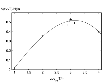
Figure 10: Ratio of the residual particle number to the initial particle number as a function of $\log_{10}(T/\tau)$. The crosses are the results of our numerical calculation while the interpolating curve is introduced as a guide.

In summary, our numerical calculations indicate that a large fraction of the BEC remains in the trap when $B_{z}$ is reversed with proper choices of the reversing time $T$. Although there remain SFSS and NS components at $t=T$, they eventually disappear from the trap at $t\gg T$ when the equilibrium is reached. The condensate is converted into a state with two units of circulation. Thus we conclude that a vortex can be created, even in the absence of an optical plug, by simply reversing the axial field $B_{z}$. We expect that this makes the experimental realization of the present scenario much easier than that with an optical plug [5, 6].

IV Conclusions and Discussions

We have analyzed a simple scenario of vortex formation in a spinor BEC. An axial magnetic field is slowly reversed while the quadrupole field has been kept fixed in a Ioffe-Pritchard trap, which results in a formation of a vortex with the winding number $2$. The spinor degrees of freedom have been fully utilized which renders our scheme much simpler compared with other methods.

Since the vortex thus created has a higher winding number, it is metastable and eventually breaks up to two singly quantized vortices. The lifetime of the metastable state is quite an interesting quantity to evaluate since its magnitude, compared with the field-reversal time $T$ and the trap time, will be crucial to determine the ultimate fate of the vortex.

A similar analysis with an $F=2$ BEC is under progress and will be published elsewhere.

Appendix A Vortex Formation and Berry Phase

It is shown that the formation of a vortex in our scenario is understood from a slightly different viewpoint. Namely, we show that the phase appearing in the end of the process may be identified with the Berry phase associated with the adiabatic change of the magnetic field.

Let a point on the unit sphere in Fig. 11 (a) denote the hyperfine spin state with $F=1$. All the spins near the origin $r=0$ have $F_{z}\simeq-1$ at $t=0$ and hence correspond to the points near the south pole. Now the axial field $B_{z}$ monotonically decreases such that eventually all the spins near the origin have $F_{z}\simeq+1$ at $t=T$ and hence are expressed by the points near the north pole. The path a spin follows on the unit sphere depends on the position of the spin relative to the origin. Figure 11 (b) shows the configuration of four hyperfine spins $F$ at $t=T/2$, when $B_{z}$ vanishes and $F$ is determined by the quadrupole field. The path $C_{1}$ in Fig. 11 (a) shows the trajectory the spin 1 in Fig. 11 (b) follows when $t$ is varied from $0\ (\beta=0)$ to $T\ (\beta=\pi)$. Similarly the path $C_{2}$ in Fig. 11 (a) is the trajectory of the spin 2 in Fig. 11 (b), and so on. When the spins 1 and 2 left the south pole at $t=0$, they had the common phase factor, while at $t=T$ they obtain the relative phase equal to the solid angle subtended by the trajectories $C_{1}$ and $C_{2}$. The shaded area in Fig. 11 (a) shows this area which subtends the solid angle $\pi$. Similarly the paths 1 and 3 (1 and 4) subtend the solid angle $2\pi$ ($3\pi$), resulting in the relative phase $2\pi(3\pi)$ between the spins 1 and 3 (1 and 4), respectively, when $B_{z}$ is completely reversed. Accordingly, as one completes a loop surrounding the origin, one measures the phase change of $4\pi$ observing that a vortex formation has taken place.

Figure 11: Formation of a vortex in the present scenario may be understood in terms of the Berry phase associated with each spin. When $|B_{z}|\gg|B_{\perp}|$ at $t=0$, all the spins near the origin have $F_{z}\simeq-1$ with the same phase. Due to the “twisting” of the spins during the evolution, they obtain different phases depending on the trajectories they follow. (b) shows four spins at $t=T/2$ where $B_{z}$ vanishes. The spin 1 follows the trajectory denoted by $C_{1}$ in (a) starting from the south pole and ending at the north pole. Similarly the spins 2, 3 and 4 in (b) follows the trajectories $C_{2},C_{3}$ and $C_{4}$ in (a), respectively. The shaded area $(\pi/2\leq\phi\leq\pi,0\leq\beta\leq\pi)$ in (a) is the solid angle subtended by the paths $C_{1}$ and $C_{2}$. Since this area measures $\pi$, the spin $2$ has a phase $\pi$ relative to that of the spin $1$ at $t=T$. Similarly the spins 3 and 4 obtain phases $2\pi$ and $3\pi$, respectively, relative to that of the spin 1 at $t=T$.

References

- (1) M. Inguscio, S. Stringari, and C. E. Wieman (eds.), Bose-Einstein Condensation in Atomic Gases, (IOS Press, Amsterdam, 1999).
- (2) S. Martellucci, A. N. Chester, A. Aspect, and M. Inguscio (eds.), Bose-Einstein Condensates and Atomic Lasers, (Kluwer Academic/ Plenum Publishers, New York, 2000).
- (3) T. Ohmi and K. Machida, J. Phys. Soc. Jpn. 67, 1822 (1998).
- (4) T.-L. Ho, Phys. Rev. Lett. 81, 742 (1998).
- (5) M. Nakahara, T. Isoshima, K. Machida, S.-I. Ogawa and T. Ohmi, Physica B 284-288, 17 (2000).
- (6) T. Isoshima, M. Nakahara, T. Ohmi, and K. Machida, Phys. Rev. A 61, 063610 (2000).
- (7) M. R. Matthews, B. P. Anderson, P. C. Haljan, D. S. Hall, C. E. Wieman, and E. A. Cornell, Phys. Rev. Lett. 83, 2498 (1999).
- (8) K. W. Madison, F. Chevy, W. Wohlleben, and J. Dalibard, Phys. Rev. Lett. 84, 806 (2000).
- (9) J. R. Abo-Shaeer, C. Raman, J. M. Vogels, and W. Ketterle, Science 292, 476 (2001).
- (10) E. Hodby, G. Hechenblaikner, S. A. Hopkins, O. M. Marago, and C.J. Foot, Phys. Rev. Lett. 88 010405 (2001).
- (11) P. C. Haljan, I. Coddington, P. Engels, and E. A. Cornell, Phys. Rev. Lett. 87, 210403 (2001).
- (12) D. M. Stamper-Kurn and W. Ketterle: in R. Kaiser, C. Westbrook, F. David (eds.), Coherent atomic matter waves - Ondes de matiere coherentes, (Springer, Heidelberg, 2001).
- (13) K. Maki and T. Tsuneto: J. Low Temp. Phys. 27, 635 (1977).
- (14) P. W. Anderson and G. Toulouse, Phys. Rev. Lett. 38, 508 (1977).
- (15) N. D. Mermin and T.-L. Ho, Phys. Rev. Lett. 36, 594 (1976).