BI-TP 2001/21
May 2002
cond-mat/0202017

Universal amplitude ratios from numerical
studies of the three-dimensional $O(2)$ model
A. Cucchieri$\,{}^{\rm a}$, J. Engels$\,{}^{\rm b}$, S. Holtmann$\,{}^{\rm b}$, T. Mendes$\,{}^{\rm a}$, T. Schulze$\,{}^{\rm b}$

^aIFSC-USP, Caixa postal 369, 13560-970 São Carlos SP, Brazil

^bFakultät für Physik, Universität Bielefeld, D-33615 Bielefeld, Germany

Abstract

We investigate the three-dimensional $O(2)$ model near the critical point by Monte Carlo simulations and calculate the major universal amplitude ratios of the model. The ratio $U_{0}=A^{+}/A^{-}$ is determined directly from the specific heat data at zero magnetic field. The data do not, however, allow to extract an accurate estimate for $\alpha$. Instead, we establish a strong correlation of $U_{0}$ with the value of $\alpha$ used in the fit. This numerical $\alpha$-dependence is given by $A^{+}/A^{-}=1-4.20(5)\alpha+O(\alpha^{2})$. For the special $\alpha$-values used in other calculations we find full agreement with the corresponding ratio values, e. g. that of the shuttle experiment with liquid helium. On the critical isochore we obtain the ratio $\xi^{+}/\xi^{-}_{T}=0.293(9)$, and on the critical line the ratio $\xi_{T}^{c}/\xi_{L}^{c}=1.957(10)$ for the amplitudes of the transverse and longitudinal correlation lengths. These two ratios are independent of the used $\alpha$ or $\nu$-values.

PACS : 64.60.Cn; 75.40.; 05.50+q

Keywords: $O(2)$ model; Universal amplitude ratios; Specific heat; Correlation length

Short title: Universal amplitude ratios of the $3d$ $O(2)$ model

 
E-mail: engels, holtmann, tschulze@physik.uni-bielefeld.de ;
cucchieri, mendes@if.sc.usp.br

1 Introduction

In quantum field theory and condensed matter physics $O(N)$ symmetric vector models play an essential part, because they are representatives of universality classes for many physical systems. The universal properties of the $O(N)$ models - the critical exponents and amplitude ratios, which describe the critical phenomena - are therefore of considerable importance. In three dimensions the case $N=2$ is a special one: it is the first vector model (with increasing $N$) showing Goldstone effects, and the exponent $\alpha$, which controls the critical behaviour of the specific heat, is very close to zero. In fact, if one plots $\alpha$ versus $N$, as determined by field theory methods [1]-[4], then the function is approximately linear in $N$ and becomes negative just below $N=2$. The proximity of $\alpha$ to zero made it also difficult to determine the type of the singularity for the specific heat in real systems. Indeed, for the lambda transition of helium a nearly logarithmic singularity (corresponding to $\alpha=0$) was first measured [5] and a similar behaviour was found at the gas-liquid critical point [6]. However, with the nowadays reached experimental precision, especially that of the spectacular shuttle experiment with liquid helium [7, 8] there is no doubt that the critical exponent $\alpha$ is very small, but non-zero, and because it is negative the peak of the specific heat is finite.

In this paper we calculate, among others quantities, the specific heat from Monte Carlo simulations. The determination of $\alpha$ from these data poses, as we shall see, similar problems as in experiments. Of course, there is only one value of $\alpha$ for the $3d$ $O(2)$-universality class, but it is unclear what the correct value is (see e. g. the survey in Table 19 of Ref. [9]). We therefore pursue the strategy to calculate the universal ratios from our data for different $\alpha$-values in the range where the actual value most probably is. The strongest dependence on the used $\alpha$ is expected for fits involving the universal amplitude ratio $A^{+}/A^{-}$ of the specific heat. The same is true for all theoretical determinations [10, 11] of this ratio. Apart from $A^{+}/A^{-}$ we derive from our simulations other universal quantities and amplitude ratios, which characterize the $O(2)$-universality class in three dimensions.

The model which we investigate is the standard $O(2)$-invariant nonlinear $\sigma$-model (or $XY$ model), which is defined by

$$\beta\,{\cal H}\;=\;-J\,\sum_{<x,y>}\vec{\phi}_{x}\cdot\vec{\phi}_{y}\;-\;{\vec{H}}\cdot\,\sum_{x}\vec{\phi}_{x}\;.$$ (1)

Here $x$ and $y$ are the nearest-neighbour sites on a three-dimensional hypercubic lattice, $\vec{\phi}_{x}$ is a $2$-component unit vector at site $x$ and $\vec{H}$ is the external magnetic field. We consider the coupling constant $J$ as inverse temperature, that is $J=1/T$. Instead of fixing the length of the spin vectors $\vec{\phi}_{x}$ to 1 we could have introduced an additional term $\sum_{x}[\vec{\phi}_{x}^{2}+\lambda(\vec{\phi}_{x}^{2}-1)^{2}]$ on the right hand side of the last equation. By choosing an appropriate $\lambda$ value [12] it is then possible to eliminate leading order corrections to scaling. As it will turn out, these corrections are negligibile in the energy density and marginal in the specific heat also with the Hamiltonian from Eq. (1). Moreover, we want to combine amplitudes obtained from former simulations at non-zero magnetic field [13] using the same Hamiltonian with the amplitudes we determine now in order to calculate universal ratios.

As long as $H=|{\vec{H}}|$ is non-zero one can decompose the spin vector $\vec{\phi}_{x}$ into a longitudinal (parallel to the magnetic field ${\vec{H}}$) and a transverse component

$$\vec{\phi}_{x}\;=\;\phi_{x}^{\parallel}{\vec{e}_{H}}+\vec{\phi}_{x}^{\perp}~{},\quad{\rm with}~{}~{}{\vec{e}_{H}}={\vec{H}}/H~{}.$$ (2)

The order parameter of the system, the magnetization $M$, is then the expectation value of the lattice average $\phi^{\parallel}$ of the longitudinal spin component

$$M\;=\;\langle\>\frac{1}{V}\sum_{x}\phi^{\parallel}_{x}\>\rangle\;=\;\langle\,\phi^{\parallel}\,\rangle~{}.$$ (3)

Here, $V=L^{3}$ and $L$ is the number of lattice points per direction. There are two types of susceptibilities. The longitudinal susceptibility is defined as usual by the derivative of the magnetization, whereas the transverse susceptibility corresponds to the fluctuation of the lattice average $\vec{\phi}^{\perp}$ of the transverse spin component

$$\chi_{L}\!\! \!=\! \!\!{\partial M\over\partial H}\;=\;V(\langle\>\phi^{\parallel 2}\>\rangle-M^{2})~{},$$ (4)

$$\chi_{T}\!\! \!=\! \!\!V\langle\>\vec{\phi}^{\perp 2}\>\rangle~{}.$$ (5)

The total magnetic susceptibility is

$$\chi\;=\;\chi_{L}+\chi_{T}~{}.$$ (6)

At zero magnetic field, $H=0$, there is no longer a preferred direction and the lattice average of the spins

$$\vec{\phi}\;=\;\!\frac{1}{V}\sum_{x}\vec{\phi}_{x}\;,$$ (7)

will have a vanishing expectation value on all finite lattices, $\langle\>\vec{\phi}\>\rangle=0$; the longitudinal and transverse susceptibilities become equal for $T>T_{c}$ and diverge both for $T<T_{c}$ because of the Goldstone modes [13]. Nevertheless we can use $\vec{\phi}$ to define the total susceptibility and the Binder cumulant by

$$\chi\!\! \!=\! \!\!V\langle\>\vec{\phi}^{2}\>\rangle~{},$$ (8)

$$g_{r}\!\! \!=\! \!\!{\langle\>(\vec{\phi}^{2})^{2}\>\rangle\over\langle\>\vec{\phi}^{2}\>\rangle^{2}}-3~{}.$$ (9)

For $T>T_{c}$ we have $\chi=2\chi_{L}=2\chi_{T}$. We approximate the order parameter $M$ for $H=0$ by [14]

$$M\;\simeq\;\langle|\vec{\phi}|\,\rangle~{}.$$ (10)

On finite lattices the magnetization of Eq. (10) approaches the infinite volume limit from above, whereas $M$ as defined by Eq. (3) for $H\neq 0$ reaches the thermodynamic limit from below.

In our zero field simulations we want to measure three further observables: the energy density, the specific heat and the correlation length. The energy of a spin configuration is simply

$$E\;=\;-\sum_{<x,y>}\vec{\phi}_{x}\cdot\vec{\phi}_{y}\;,$$ (11)

and the energy density $\epsilon$ is then

$$\epsilon\;=\;\langle E\,\rangle/V\;.$$ (12)

For the specific heat $C$ we obtain

$$C\;=\;{\partial\epsilon\over\partial T}\;=\;{J^{2}\over V}\left(\langle E^{2}\,\rangle-\langle E\,\rangle^{2}\right)\;.$$ (13)

The second moment correlation length is calculated from the formula

$$\xi_{2nd}\;=\;\left({\chi/F-1\over 4\sin^{2}(\pi/L)}\right)^{1/2}~{},$$ (14)

where $F$ is the Fourier transform of the correlation function at momentum $p_{\mu}=2\pi{\hat{e}}_{\mu}/L$, and ${\hat{e}}_{\mu}$ a unit vector in one of the three directions

$$F\;=\;{1\over V}\langle|\sum_{x}\exp(ip_{\mu}x)\vec{\phi}_{x}|^{2}\rangle~{}.$$ (15)

In the simulations we compute $F$ from an average over all three directions. Strictly speaking, Eq. (14) can only serve as a definition of the correlation length for $T>T_{c}$, because the exponential correlation length diverges for $H\rightarrow 0$ and $T<T_{c}$. Instead it is possible to introduce a transverse correlation length $\xi_{T}$ on the coexistence line [15], which is connected to the so-called stiffness constant $\rho_{s}$ for $d=3$ by

$$\xi_{T}\;=\;\rho_{s}^{-1}\quad{\rm for}~{}H=0,~{}~{}T<T_{c}~{}.$$ (16)

We explain later how to calculate $\rho_{s}$. For $H\neq 0$ there are two exponential correlation lengths, a transverse ($\xi_{T}$) and a longitudinal one ($\xi_{L}$). Their second moment forms may be computed again from Eq. (14) by replacing $\chi$ and $F$ with their respective transverse or longitudinal counterparts.

The rest of the paper is organized as follows. First we discuss the critical behaviour of the observables and define the universal amplitude ratios, which we want to determine. In Section 3 we describe our simulations at $H=0$, the results for the Binder cumulant, the critical point and the correlation length. Then we analyse the data for the energy and the specific heat. In Section 4 we discuss as an alternative the calculation of $A^{+}/A^{-}$ from the equation of state, which was obtained from non-zero field simulations. The following Section 5 serves to find the specific heat and the correlation lengths at $T_{c}$, as well as the stiffness constant, from $H\neq 0$ simulations. We close with a summary of the ratios and the conclusions.

2 Critical Behaviour

In the thermodynamic limit ($V\rightarrow\infty$) the observables show power law behaviour close to $T_{c}$. It is described by critical amplitudes and exponents of the reduced temperature $t=(T-T_{c})/T_{c}$. We note that we use here another definition of $t$ than in Ref. [13]. We will mention this point again later. The scaling laws at $H=0$ are for:

the magnetization

$$M\;=\;B(-t)^{\beta}\quad{\rm for~{}}t<0~{},$$ (17)

the longitudinal susceptibility

$$\chi_{L}\;=\;C^{+}t^{-\gamma}\quad{\rm for~{}}t>0~{},$$ (18)

the transverse correlation length

$$\xi_{T}\;=\;\xi^{-}_{T}(-t)^{-\nu}\quad{\rm for~{}}t<0~{},$$ (19)

the correlation length

$$\xi\;=\;\xi^{+}t^{-\nu}\quad{\rm for~{}}t>0~{},$$ (20)

for $t\rightarrow\pm 0$ the energy density

$$\epsilon\;=\;\epsilon_{ns}+T_{c}t\left(C_{ns}+{A^{\pm}\over\alpha(1-\alpha)}|t|^{-\alpha}\right)~{},$$ (21)

and the specific heat

$$C\;=\;C_{ns}+{A^{\pm}\over\alpha}|t|^{-\alpha}~{}.$$ (22)

The specific heat and the energy density contain non-singular terms $C_{ns}$ and $\epsilon_{ns}$, which are due to derivatives of the analytic part $f_{ns}$ of the free energy density. They are the values of the specific heat and energy density at $T_{c}$. With our definition for the specific heat amplitudes we have already singled out their main $\alpha$-dependencies, the remaining factors $A^{\pm}$ are only moderately varying with $\alpha$.

On the critical line $T=T_{c}$ or $t=0$ we have for $H>0$ the scaling laws

$$M\;=\;d_{c}H^{1/\delta}\quad{\rm or}\quad H\;=\;D_{c}M^{\delta}~{},$$ (23)

and for the longitudinal and transverse correlation lengths $\xi_{L,T}$

$$\xi_{L,T}\;=\;\xi_{L,T}^{c}H^{-\nu_{c}}~{},\quad\nu_{c}\;=\;\nu/\beta\delta~{}.$$ (24)

The specific heat scales as

$$C\;=\;C_{ns}+{A_{c}\over\alpha_{c}}H^{-\alpha_{c}}~{},\quad\alpha_{c}\;=\;\alpha/\beta\delta~{}.$$ (25)

We assume the following hyperscaling relations among the critical exponents to be valid

$$2-\alpha\;=\;d\nu,\quad\gamma\;=\;\beta(\delta-1),\quad d\nu\;=\;\beta(1+\delta)~{}.$$ (26)

As a consequence only two critical exponents are independent. Because of the hyperscaling relations and the already implicitly assumed equality of the critical exponents above and below $T_{c}$ one can construct a multitude of universal amplitude ratios [15] (see also the discussion in Ref. [9]). The following list of ratios contains those which we want to determine here

$$\!\!\!\!\!\!U_{0}=\;A^{+}/A^{-}~{},\quad U_{\xi}\;=\;\xi^{+}/\xi^{-}_{T}~{},$$ (27)

$$R_{\xi}^{+}=\;(A^{+})^{1/d}\xi^{+}~{},\quad R_{\xi}^{T}=\;(A^{-})^{1/d}\xi^{-}_{T}~{},$$ (28)

$$\;R_{\chi}\;=\;C^{+}D_{c}B^{\delta-1}~{},\quad R_{C}\;=\;A^{+}C^{+}/B^{2}~{},$$ (29)

and

$$R_{A}\;=\;A_{c}D_{c}^{-(1+\alpha_{c})}B^{-2/\beta}~{},\quad Q_{2}^{T}\;=\;(\xi_{T}^{c}/\xi^{+})^{\gamma/\nu}C^{+}/d_{c}(1/\delta+1)~{}.$$ (30)

One of the ratios, $R_{\chi}$, was already calculated by us from non-zero magnetic field simulations [13], using the exponents of Ref. [12]. We found

$$R_{\chi}\;=\;1.356(4)~{}.$$ (31)

In order to normalize the equation of state, the temperature and the magnetic field in the same paper, we had computed the critical amplitudes of the magnetization on the coexistence line and the critical line with the result

$$B\;=\;{\hat{B}}T_{c}^{\beta}\;=\;1.245(7)~{};\quad d_{c}\;=\;0.978(2)~{},D_{c}\;=\;1.11(1)~{};$$ (32)

where ${\hat{B}}=0.945(5)$. The value for $J_{c}=T_{c}^{-1}=0.454165$ was taken from Ref. [16].

3 Simulations at $H=0$

All our simulations were done on three-dimensional lattices with periodic boundary conditions. As in Ref. [13] we have used the Wolff single cluster algorithm. The main part of the $H=0$ data was taken from lattices with linear extensions $L=24,36,48,72,96$ and 120. Between the measurements we performed 300-800 cluster updates to reduce the integrated autocorrelation time $\tau_{int}$. Apart from the largest lattice ($L=120$) where we made runs only at six couplings, we have generally scanned the neighbourhood of $J_{c}$ by runs at more than 30 points on each lattice, with special emphasis on the region $0.45414\leq J\leq 0.45419$. This enabled a comfortable reweighting analysis of the data. More details of these simulations are presented in Table 1.

$L$	$J$-range	$N_{J}$	$N_{meas}[1000]$	$\tau_{int}(t<0)$	$\tau_{int}(t\approx 0)$	$\tau_{int}(t>0)$
24	0.440-0.4675	35	$\geq$ 100	1-3	1-3	1-3
36	0.440-0.4650	43	$\geq$ 100	1-4	2-3	2-10
48	0.442-0.4650	55	$\geq$ 100	1-5	2-5	4-13
72	0.4465-0.460	41	80-100	1-4	4-8	7-21
96	0.450-0.4567	33	60-80	2-10	6-7	7-35
120	0.452-0.4562	6	20	2-4	14	12-23

Table 1: Survey of the Monte Carlo simulations at $H=0$ for different lattices. Here $N_{J}$ is the number of different couplings at which runs were performed; $\tau_{int}$ is the integrated autocorrelation time for the energy and $N_{meas}$ the number of measurements per coupling in units of 1000.

3.1 The Critical Point and the Binder Cumulant

It is obvious that any determination of critical amplitudes relies crucially on the exact location of the critical point. Since we have produced a considerable amount

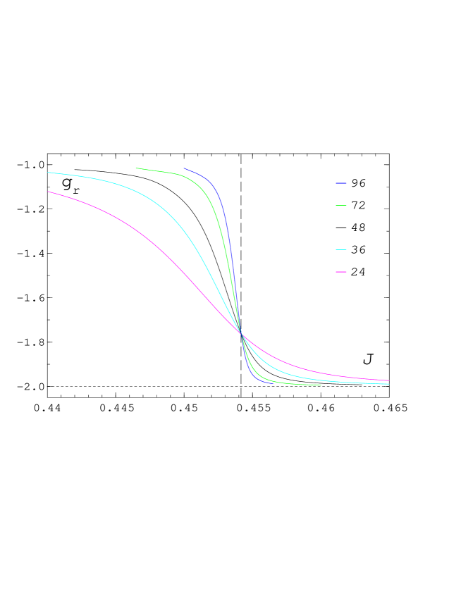
Figure 1: The Binder cumulant $g_{r}$ from Eq. (9) as a function of the coupling $J$. The curves were obtained by reweighting the data. With increasing lattice size $L=24,36,48,72$ and 96, the slope of the respective curve increases close to the critical point. The vertical dashed line denotes $J_{c}$ of Ref. [16].

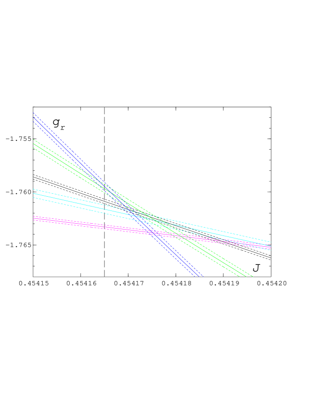
Figure 2: The Binder cumulant $g_{r}$ in the close neighbourhood of the critical point. The figure is an enlargement of Fig. 1. The dashed lines accompanying the solid lines show the jackknife error corridor.

of data in the neighbourhood of the critical point it was natural to verify first the rather precise result of Ballesteros et al. [16]. We have done this by studying the Binder cumulant $g_{r}$, which is directly a finite-size-scaling function

$$g_{r}\;=\;Q_{g}(tL^{1/\nu},L^{-\omega})~{}.$$ (33)

The function $Q_{g}$ depends on the thermal scaling field and on possible irrelevant scaling fields. Here we have specified only the leading irrelevant scaling field proportional to $L^{-\omega}$, with $\omega>0$. At the critical point, $t=0$, $g_{r}$ should therefore be independent of $L$ apart from corrections due to these irrelevant scaling fields. In Fig. 1 we show our results for $g_{r}$ as obtained by reweighting the direct data. We observe, at least on the scale of Fig. 1, no deviation from the scaling hypothesis. However, after a blow-up of the close vicinity of the critical point, as shown in Fig. 2, we can see that the intersection points between curves from different lattices are not coinciding. The shift $\Delta J$ of the crossing point from the infinite volume critical coupling $J_{c}$ can be estimated by expanding the scaling function $Q_{g}$ to lowest order in both variables. For two lattices with sizes $L$ and $L^{\prime}=bL$ one gets

$$\Delta J^{L,L^{\prime}}\;\propto\;s(L,b)\;=\;{1-b^{-\omega}\over b^{1/\nu}-1}L^{-\omega-1/\nu}~{}.$$ (34)

In Fig. 3 we have plotted the $J$-values of the intersection points for each pair of lattices as a function of the variable $s(L,b)$ of Eq. (34). For $\omega$ we used the value 0.79(2) of Ref. [12],

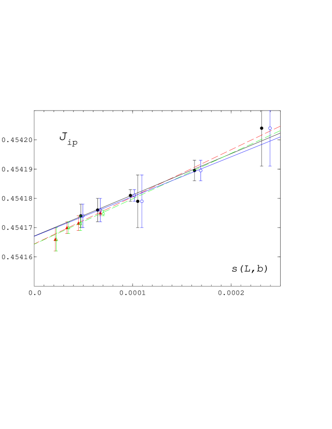
Figure 3: The coupling $J_{ip}$ at the intersection point of $g_{r}(L)$ and $g_{r}(bL)$ for various combinations of $L$ and $b$ as a function of $s(L,b)$, Eq. (34). The filled (empty) symbols were calculated with $\nu=0.669~{}(0.673)$. The dashed (solid) lines are linear fits with (without) the $L=96$ intersection points, denoted here by triangles.

and for $\nu$ we have chosen the two values $\nu=0.669$ and $0.673\>$ as bounds of the probable $\nu$-range. Of course, the intersection points are completely independent of $\nu$ and $\omega$. Only the variable $s(L,b)$ is changing when the exponents are changed. As can be seen in Fig. 3 also the extrapolation to the critical point $J_{c}$ for $L\rightarrow 0$ (or $s(L,b)\rightarrow 0$) is unaffected by the choice of $\nu$. The same applies to a variation of $\omega$. Since the slope of $g_{r}(L=96)$ close to the critical point is rather large, a small numerical uncertainty might shift the intersection points with the other curves considerably. We have therefore determined $J_{c}$ also by fits excluding the results from the largest lattice. Thus we arrive at the final estimate

$$J_{c}\;=\;0.454167(4),$$ (35)

in full agreement with the result $J_{c}=0.454165(4)$ of Ballesteros et al. [16]. In order to be consistent with our previous papers we use in the following again the value of Ref. [16].

In a similar manner one can determine from the same data the universal value $g_{r}(J_{c})$. The difference of the $g_{r}$-values at the intersection points to $g_{r}(J_{c})$ is here

$$\Delta g_{r}^{L,L^{\prime}}\;\propto\;s_{o}(L,b)\;=\;{b^{1/\nu}-b^{-\omega}\over b^{1/\nu}-1}L^{-\omega}~{}.$$ (36)

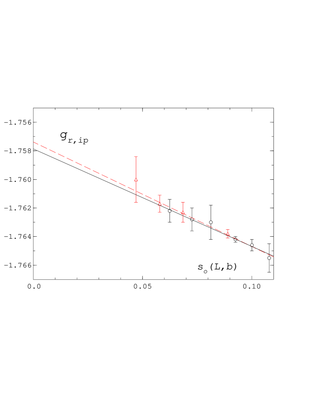
Figure 4: The Binder cumulant $g_{r,ip}$ at the intersection point for various combinations of $L$ and $b$ as a function of $s_{o}(L,b)$, Eq. (36). The dashed (solid) lines are linear fits with (without) the $L=96$ intersection points, denoted here by triangles.

In Fig. 4 we show the extrapolation of $g_{r}$ to the critical point value at $s_{o}(L,b)=0$. A variation of $\omega$ in the range 0.77-0.81 leads only to a shift of $10^{-4}$. The new variable $s_{o}(L,b)$ is practically independent of $\nu$, the influence of $\nu$ is not visible in Fig. 4. Comparing again extrapolations with and without the $L=96$ points one obtains

$$g_{r}(J_{c})\;=\;-1.758(2)~{},\quad{\rm or}\quad{\langle\>(\vec{\phi}^{2})^{2}\,\rangle\over\langle\>\vec{\phi}^{2}\>\rangle^{2}}(J_{c})\;=\;1.242(2)~{},$$ (37)

well in accord with the result of Ref. [11] (see also the long discussion in Ref. [17]).

3.2 The Correlation Length

In our $H=0$ simulations we have measured the correlation length using the second moment formula, Eq. (14). The finite-size-scaling equation for $\xi$ is

$$\xi\;=\;LQ_{\xi}(tL^{1/\nu},L^{-\omega})~{},$$ (38)

and $\xi/L=Q_{\xi}$ is a scaling function like $g_{r}$, that is its value at the critical point is universal for $L\rightarrow\infty$. In Fig. 5 we have plotted our correlation length data divided by $L$. Here formula (14) has also been evaluated for $J>J_{c}$ or $T<T_{c}$ though in this region the data cannot be identified with the correlation length. We see again that all curves intersect at the previously determined

Figure 5: The correlation length $\xi$ divided by $L$ versus $J$ for $L=24,36,48,72$ and 96. The solid lines were calculated by reweighting the data. The dashed vertical line gives the postion of $J_{c}$, the horizontal one the universal value, Eq. (39).

critical point. A closer look into the neighbourhood of $J_{c}$ reveals however similar corrections to scaling as in the case of $g_{r}$. The corresponding extrapolation of the variable $s_{o}(L,b)$ to zero leads for $\xi/L$ to

$$\xi/L\>(J_{c})\;=\;0.593(2)~{}.$$ (39)

This result confirms nicely the value $\xi/L=0.5927$ from the preliminary simulations mentioned in Ref. [12].

Our data for the correlation length can also be used to find the critical amplitude $\xi^{+}$ of Eq. (20). To this end we use a method described in detail in Ref. [18]. We briefly repeat the main arguments assuming for simplicity that there are no corrections to scaling. An observable $O$ with critical behaviour approaches for either positive or negative $t$ and $L\rightarrow\infty$ the limiting form

$$O_{\infty}\;=\;a_{0}|t|^{-\rho}~{},\quad{\rm for~{}}|t|\rightarrow 0~{},$$ (40)

where $a_{0}$ is the critical amplitude and $\rho$ the critical exponent. At finite $L$ the observable satisfies a scaling relation

$$O(t,L)\;=\;L^{\rho/\nu}Q_{O}(x_{t})~{},\quad{\rm with~{}}x_{t}\,=\,tL^{1/\nu}~{}.$$ (41)

Here, $Q_{O}$ is the finite-size-scaling function of $O$. In order to ensure the correct thermodynamic limit for fixed small $|t|$ we must have the relation

$$O_{\infty}\;=\;|t|^{-\rho}\lim_{x_{t}\to\pm\infty}|x_{t}|^{\rho}Q_{O}(x_{t})~{}.$$ (42)

The sign of $x_{t}$ is of course the same as that of $t$. It is clear then, that the function

$$A_{O}(x_{t})\;=\;|x_{t}|^{\rho}Q_{O}(x_{t})~{},$$ (43)

will converge asymptotically to the critical amplitude $a_{0}$. Moreover, $a_{0}$ will be an extreme value of $A_{O}(x_{t})$.

We have applied this method to the correlation length results. In Fig. 6 we show $A_{\xi}(x_{t})$ for the exponent $\nu=0.671$ and various $L$-values. We notice that already at $x_{t}\approx 4$ a plateau is reached and essentially no corrections to scaling are visible. The marginal spread of the data in the plateau region leads only to a small error for the amplitude $\xi^{+}$. Since the scaling variable $x_{t}$ changes with $\nu$ there is however a $\nu$-dependence, which can also be expressed as a dependence on $\alpha$, because of the hyperscaling relation $2-\alpha=d\nu$. In fact, after evaluating $A_{\xi}$ for several $\nu$-values, we find that $\xi^{+}$ is rather exactly a linear function of the used $\alpha$

$$\xi^{+}\;=\;0.4957(20)+0.67(12)~{}\alpha~{}.$$ (44)

This can be seen in Fig. 7, where we compare the fit, Eq. 44, to some directly determined $\xi^{+}$-values.

Figure 6: The amplitude function $A_{\xi}$, Eq. (43), of the correlation length versus the scaling variable $x_{t}$ for $\nu=0.671$ and $L=24,36,48,72$ and 96. The horizontal line indicates the $\xi^{+}$-value.

Figure 7: The critical amplitude $\xi^{+}$, Eq. (20), of the correlation length versus $-\alpha$. The data (circles) are determined from the amplitude function $A_{\xi}(x_{t})$, the solid line is the linear fit (44).

3.3 Specific Heat and Energy Density at $T_{c}$

As mentioned already in Section 2 both the energy density and the specific heat contain additional non-singular terms. This fact complicates of course the determination of the critical amplitudes. We can however calculate the non-singular terms beforehand by a finite-size-scaling analysis directly at the critical point. For that purpose we have made further Monte Carlo runs at $T_{c}$ on 23 lattices with $L=8$ to $L=160$. In these runs we took between 500,000 and $200,000$ measurements each for $L=8-64$ and on the larger lattices between 120,000 and 50,000. The data for the energy density and the specific heat are shown in Fig. 8 as a function of $L$ up to $L=120$. If one expands the scaling functions for $\epsilon$ and $C$ at $T_{c}$ in powers of $L^{-\omega}$ one obtains

$$\epsilon(L) \!\!=\!\! \epsilon_{ns}\>+q_{0\epsilon}L^{(\alpha-1)/\nu}\left(1+q_{1\epsilon}L^{-\omega}+\dots\right)~{},$$ (45)

$$C(L) \!\!=\!\! C_{ns}+q_{0C}L^{\alpha/\nu}\left(1+q_{1C}L^{-\omega}+\dots\right)~{}.$$ (46)

We have fitted the first terms (up to $q_{1}$) of these expansions to the data. In the case of the energy density we find no corrections to scaling, that is $q_{1\epsilon}\approx 0$, and only small corrections for the specific heat. Fits with different $\nu$-values cannot be distinguished in Fig. 8. When we treat $\nu$ as a free fit parameter we get $\nu=0.671(2)$. The quantity $\epsilon_{ns}$ exhibits no noticeable dependency on $\nu$ or $\alpha$ and $\omega$. We find

$$\epsilon_{ns}\;=\;-0.98841(3)~{}.$$ (47)

Figure 8: The energy density (a) and the specific heat (b) versus $L$ at the critical point. The dashed line shows $\epsilon_{ns}$ and the solid lines fits to Eqs. (45) and (46) for $\nu=0.671$ and $\omega=0.79$.

The situation is quite different in the case of the specific heat. Its non-singular part varies from about 50 for $\nu=0.669$ to 16 at $\nu=0.675$. The reason for this strong variation is that the exponent $\alpha=2-3\nu$ is close to zero, when $\nu$ approaches 2/3. Then the background term $C_{ns}$ develops a pole ($\sim 1/\alpha$) which cancels a corresponding pole in the critical amplitude in such a way that the characteristic critical power behaviour ($\sim|t|^{-\alpha}$) turns over into a logarithmic behaviour ($\sim\ln|t|$).

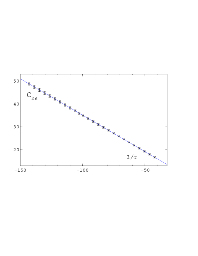
Figure 9: The non-singular part $C_{ns}$ of the specific heat versus $1/\alpha$ from fits to Eq. (46) (stars) with $\omega=0.79$. The solid line is from Eq. (54).

This mechanism for the emergence of the logarithmic singularity as $\alpha\to 0$ is well-known (see Refs. [15] and [19, 20]). We demonstrate it by assuming that

$$C_{ns}(\alpha) \!\!=\!\! c_{ns}^{0}+{c_{ns}^{p}\over\alpha}~{},$$ (48)

$$A^{\pm}(\alpha) \!\!=\!\! a_{0}^{\pm}+a_{1}^{\pm}\alpha+O(\alpha^{2})~{}.$$ (49)

If we insert these equations into Eq. (22) and expand $|t|^{-\alpha}$ for small $\alpha$ we obtain

$$C \!\!=\!\! c_{ns}^{0}+{c_{ns}^{p}\over\alpha}+\left({a_{0}^{\pm}\over\alpha}+a_{1}^{\pm}+O(\alpha)\right)\left(1-\alpha\ln|t|+\dots\right)$$ (50)

$$\!\!=\!\! c_{ns}^{0}+{c_{ns}^{p}+a_{0}^{\pm}\over\alpha}+a_{1}^{\pm}-a_{0}^{\pm}\ln|t|+O(\alpha)~{}.$$ (51)

Evidently the limit of $C$ for $\alpha\to 0$ exists and has a logarithmic $|t|$-dependence, if the pole term vanishes, which requires [19]

$$c_{ns}^{p}\;=\;-a_{0}^{\pm},\quad{\rm and}\quad a_{0}^{+}\;=\;a_{0}^{-}~{}.$$ (52)

The ratio $A^{+}/A^{-}$ is therefore close to 1

$$A^{+}/A^{-}\;=\;1+O(\alpha)~{}.$$ (53)

In Fig. 9 we show the non-singular part $C_{ns}$ of the specific heat resulting from fits to Eq. (46) with $\omega=0.79$ and various values for $\alpha$ plotted versus $1/\alpha$. The $\chi^{2}$ per degree of freedom in each fit is 0.83(1), preferring no particular $\alpha$-value. We see that indeed $C_{ns}$ is linearly dependent on $1/\alpha$. A fit to the ansatz, Eq. (48), gives

$$C_{ns}\;=\;3.35(4)-{0.3175(5)\over\alpha}~{},$$ (54)

with an extremely small $\chi^{2}/N_{f}$ of the order of $10^{-4}$. We conclude from this fact, that the pole term behaviour of $C_{ns}$ is not a numerical accident, but underlines the previous considerations. In order to study the influence of the correction exponent $\omega$ we have repeated the whole analysis of $C(L)$ for the values $\omega=0.77$ and $\omega=0.81$, that is a standard deviation away from the central value 0.79. The $\chi^{2}/N_{f}$ for each single fit to Eq. (46) is again 0.83(1), the new values for $C_{ns}$ coincide within error bars with the values for $\omega=0.79$, however the resultant linear fits in $1/\alpha$ to Eq. (48) at fixed $\omega$, lead to slight changes (again with a $\chi^{2}/N_{f}$ of the order of $10^{-4}$)

$$C_{ns}=\Biggl{\{}\matrix{3.37(4)-0.3165(5)/\alpha&{\rm for}&\omega=0.77\cr 3.33(4)-0.3184(5)/\alpha&{\rm for}&\omega=0.81\cr}~{}~{},$$ (55)

mainly for the pole term parameter $c_{ns}^{p}$.

In the following we shall use the results for $C_{ns}$ to analyze as well the specific heat data for $T\neq T_{c}$. If not explicitly mentioned, the fit results have always been obtained for fixed $\omega=0.79$. We have repeated the following analysis also for $\omega=0.77$ and 0.81 and shall comment on any noticeable changes due to $\omega$.

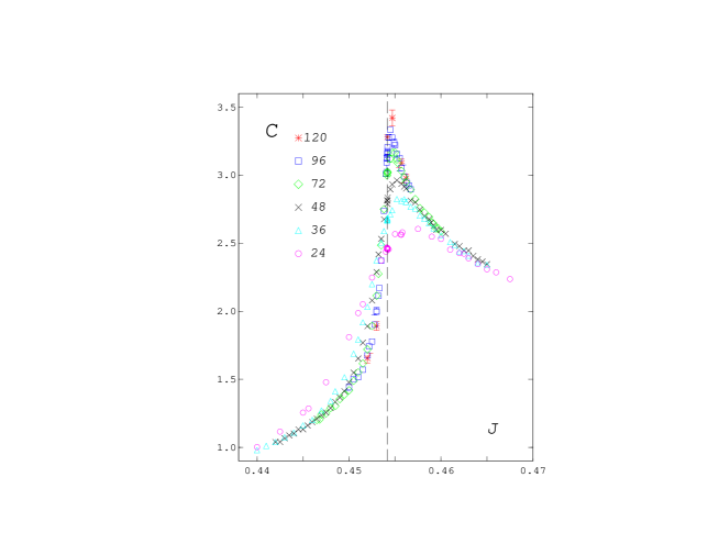
Figure 10: The specific heat data for different $L$ versus the coupling $J$. The dashed line indicates the position of the critical point.

3.4 The Specific Heat and $A^{+}/A^{-}$

In Fig. 10 we have collected all our specific heat data at zero magnetic field for the $L$-values of Table 1. We observe with increasing $L$ a more and more pronounced peak close to $J_{c}$. As already discussed in the introduction, we nevertheless expect a finite peak height even in the thermodynamic limit, since the singular part of $C$ vanishes at the critical point for negative $\alpha$. The peak (and not dip) behaviour implies also that the amplitude $A^{\pm}/\alpha$ must be negative, or that $A^{\pm}$ is positive. The previous analysis of the non-singular contribution to $C$ confirms this consideration: because $c_{ns}^{p}$ is negative we have a positive value $a_{0}^{\pm}=a_{0}$ for the leading part of $A^{\pm}$.

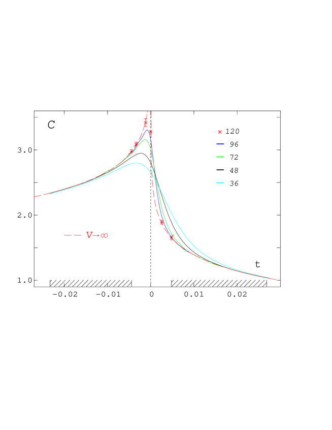
Figure 11: The specific heat versus the reduced temperature $t$ for $L=36,$ 48, 72, 96 and 120 (stars). The solid lines were calculated by reweighting the data, the peak height increases with $L$. The line of long dashes is the fit from the ansatz, Eq. (56), for $\alpha=-0.013$ and $\omega=0.79$. The hatched areas show the fit regions.

We have interpolated the data points by reweighting, apart from the $L=120$ results. The respective curves are plotted in Fig. 11 as a function of $t$. Compared to Fig. 10 we have therefore an exchange of the high ($t>0,J<0)$ and low temperature ($t<0,J>0)$ parts in the figures. In order to find the amplitudes $A^{\pm}$ we have made the following ansatz including correction-to-scaling terms

$$C\;=\;C_{ns}+{A^{\pm}\over\alpha}|t|^{-\alpha}\left(1+c_{1}^{\pm}|t|^{\omega\nu}+c_{2}^{\pm}t\right)~{}.$$ (56)

For a fit to the form (56) the curves from the largest lattices were used in those $t$-ranges, which appear hatched in Fig. 11, that is for $-0.0233\leq t\leq-0.0045$ and $0.0048\leq t\leq 0.0268$. The non-singular part from Eq. (54) was then taken as an input to the fit, whereas the $L=120$ data points served only as a check of the fit result. As an example we show in Fig. 11 the fit for $\alpha=-0.013$. Fits with other small, negative $\alpha$-values work as well and have the same $\chi^{2}$ per degree of freedom, namely $1.03\;$. In Table 2 we present details of the fits for several $\alpha$-values. The two correction-to-scaling contributions are always opposite in sign and cancel therefore to some extent, especially in the high temperature region. The amplitudes $A^{\pm}$ are still $\alpha$-dependent, though in our notation we have taken the anticipated pole behaviour already into account. We find that $A^{+}$ and $A^{-}$ are nearly linear functions of $\alpha$. The $\alpha$-dependence of the fit results for the amplitudes is shown in Fig. 12.

$\alpha$	$A^{+}$	$c_{1}^{+}$	$c_{2}^{+}$	$A^{-}$	$c_{1}^{-}$	$c_{2}^{-}$
-0.007	0.3416(4)	0.020(1)	-0.041(1)	0.3317(4)	0.048(1)	0.086(1)
-0.013	0.3636(6)	0.022(1)	-0.049(2)	0.3445(6)	0.085(1)	0.161(2)
-0.017	0.3790(8)	0.015(1)	-0.041(3)	0.3533(8)	0.109(2)	0.211(4)
-0.019	0.3870(9)	0.010(2)	-0.033(4)	0.3578(9)	0.120(2)	0.237(5)
-0.025	0.4117(13)	-0.016(3)	0.006(6)	0.3718(13)	0.151(4)	0.312(9)

Table 2: The parameters of the fits to Eq. (56) for $\omega=0.79$ and some selected $\alpha$-values. The errors were obtained by Monte Carlo variation of the parameters of $C_{ns}$ in Eq. (54).

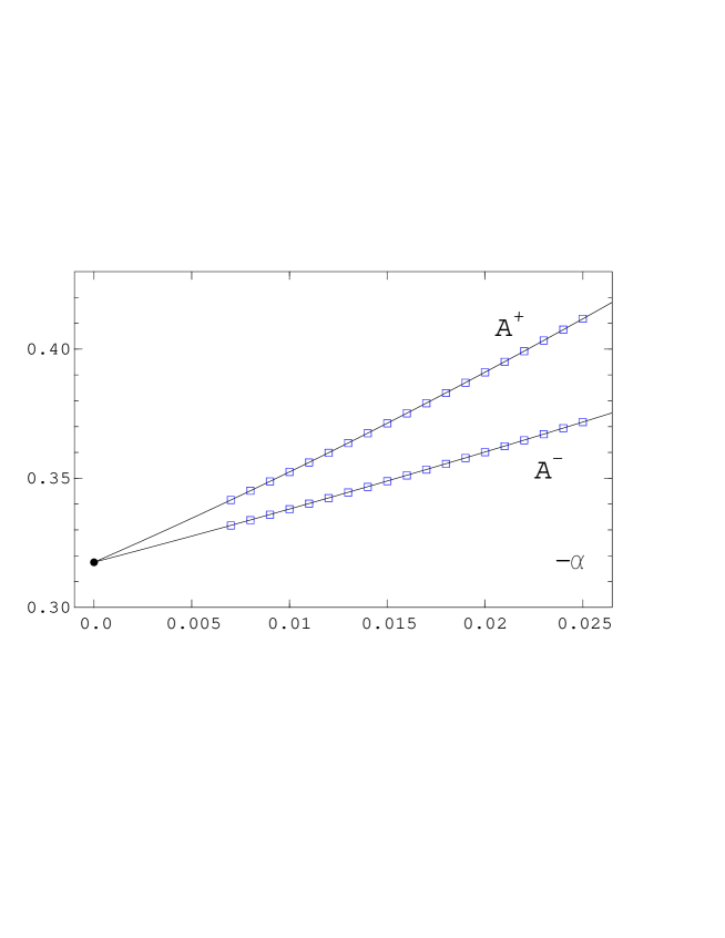
Figure 12: The amplitudes $A^{+}$ and $A^{-}$ versus $-\alpha$ (squares). The filled circle is the value expected from $C_{ns}$; the lines are the parametrizations (58) and (59).

A parametrization of the amplitudes as suggested by Eqs. (49) and (52)

$$A^{\pm}\;=\;a_{0}+a_{1}^{\pm}\alpha+a_{2}^{\pm}\alpha^{2}~{},$$ (57)

works extremely well, as can be seen in Fig. 12, and confirms explicitly the cancellation of the pole terms as predicted in Eq. (52). If $A^{+}$ and $A^{-}$ are independently fitted, that is with perhaps different $a_{0}$, we get $a_{0}^{+}=0.3176(12)$ and $a_{0}^{-}=0.3175(12)$. The final result is found by using Eq. (57) with fixed $a_{0}=0.3175$ (the error in $a_{0}=-c^{p}_{ns}$ is already included in the errors of the $A^{\pm}$-values, which are now parametrized). We obtain

$$A^{+} \!\!= \!\!a_{0}-3.308(36)\alpha+18.4(2.2)\alpha^{2}~{},$$ (58)

$$A^{-} \!\!= \!\!a_{0}-1.975(36)\alpha+\,~{}7.8(2.2)\alpha^{2}~{}.$$ (59)

At this point it is appropriate to discuss the influence of an $\omega$-variation on $A^{+}$ and $A^{-}$. From Eq. (55) we know that a shift in $\omega$ of size $\Delta\omega=0.02$ shifts the pole term parameter $c^{p}_{ns}$ by about $0.3\%$ and therefore we expect a shift of $a_{0}$ by the same amount. In fact that is exactly what happens and it is the only effect, because the new parameters $a_{1}^{\pm}$ and $a_{2}^{\pm}$ coincide inside error bars with the values found for $\omega=0.79$. All in all that results in a common shift of the $A^{+}$ and $A^{-}$-curves in Fig. 12 by again $0.3\%$. As a consequence the universal amplitude ratio $A^{+}/A^{-}$ becomes essentially independent of $\omega$.

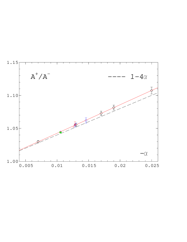
Figure 13: The universal ratio $A^{+}/A^{-}$ versus $-\alpha$. The solid line is obtained from Eqs. (58) and (59), the diamonds by direct calculation from Table 2. The other symbols denote results from the shuttle experiment(square) [7, 8], from Campostrini et al. (circles) [10, 11], from Larin et al. (star) [24] and Kleinert et al. (plus) [25].

The universal ratio $A^{+}/A^{-}$ is sometimes given in terms of a function $\mathcal{P}(\alpha)$ [21]

$$A^{+}/A^{-}\;=\;1-\mathcal{P}\alpha~{}.$$ (60)

Expanding the ratio in powers of $\alpha$ we arrive at the following relation for $\mathcal{P(\alpha)}$

$$\mathcal{P}\;=\;{1\over\alpha}\left(1-{A^{+}\over A^{-}}\right)\;=\;{a_{1}^{-}-a_{1}^{+}\over a_{0}}+\left[{a_{2}^{-}-a_{2}^{+}\over a_{0}}-{a_{1}^{-}\over a_{0}}\cdot{a_{1}^{-}-a_{1}^{+}\over a_{0}}\right]\alpha+\dots~{},$$ (61)

that is, $\mathcal{P}$ goes to a finite limit when $\alpha\to 0$ [21, 22]. In fact, there is a phenomenological relation [9, 23]

$$A^{+}/A^{-}\;=\;1-4\alpha~{},$$ (62)

predicting $\mathcal{P}=4$. Evaluating Eqs. (58) and (59) leads to

$$A^{+}/A^{-}\;=\;1-4.20(5)\alpha+\dots~{},$$ (63)

rather close to the relation (62). In Fig. 13 we show the ratio and compare it to former results from the shuttle experiment [7, 8] as well as some analytical determinations [10, 11] and [24, 25]. We note that our ratio result is in complete accordance with all of the other ratio results. Obviously, they differ among each other simply and solely by assuming different $\alpha$-values. This conclusion was already reached by Campostrini et al. [10], we can however directly confirm it with Eqs. (58) and (59).

4 $A^{+}/A^{-}$ from the Equation of State

The magnetic equation of state describes the critical behaviour of the magnetization in the vicinity of $T_{c}$. As noted by Widom [19] and Griffiths [22] already long ago the equation of state may be integrated to yield the scaling function for the free energy. From subsequent derivatives with respect to the temperature one obtaines then the specific heat and in particular an equation for the universal ratio $A^{+}/A^{-}$. Before we come to this relation we have to briefly discuss the equation of state. The Widom-Griffiths form of the equation of state is given by

$$y=f(x)~{},$$ (64)

where

$$y\equiv h/M^{\delta}~{},\quad x\equiv\bar{t}/M^{1/\beta}~{}.$$ (65)

The variables $\bar{t}$ and $h$ are the normalized reduced temperature and magnetic field

$$\bar{t}=(T-T_{c})/T_{0}~{},\quad h=H/H_{0}~{},$$ (66)

associated with the usual normalization conditions

$$f(0)=1~{},\quad{\rm and}\quad f(-1)=0~{}.$$ (67)

The reduced temperature $\bar{t}$ differs from $t$ by a constant factor ($\bar{t}=[T_{c}/T_{0}]t$), because of the second condition in (67). The normalization constants can be expressed in terms of the critical amplitudes from Eq. (32)

$$T_{0}=B^{-1/\beta}T_{c}=1.18(2)~{},\quad H_{0}=D_{c}=1.11(1)~{}.$$ (68)

The numbers in the last equation have been obtained in Ref. [13] by assuming a special set [12] of critical exponents

$$\beta=0.3490(6)~{},\quad\nu=0.6723(11)~{},$$ (69)

which implies $\alpha\approx-0.017$. The same is true for the equation of state, which was determined numerically in [13] from simulations with a non-zero magnetic field. Using this equation of state will therefore give $A^{+}/A^{-}$ for only that particular value of $\alpha$. Varying $\alpha$ in the range $[-0.0136,-0.0202]$, as suggested by the error of $\nu$, would result in a large variation of $A^{+}/A^{-}$ to begin with (see Fig. 13). Insofar we consider the following calculation mainly as a test of the method.

The results for the equation of state were parametrized in [13] by a combination of a small-$x$ (low temperature) and a large-$x$ (high temperature) ansatz. The small-$x$ form $x_{s}(y)$ was inspired by perturbation theory [26] and incorporates the divergence of the susceptibility on the coexistence line ($x=-1;~{}y=0$) due to the massless Goldstone modes

$$x_{s}(y)+1\;=\;({\widetilde{c}_{1}}\,+\,{\widetilde{d}_{3}})\,y\,+\,{\widetilde{c}_{2}}\,y^{1/2}\,+\,{\widetilde{d}_{2}}\,y^{3/2}\;.$$ (70)

The large-$x$ form $x_{l}(y)$ was derived from Griffiths’s analyticity condition [22]

$$x_{l}(y)\;=\;a\,y^{1/\gamma}\,+\,b\,y^{(1-2\beta)/\gamma}~{}.$$ (71)

The parameter values are

$${\widetilde{c}_{1}}\,+\,{\widetilde{d}_{3}} \!\!=\;~{}0.352(30)~{},\quad~{}{\widetilde{c}_{2}} \!\!=\;~{}~{}0.592(10)~{},$$ (72)

$$a \!\!=\;1.2595(30)~{},\quad b \!\!=\;-1.163(20)~{}.$$ (73)

Because of the normalization $y(0)=1$ we have ${\widetilde{d}_{2}}=1-({\widetilde{c}_{1}}+{\widetilde{d}_{3}}+{\widetilde{c}_{2}})$. The complete equation of state is obtained by interpolation of the low and high temperature parts

$$x(y)\;=\;x_{s}(y)\,\frac{y_{0}^{p}}{y_{0}^{p}+y^{p}}\,+\,x_{l}(y)\,\frac{y^{p}}{y_{0}^{p}+y^{p}}~{},$$ (74)

with $p=6$ and $y_{0}=3.5$.

For negative $\alpha$ the universal ratio $A^{+}/A^{-}$ can be calculated from $f(x)$ using the following formula [27]

$$\frac{A^{+}}{A^{-}}\;=\;\frac{-\int_{0}^{\infty}dx\,x^{\alpha-2}\,[f^{\prime}(0)-f^{\prime}(x)+f^{\prime\prime}(0)x]}{f^{\prime}(0)/(1-\alpha)\,+\,f^{\prime\prime}(0)/\alpha\,+\,\int_{-1}^{0}dx\,(-x)^{\alpha-2}\,[f^{\prime}(0)-f^{\prime}(x)+f^{\prime\prime}(0)x]}\;.$$ (75)

The main contribution to both the nominator and the denominator is $f^{\prime\prime}(0)/\alpha$. A more appropriate representation of $A^{+}/A^{-}$ is therefore

$$\frac{A^{+}}{A^{-}}\;=\;\frac{1+[\alpha/f^{\prime\prime}(0)]\,F_{N}}{1+[\alpha/f^{\prime\prime}(0)]\,F_{D}}~{},$$ (76)

where

$$\!\!\!\!F_{N}\!\! \!\!=\!\! \!\!-{f^{\prime}(0)\over 1-\alpha}-\int_{0}^{1}dx\,x^{\alpha-2}\,[f^{\prime}(0)-f^{\prime}(x)+f^{\prime\prime}(0)x]+\int_{1}^{\infty}dx\,x^{\alpha-2}\,f^{\prime}(x)\,,$$ (77)

$$\!\!\!\!F_{D}\!\! \!\!=\!\! \!\!{f^{\prime}(0)\over 1-\alpha}\,+\,\int^{0}_{-1}dx\,(-x)^{\alpha-2}\,[f^{\prime}(0)-f^{\prime}(x)+f^{\prime\prime}(0)x]\,.$$ (78)

Let us denote the integrals in Eq. (77) by $I_{1}$ and $I_{2}$, the one in Eq. (78) by $I_{3}$. To a good approximation we can calculate the integrals $I_{1}$ and $I_{3}$ as well as the derivatives from the low temperature equation (70). In order to obtain $I_{2}$ we first rewrite the integral as

$$I_{2}\;=\;-f(1)+(2-\alpha)\int^{\infty}_{f(1)}dyy{dx\over dy}x^{\alpha-3}~{},$$ (79)

and evaluate the remaining integral from the interpolation formula (74), using for $f(1)$ the low temperature value 2.4448. For the derivatives we find

$$f^{\prime}(0)\!\! = \!\!2\left(3-{\widetilde{c}_{1}}-{\widetilde{d}_{3}}-2{\widetilde{c}_{2}}\right)^{-1}\;=\;1.366\pm 0.034~{},$$ (80)

$$f^{\prime\prime}(0)\!\! = \!\![f^{\prime}(0)]^{\,3}\left((3/4)({\widetilde{c}_{1}}+{\widetilde{d}_{3}}-1)+{\widetilde{c}_{2}}\right)\;=\;0.270\pm 0.064~{},$$ (81)

and for the integrals

$$I_{1}\;=\;0.203\,\pm 0.02,\quad I_{2}\;=\;1.749\,\pm 0.03,\quad I_{3}\;=\;0.512\,\pm 0.02.$$ (82)

The errors in the integrals were obtained by Monte Carlo variation of the initial parameters in Eqs. (72) and (73). When this procedure is also applied to the complete expression (76) one obtains

$$A^{+}/A^{-}\;=\;1.12\pm 0.05~{}.$$ (83)

The first conclusion to be drawn from this result is that this method is not well suited for the calculation of the ratio, at least with the parametrization of the equation of state of Ref. [13]. Though the result (83) is compatible with our directly determined ratio $A^{+}/A^{-}(\alpha=-0.017)\,=\,1.073(3)$, the error is rather large. The main source of the error is evidently the inaccurate value of $f^{\prime\prime}(0)$. That this quantity plays an important role is of course not unexpected, because $A^{+}$ and $A^{-}$ are the amplitudes of the specific heat, which is again the second derivative of the free energy density. Our parametrization was not devised for that purpose, but for a correct description of the Goldstone effect near to $x=-1$ and the limiting behaviour for $x\to\infty$. That is why it led to a precise determination of $R_{\chi}$ and the constant $c_{f}$

$$R_{\chi}=\lim\limits_{x\to\infty}x^{\gamma}/f(x)\,=\,1.356(4)\,,\quad c_{f}\equiv\lim\limits_{x\to-1}(1+x)^{-2}f(x)\,=\,2.85(7)\,.$$ (84)

Campostrini et al. have used a different representation of the equation of state [28, 11], based on Josephson’s parametrization [29] of $M,\bar{t}$ and $H$ in terms of the variables $R$ and $\theta$ and parametric functions. In order to fix these functions approximately the authors utilized the results of an analysis of the high-temperature expansion of an improved lattice Hamiltonian. The values obtained for $A^{+}/A^{-}$ compare well with our direct determination and were already shown in Fig. 13. The corresponding equation of state differs however somewhat in the low and medium temperature regions from the data points from our non-zero field simulations [13]. The question arises then whether the same data may be described as well in the schemes introduced by Campostrini et al. . Such alternative fits of the data have been carried out by two of us [30]. The $\chi^{2}$ per degree of freedom of these fits is generally high, in particular for scheme $A$ of Ref. [28]. The fits according to scheme $B$ are considerably better and lead to a ratio $A^{+}/A^{-}=1.070(13)$, again compatible with our direct determination. The simultaneously calculated ratio $R_{C}$ is however much larger (0.165-0.185) than expected from analytical calculations (0.123-0.130) [31, 25]. We therefore do not pursue this method of calculation here in more detail.

5 Simulations with $H>0$

We have performed additional simulations with a positive magnetic field $H$ on the critical line to find the remaining critical amplitudes for the specific heat and the longitudinal and transverse correlation lengths.

$L$	$H$-range	$N_{cu}$	$N_{meas}[1000]$	$N_{H}$	$N_{tot}$
36	0.0007-0.05	50-100	30-40	25	36
48	0.0001-0.03	50-100	30-40	30	39
72	0.0001-0.005	60-300	20	15	23
96	0.0001-0.0015	60-80	12-20	8	16

Table 3: Survey of the new Monte Carlo simulations at $T_{c}$ on different lattices. $N_{cu}$ is the number of cluster updates between the measurements, $N_{meas}$ the number of measurements per $H$-value in units of 1000 and $N_{H}$ the number of $H$-values at which new runs were performed. $N_{tot}$ is the total number of $H$-values where we have data.

The linear extensions of the lattices we used were $L=36,48,72$ and 96. These measurements were combined with those from Ref. [13] to cover the $H$-range appropriately. Some of the new data have already been used in Ref. [32]. In Table 3 we give more details of these simulations.

5.1 The Specific Heat on the Critical Line

In Fig. 14 we show our specific heat data as a function of the magnetic field $H$. Since there are no noticeable systematic finite size effects we can use these data to fit them to the ansatz

$$C\;=\;C_{ns}+{A_{c}\over\alpha_{c}}H^{-\alpha_{c}}(1+c_{h}H^{\omega\nu_{c}})~{}.$$ (85)

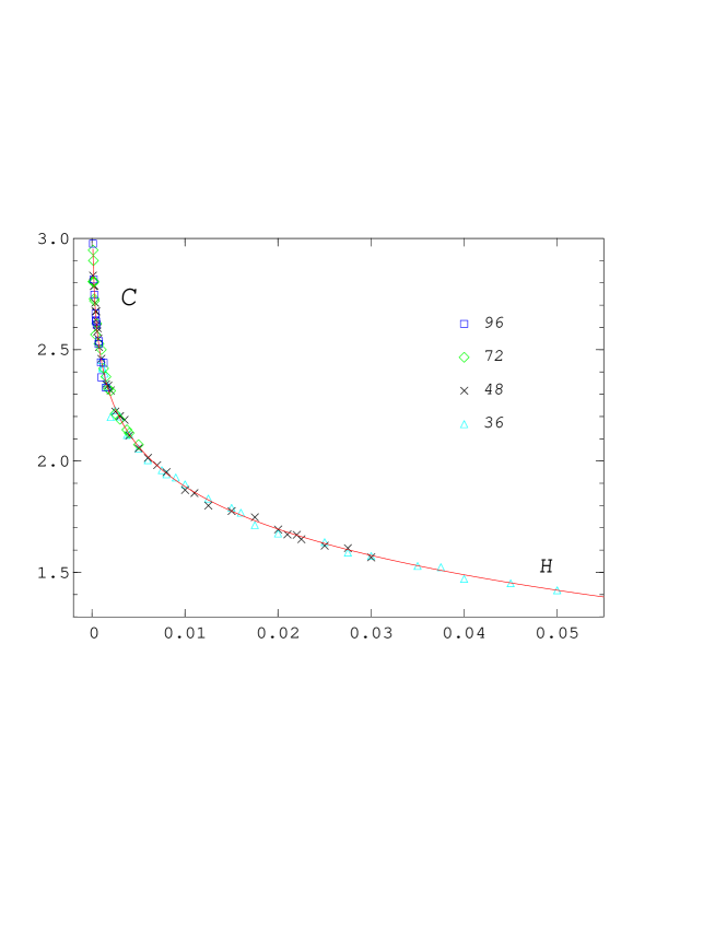
Figure 14: The specific heat at $T_{c}$ for $L=36,48,72$ and 96 as a function of $H$. The line is the fit (85) for $\alpha_{c}=-0.0078\,(\nu=0.671)$ and $\omega=0.79$.

Here, $C_{ns}$ is the same non-singular term, which we have already determined in Section 3.3 as a function of $\alpha$ (or $\nu$) with the result (54). Because of the dependence of $C$ on $\alpha_{c}$ and $\nu_{c}$ the amplitudes $A_{c}$ and $c_{h}$ depend on two critical exponents. The second exponent will however not introduce a sizeable variation in the amplitudes. We therefore treat the exponent $\beta$ as fixed to the value $\beta=0.349\,$, in accord with our previous calculations. With the relations

$$\beta\delta\;=\;2-\beta-\alpha~{},\quad\alpha_{c}\;=\;{\alpha\over 2-\beta-\alpha}~{},\quad\alpha\;=\;{\alpha_{c}(2-\beta)\over 1+\alpha_{c}}~{},$$ (86)

the linear dependence of $C_{ns}$ on $1/\alpha$ can be rewritten as one on $1/\alpha_{c}$

$$C_{ns} = c_{ns}^{0}+{c_{ns}^{p}\over 2-\beta}\left(1+{1\over\alpha_{c}}\right)\vspace*{0.2cm}$$ (87)

$$= 3.16(4)-{0.1923(3)\over\alpha_{c}}~{}.$$ (88)

$\alpha_{c}$	$\alpha$	$A_{c}$	$c_{h}$	$\chi^{2}/N_{f}$
-0.00422	-0.007	0.2006(2)	0.0203(1)	1.09
-0.00781	-0.013	0.2080(3)	0.0344(2)	1.09
-0.01019	-0.017	0.2131(5)	0.0423(4)	1.10
-0.01138	-0.019	0.2156(5)	0.0458(4)	1.10
-0.01492	-0.025	0.2235(7)	0.0546(8)	1.11

Table 4: The parameters of the fits to Eq. (85) for some selected $\alpha_{c}$-values at fixed $\beta=0.349$ and $\omega=0.79$. The errors were obtained by Monte Carlo variation of the parameters of $C_{ns}$ in Eq. (88).

We took this form of $C_{ns}$ as an input to the fits of $C$ with Eq. (85). The $H$-range for the fits was $0.0001\leq H\leq 0.05$. We have convinced ourselves that smaller $H$-ranges (up to 0.02 or 0.03) lead inside the error bars to the same results for the amplitudes. In Table 4 we present details of the fits for several $\alpha_{c}$-values, in Fig. 15 we show the amplitude $A_{c}$ as a function of $\alpha_{c}$. As in the case of the amplitudes $A^{\pm}$ the pole of $C_{ns}$ in Eq. (88) is compensated by the corresponding pole term in $A_{c}/\alpha_{c}$. We have therefore parametrized the $\alpha_{c}$-dependence of $A_{c}$ in analogy to Eq. (57) with the fixed value $A_{c}(\alpha_{c}=0)\,=\,0.1923\,$ and find

$$A_{c}\;=\;0.1923-1.919(42)\alpha_{c}+11.6(4.1)\alpha_{c}^{2}~{}.$$ (89)

From Fig. 15 we see that this parametrization describes the data very well. Like in the study of the $\omega$-dependence of $A^{\pm}$ in Section 3.4 we found changes of similar size for the amplitude $A_{c}$ due to a variation of $\omega$. They lead to an additional error of $A_{c}$ of size 0.0006 at $\alpha_{c}=-0.00422$, which decreases to 0.0004 at $\alpha_{c}=-0.01492$.

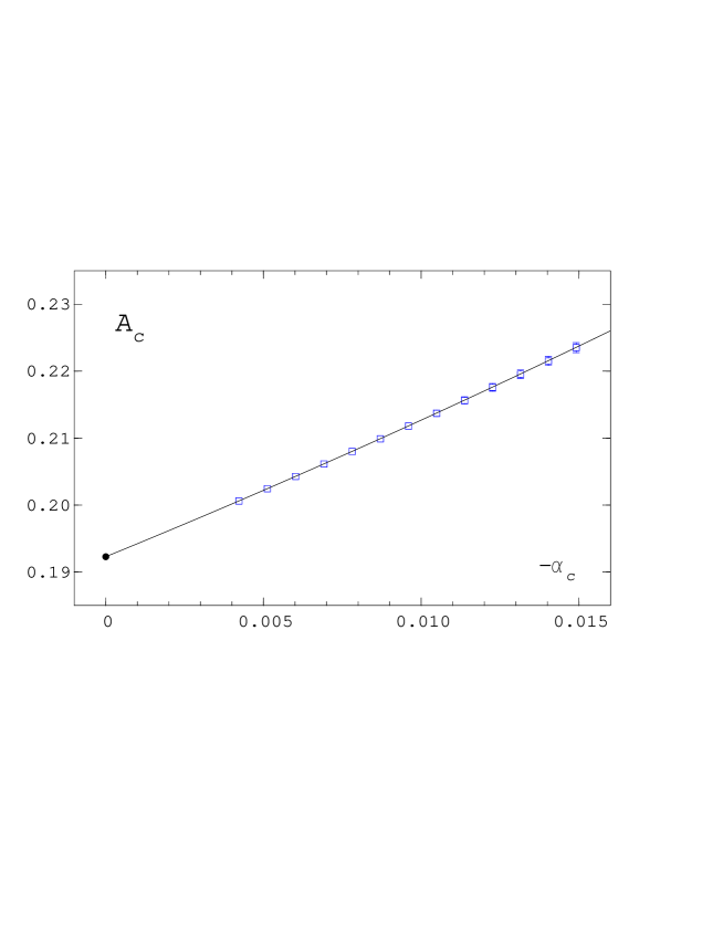
Figure 15: The amplitude $A_{c}$ versus $-\alpha_{c}$ (squares) for $\omega=0.79$. The filled circle shows the value expected from $C_{ns}$, the line is the parametrization (89).

5.2 The Correlation Lengths on the Critical Line

The simulation results for the transverse and longitudinal correlation lengths are shown in Fig. 16 a) and b). For the transverse correlation length $\xi_{T}$ one can hardly detect finite size effects, whereas the longitudinal correlation length $\xi_{L}$ shows more fluctuations and a systematic deviation to higher $\xi_{L}$-values, when one decreases the magnetic field $H$. The smaller the lattice, the earlier this behaviour sets in. In order to determine the amplitudes we have fitted our results to the following form

$$\xi_{T,L}\;=\;\xi_{T,L}^{c}H^{-\nu_{c}}\left(1+c_{T,L}H^{\omega\nu_{c}}\right)~{}.$$ (90)

$\nu_{c}$	$\alpha$	$\xi_{T}^{c}$	$c_{T}$	$\xi_{L}^{c}$	$c_{L}$
0.40350	-0.007	0.6709(14)	0.024(13)	0.3427(15)	-0.258(33)
0.40325	-0.013	0.6724(14)	0.019(14)	0.3435(15)	-0.263(33)
0.40307	-0.017	0.6735(14)	0.015(14)	0.3441(15)	-0.266(33)
0.40299	-0.019	0.6740(14)	0.013(14)	0.3443(15)	-0.268(32)
0.40274	-0.025	0.6755(14)	0.008(14)	0.3451(15)	-0.273(32)

Table 5: The parameters of the fits to Eq. (90) for some selected $\nu_{c}$-values and $\omega=0.79$. The $\chi^{2}/N_{f}$-values varied for $\xi_{T}$ between 0.89 and 0.86, for $\xi_{L}$ it was $0.67$.

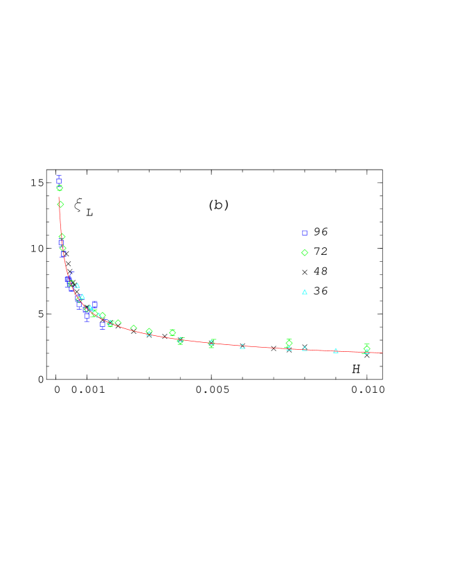
Figure 16: The correlation lengths $\xi_{T}$ (a) and $\xi_{L}$ (b) at $T_{c}$ for $L=36,48,72$ and 96 as a function of $H$. The lines are the fits (90) for $\nu_{c}=0.40325$ and $\omega=0.79\,$.

In the transverse case we used the reweighted data for $L=72$ in the $H$-interval [0.0005,0.0025], for $L=48$ in [0.002,0.02] and for $L=36$ in [0.015,0.03]. From Table 5 we see that the correction term is essentially zero. Correspondingly, there is no $\omega$-dependence and a fit with $c_{T}\equiv 0$ works just as well (even with the same $\chi^{2}/N_{f}$), and leads to a slight increase in the amplitude value, which is of the order of the error given in Table 5. The dependence of the amplitude $\xi_{T}^{c}$ on $\nu_{c}$ or $\alpha$ is linear but the slope is very small. In order to determine the longitudinal amplitude $\xi_{L}^{c}$ we have fitted the reweighted data for $L=72$ in the $H$-interval [0.0005,0.00175] together with those for $L=48$ in [0.00175,0.01]. Here, the correction term is not zero, but the variation due to $\omega$ is still negligible. The $\nu_{c}$- or $\alpha$-dependence is the same as for $\xi_{T}^{c}$, the ratio of the two correlations lengths is a fixed number

$$\xi_{T}^{c}/\xi_{L}^{c}\;=\;1.957(10)~{},$$ (91)

independent of the critical exponents. It is well-known (see Refs. [15] and [33, 34]) that at zero field on the coexistence line $t<0$ the longitudinal correlation function $G_{L}$ is for large distances $|\vec{r}|$ connected to the transverse one by

$$G_{L}(\vec{r},t)\;\approx\;{1\over 2}(N-1)[G_{T}(\vec{r},t)/M]^{2}~{},$$ (92)

where in our case $N=2$. The relation is expected to hold also for small non-zero fields $H$ near the phase boundary in the regime of exponential decay implying a factor 2 between the correlation lengths. It is remarkable, that we find approximately such a value for the ratio at $t=0$. A similar observation has been made for the $3d~{}O(4)$ model [35].

5.3 The Stiffness Constant on the Coexistence Line

The stiffness constant $\rho_{s}(T)$ is related to the helicity modulus $\Upsilon$ [36] by

$$\rho_{s}\;=\;\Upsilon/T~{},$$ (93)

which can be measured in Monte Carlo simulations. This was done e. g. in Refs. [37] and [38]. Here we follow a different strategy, which we applied already in Ref. [13] to find the magnetization on the coexistence line. The $L$ or volume dependence of $M$ at fixed $J$ and fixed small $H$ is described by the $\epsilon$-expansion of chiral perturbation theory (CPT) in terms of two low energy constants. One is the Goldstone-boson-decay constant $F$, the other the magnetization $\Sigma$ of the continuum theory for $H=0$ and $V\rightarrow\infty$. The square of the constant $F$ is proportional to the helicity modulus. In our notation, which is different from the one in CPT (see the remark in the last paragraph of Ref. [39]) we have

$$\Upsilon\;=\;F^{2}/J~{},\quad{\rm implying}\quad\rho_{s}\;=\;F^{2}~{}.$$ (94)

The formulae, which are needed for the fits to determine the constants, are summarized in Ref. [13] and were taken from Ref. [39]. In Table 6 we list the results for the Goldstone-boson-decay constant $F$ at various $J$-values. We performed simulations at $H=0.0001$ on lattices with linear extensions $L=8,10,12,16,20,24,30,36,40,48$ and 56. By construction the $\epsilon$-expansion is only applicable in a range where $m_{\pi}L\raise 1.29167pt\hbox{$<$\kern-7.5pt\raise-4.73611pt\hbox{$\sim$}}1$. This condition translates into the equation

$$H{\Sigma\over\sqrt{J}}\;\raise 1.29167pt\hbox{$<$\kern-7.5pt\raise-4.73611pt\hbox{$\sim$}}\;\left({F\over L}\right)^{2}~{},$$ (95)

$J=1/T$	$F$	$\Delta F$	$L_{min}$	$L_{max}$
0.462	0.1993	0.0096	8,10,12	36,40
0.465	0.2275	0.0060	8,10,12	40,48
0.470	0.2596	0.0050	8,10,12	40,48
0.480	0.3091	0.0018	8,10,12	48
0.500	0.3795	0.0114	8,10,12	48,56
0.525	0.4379	0.0040	8,10,12	48,56
0.550	0.4755	0.0028	8,10,12	56

Table 6: The Goldstone-boson-decay constant $F$ at various $J$-values from fits on data from lattices with $L$ in the range $[L_{min},L_{max}]$.

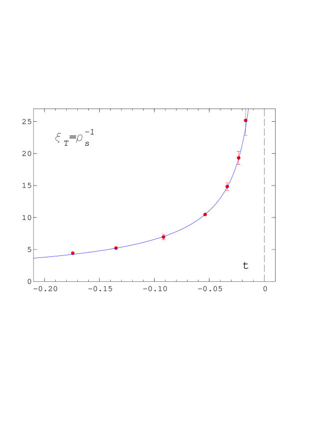
Figure 17: The inverse of the stiffness constant $\rho_{s}^{-1}=\xi_{T}$ on the coexistence line from chiral perturbation theory. The solid line is the fit (96) with $\nu=0.671$ and $\omega=0.79$.

and excludes the use of too large $L$-values. For each $J$ we fitted different sets of data from lattices between $[L_{min},L_{max}]$ and averaged the obtained $F$-values. The errors on $F$ include the variations of these results. If we compare our $F$-values to the corresponding ones of Ref. [39] we find generally somewhat lower numbers. This may be due to the fact that in Ref. [39] data from single lattices instead of sets of data from different lattices were fitted. The transverse correlation length $\xi_{T}$ on the coexistence line is now derived from the inverse of the stiffness constant or $F^{-2}$. It is plotted in Fig. 17. Here, we have not as many and as accurate data as in Fig. 16 a). In order to determine the amplitude $\xi_{T}^{-}$ we fit our data points up to $J=0.525$ to the ansatz

$$\xi_{T}\;=\;\xi_{T}^{-}(-t)^{-\nu}\left(1+c_{T}^{-}(-t)^{\omega\nu}\right)~{}.$$ (96)

Table 7 contains the fit parameters for different $\nu$ or $\alpha$-values. We observe, as for $\xi_{T}^{c}$, a linear dependence of the amplitude $\xi_{T}^{-}$ on $\alpha$ with a very small slope. A change of $\omega$ by 0.02 leads only to a shift in $\xi_{T}^{-}$ of a tenth of the error in Table 7.

$\nu$	$\alpha$	$\xi_{T}^{-}$	$c_{T}^{-}$	$\chi^{2}/N_{f}$
0.6690	-0.007	1.680(52)	-0.55(10)	0.08
0.6710	-0.013	1.665(52)	-0.54(11)	0.08
0.6723	-0.017	1.655(51)	-0.53(11)	0.08
0.6730	-0.019	1.650(51)	-0.53(11)	0.08
0.6750	-0.025	1.636(51)	-0.52(11)	0.07

Table 7: The parameters of the fits to Eq. (96) for several $\nu$-values and $\omega=0.79$.

6 The Universal Amplitude Ratios

After having determined all the amplitudes which appear in Eqs. (27) to (30) we can calculate the corresponding universal ratios. Since the ratio $U_{0}=A^{+}/A^{-}$ has already been discussed in great detail we start with the ratio $U_{\xi}$ of the correlation lengths for $H=0$. From Eq. (44) and Table 7 we find

$$U_{\xi}\;=\;\xi^{+}/\xi^{-}_{T}\;=\;0.293(9)~{},$$ (97)

independent of the used $\alpha$-value. The $\epsilon$-expansion of this ratio was derived by Hohenberg et al. [23] to $O(\epsilon)$ and extended by Bervillier [40] to $O(\epsilon^{2})$ resulting in $U_{\xi}=0.27$ and 0.33, respectively. Okabe and Ideura [41] corrected the expansion of Bervillier (not the numerical value) and computed the ratio in $1/N$-expansion to $U_{\xi}=0.140$. The $\epsilon$-expansion results are comparable in size to our value in (97), the $1/N$-expansion result, however, seems to be too small.

The ratios connecting the specific heat and correlation length amplitudes are related by

$$R_{\xi}^{+}\;=\;R_{\xi}^{T}{U_{0}}^{1/d}U_{\xi}~{},$$ (98)

and they depend on the used $\alpha$, mainly because of the specific heat amplitudes. In Table 8 we have listed the ratios $R_{\xi}^{+}$ and $R_{\xi}^{T}$. From the $\alpha$-expansions (44) and (58) we find

$$R_{\xi}^{+}\;=\;0.3382(14)-0.717(96)\alpha+0.87(1.13)\alpha^{2}~{}.$$ (99)

For $R_{\xi}^{T}$ one can derive a similar formula representing the values of Table 8

$$R_{\xi}^{T}\;=\;1.1580-0.696\alpha+0.97\alpha^{2}\pm 0.036~{}.$$ (100)

There exist several theoretical estimates of $R_{\xi}^{+}$ which compare well with our result: 0.355(3) [$\alpha=-0.0146$] [11] and 0.361(4) [42], both from high-temperature expansions; 0.36 [40] from the $\epsilon$-expansion, and 0.3597(10) [43] and 0.3606(20) [44] from $3d$ field theory. Apart from the first result, we could not relate a definite $\alpha$-value to the respective estimate. The ratio $R_{\xi}^{T}$ was calculated from the $\epsilon$-expansion [23, 40] with the result 1.0(2) [15], well in accord with our value.

$\nu$	$\alpha$	$R_{\xi}^{+}$	$R_{\xi}^{T}$	$R_{C}$	$R_{A}$	$Q_{2}^{T}$
0.6690	-0.007	0.3432(15)	1.163(36)	0.118(4)	0.0515(17)	0.834(21)
0.6710	-0.013	0.3476(18)	1.167(36)	0.125(4)	0.0534(18)	0.849(21)
0.6723	-0.017	0.3505(21)	1.170(36)	0.130(4)	0.0547(18)	0.860(21)
0.6730	-0.019	0.3520(22)	1.171(36)	0.133(5)	0.0554(19)	0.865(21)
0.6750	-0.025	0.3563(27)	1.176(36)	0.142(5)	0.0574(19)	0.881(22)

Table 8: The universal ratios from Eqs. (28), (29) and (30) as a function of the used exponents $\nu$ and $\alpha$.

The remaining universal ratios $R_{\chi},R_{C},R_{A}$ and $Q_{2}^{T}$ are all dependent on the amplitude $C^{+}$ of the susceptibility and/or the amplitudes $B$ and $d_{c}(D_{c})$ of the magnetization. We mentioned already that we had determined $R_{\chi},B$ and $d_{c}$ in Ref. [13], although for fixed $\nu=0.6723$. In the following we proceed as in Section 5.1, that is we keep $\beta$ fixed to 0.349 and assume in addition that the $\nu$-dependencies of $R_{\chi},B$ and $d_{c}$ are negligible. In Table 8 we present the ratios $R_{C}$ and $Q_{2}^{T}$ as calculated from

$$R_{C}\;=\;A^{+}R_{\chi}D_{c}^{-1}B^{-1-\delta}~{},\quad Q_{2}^{T}\;=\;(\xi^{c}_{T}/\xi^{+})^{\gamma/\nu}R_{\chi}(d_{c}/B)^{\delta-1}/(1+1/\delta)~{},$$ (101)

and $R_{A}$ directly from the definition in Eq. (30), using our newly determined amplitudes $A^{+},A_{c},\xi^{c}_{T}$ and $\xi^{+}$. We could not find any previous results for $R_{A}$ and $Q_{2}^{T}$ in the literature, however, the ratio $R_{C}$ has been calculated theoretically in several ways. From Table 8 we see that $R_{C}$ is increasing with decreasing $\alpha$, which is due to the factor $A^{+}$. In comparing our values to the analytical results we quote therefore the used $\alpha$-values. The ratio $R_{C}$ calculated from $3d$ field theory in Ref. [31] is 0.123(3) [$\alpha=-0.01285$], in Ref. [25] 0.12428 [$\alpha\!=\!-0.01056$]; from the high-temperature expansion in Ref. [11] one finds 0.127(6) [$\alpha=-0.0146$]. The results are in full agreement with our calculation, though that of Ref. [25] is somewhat higher than the other ones. The old $\epsilon$-expansion result 0.103 of Aharony and Hohenberg [45] seems to be too small.

7 Conclusions

We have calculated the major universal amplitude ratios of the three-dimensional $O(2)$ model from Monte Carlo simulations. To reach this goal a large amount of computer time had to be spent on the cluster of alpha-workstations of the department of physics at the University of Bielefeld. Most of the computer time went into the production of reliable specific heat data for the direct determination of $A^{+}/A^{-}$. Initially we had hoped to improve the accuracy of the exponent $\alpha$ (or $\nu$) from these data. As it turned out, however, the specific heat data could be fitted to a whole range of $\alpha$-values with the same $\chi^{2}/N_{f}$, extending even to $\alpha=0$. This raises the question, whether the experimental shuttle data are really fixing the $\alpha$-value to exactly -0.01056, the same value as in $3d$ field theory expansions [1]. The positive aspect of the indifference of the fits to the specific heat data to $\alpha$-variations was that we could study the numerical changes induced by these variations in the universal ratio $A^{+}/A^{-}$ and the background term $C_{ns}$. As a result we were able to confirm the conjectured pole (in $1/\alpha$) behaviour of the amplitudes and the background term and the mutual cancellation of the pole contributions. The same pole behaviour was observed for the specific heat amplitude on the critical line. The functional dependence of $A^{+}/A^{-}$ on the used $\alpha$-value is in complete accordance with all other ratio results and not far from the phenomenological relation $A^{+}/A^{-}=1-4\alpha$. We have also determined $A^{+}/A^{-}$ from the numerical equation of state, but we think the method relies too much on the chosen parametrization.

In order to find the amplitude of the transverse correlation length on the coexistence line we used chiral perturbation theory. This enabled us to calculate the less known ratios $R_{\xi}^{T}$ and $U_{\xi}$. The latter is independent of the used $\alpha$, like the ratio $\xi_{T}^{c}/\xi_{L}^{c}$ on the critical line, which is remarkably close to 2 - a prediction expected for $T<T_{c}$ from the correlation functions close to the phase boundary. Our results for $R_{\xi}^{+}$ and $R_{C}$ are in full agreement with the best theoretical estimates; $R_{A}$ and $Q_{2}^{T}$ are new and remain untested for the moment. Acknowledgements

We are grateful to Jean Zinn-Justin, Michele Caselle, Martin Hasenbusch and Andrea Pelissetto for discussions and to Ettore Vicari for his comments on the calculation of $A^{+}/A^{-}$ from the equation of state. Our work was supported by the Deutsche Forschungsgemeinschaft under Grant No. FOR 339/1-2, the work of A. C. and T. M. in addition by FAPESP, Brazil (Project No. 00/05047-5).

References

- [1] J. Zinn-Justin, Phys. Rept. 344 (2001) 159 [hep-th/0002136].
- [2] J. C. Le Guillou and J. Zinn-Justin, Phys. Rev. Lett. 39 (1977) 95.
- [3] J. C. Le Guillou and J. Zinn-Justin, Phys. Rev. B 21 (1980) 3976.
- [4] R. Guida and J. Zinn-Justin, J. Phys. A 31 (1998) 8103 [cond-mat/9803240].
- [5] W. M. Fairbank, M. J. Buckingham and C. F. Kellers, Proceedings of the Fifth International Conference on Low Temp. Phys., Madison, WI, 1957, p.50.
- [6] M. I. Bagatskii, A. V. Voronel’ and V. G. Gusak, Sov. Phys. JETP 16 (1963) 517.
- [7] J. A. Lipa, D. R. Swanson, J. A. Nissen, T. C. P. Chui and U. E. Israelsson, Phys. Rev. Lett. 76 (1996) 944.
- [8] J. A. Lipa, D. R. Swanson, J. A. Nissen, Z. K. Geng, P. R. Williamson, D. A. Stricker, T. C. P. Chui, U. E. Israelsson and M. Larson, Phys. Rev. Lett. 84 (2000) 4894.
- [9] A. Pelissetto and E. Vicari, cond-mat/0012164, to appear in Phys. Rept. .
- [10] M. Campostrini, M. Hasenbusch, A. Pelissetto, P. Rossi and E. Vicari, Nucl. Phys. Proc. Suppl. 94 (2001) 857 [hep-lat/0010041].
- [11] M. Campostrini, M. Hasenbusch, A. Pelissetto, P. Rossi and E. Vicari, Phys. Rev. B 63 (2001) 214503 [cond-mat/0010360].
- [12] M. Hasenbusch and T. Török, J. Phys. A32 (1999) 6361 [cond-mat/9904408].
- [13] J. Engels, S. Holtmann, T. Mendes and T. Schulze, Phys. Lett. B 492 (2000) 219 [hep-lat/0006023].
- [14] A. L. Talapov and H. W. Blöte, J. Phys. A29 (1996) 5727 [cond-mat/9603013].
- [15] V. Privman, P. C. Hohenberg and A. Aharony, in Phase Transitions and Critical Phenomena, vol. 14, edited by C. Domb and J. L. Lebowitz (Academic Press, New York, 1991).
- [16] H. G. Ballesteros, L. A. Fernández, V. Martín-Mayor and A. Muñoz Sudupe, Phys. Lett. B 387 (1996) 125 [cond-mat/9606203].
- [17] P. Arnold and G. D. Moore, Phys. Rev. E64 (2001) 066113 [cond-mat/0103227].
- [18] J. Engels and T. Scheideler, Nucl. Phys. B 539 (1999) 557 [hep-lat/9808057].
- [19] B. Widom, J. Chem. Phys. 43 (1965) 3898.
- [20] F. J. Wegner, Phys. Rev. B 5 (1972) 4529.
- [21] M. Barmatz, P. C. Hohenberg and A. Kornblit, Phys. Rev. B 12 (1975) 1947.
- [22] R. B. Griffiths, Phys. Rev. 158 (1967) 176.
- [23] P. C. Hohenberg, A. Aharony, B. I. Halperin and E. D. Siggia, Phys. Rev. B 13 (1976) 2986.
- [24] S. A. Larin, M. Mönnigmann, M. Strösser and V. Dohm, Phys. Rev. B 58 (1998) 3394 [cond-mat/9711069].
- [25] H. Kleinert and B. Van den Bossche, Phys. Rev. E 63 (2001) 056113 [cond-mat/0011329].
- [26] D. J. Wallace and R. K. P. Zia, Phys. Rev. B 12 (1975) 5340.
- [27] A. Aharony and A. D. Bruce, Phys. Rev. B 10 (1974) 2973.
- [28] M. Campostrini, A. Pelissetto, P. Rossi and E. Vicari, Phys. Rev. B 62 (2000) 5843 [cond-mat/0001440].
- [29] B. D. Josephson, J. Phys. C 2 (1969) 1113.
- [30] A. Cucchieri and T. Mendes, to be published.
- [31] M. Strösser, S. A. Larin and V. Dohm, Nucl. Phys. B 540 (1999) 654 [cond-mat/9806103].
- [32] J. Engels, S. Holtmann, T. Mendes and T. Schulze, Phys. Lett. B 514 (2001) 299 [hep-lat/0105028].
- [33] A. L. Patashinskii and V. L. Pokrovskii, Zh. Eksp. Teor. Fiz. 64 (1973) 1445 [Sov. Phys. -JETP 37 (1974) 733].
- [34] M. E. Fisher and V. Privman, Phys. Rev. B 32 (1985) 447.
- [35] J. Engels, L. Fromme and M. Seniuch, to be published.
- [36] M. E. Fisher, M. N. Barber and D. Jasnow, Phys. Rev. A 8 (1973) 1111.
- [37] Ying-Hong Li and S. Teitel, Phys. Rev. B 40 (1989) 9122.
- [38] W. Janke, Phys. Lett. A 148 (1990) 306.
- [39] S. Tominaga and H. Yoneyama, Phys. Rev. B 51 (1995) 8243[hep-lat/9408001].
- [40] C. Bervillier, Phys. Rev. B 14 (1976) 4964.
- [41] Y. Okabe and K. Ideura, Prog. Theor. Phys. 66 (1981) 1959.
- [42] P. Butera and M. Comi, Phys. Rev. B 60 (1999) 6749 [hep-lat/9903010].
- [43] C. Bervillier and C. Godrèche, Phys. Rev. B 21 (1980) 5427.
- [44] C. Bagnuls and C. Bervillier, Phys. Rev. B 32 (1985) 7209.
- [45] A. Aharony and P. C. Hohenberg, Phys. Rev. B 13 (1976) 3081.