Finite-size investigation of scaling corrections in the
square-lattice three-state Potts antiferromagnet

Abstract

We investigate the finite-temperature corrections to scaling in the three-state square-lattice Potts antiferromagnet, close to the critical point at $T=0$. Numerical diagonalization of the transfer matrix on semi-infinite strips of width $L$ sites, $4\leq L\leq 14$, yields finite-size estimates of the corresponding scaled gaps, which are extrapolated to $L\to\infty$. Owing to the characteristics of the quantities under study, we argue that the natural variable to consider is $x\equiv L\,e^{-2\beta}$. For the extrapolated scaled gaps we show that square-root corrections, in the variable $x$, are present, and provide estimates for the numerical values of the amplitudes of the first– and second–order correction terms, for both the first and second scaled gaps. We also calculate the third scaled gap of the transfer matrix spectrum at $T=0$, and find an extrapolated value of the decay-of-correlations exponent, $\eta_{3}=2.00(1)$. This is at odds with earlier predictions, to the effect that the third relevant operator in the problem would give $\eta_{{\bf P}_{\rm stagg}}=3$, corresponding to the staggered polarization.

I INTRODUCTION

The three-state Potts antiferromagnet on a square lattice exhibits a second-order phase transition at $T=0$, with distinctive properties. Among these is the exponential divergence of quantities such as the correlation length and staggered susceptibility.

While earlier studies agreed in pointing to a temperature dependence of the bulk correlation length in the form

$$\xi_{\infty}(\beta)\sim\beta^{p}\exp(v\beta^{x})\ ,\qquad\beta\equiv\frac{1}{k_{B}T}\ ,$$ (1)

different conjectures were advanced for the values of $p$, $v$ and $x$, mostly on the basis of numerical work. In particular, the value of $x$ was variously estimated as 1.3 (transfer-matrix results Night82 analysed by the Roomany-Wyld approximant rw , and Monte Carlo work Wang90 ); 3/4 (conformal invariance arguments coupled with an analysis of the eigenvalue spectrum of the transfer matrix saleur91 ); and 1 (further Monte Carlo work Ferreira95 ). Later studies gof4 , applying crossover arguments to transfer-matrix data taken with an external field $H$, near the critical point $T=H=0$, gave $x=1.08\pm 0.13$. Additional evidence compatible with $x=1$, and $v=2$, was found via extensive Monte Carlo simulations feso99 . In this latter reference it was argued that, although $p\simeq 1$ gave the best fits to numerical data, such a logarithmic correction to the dominant behaviour was difficult to justify on theoretical grounds; also, a value of $p=0$ could be made to fit the data, albeit with poorer quality than for $p=1$.

A substantial step towards fuller understanding of the critical properties of the model was given in Ref. cjs01, . Through a mapping to the six-vertex model, where the most relevant excitations are vortices, the authors were able to find that the bulk correlation length diverges as above, with the following exact values for the corresponding parameters: $x=1$, $v=2$, $p=0$. Further, they established the form of the leading corrections to scaling, so that

$$\xi_{\infty}(\beta)=A\,e^{2\beta}\,\left(1+b\,\beta\,e^{-\beta}+\cdots\right)\ .$$ (2)

The value $b=-6.65\pm 0.11$ was calculated, upon consideration of the stiffness constant of a related model where non-vortex defects are the main excitations. Similar results were derived for the bulk staggered susceptibility. Finally, it was shown that the data of Ref. feso99, are compatible with the predictions just quoted. The effects previously ascribed to logarithmic corrections could be explained once the corrections to scaling, in the form and sign predicted, were taken into account. The constant in Eq. (2) was fitted to $A=0.121(3)$ cjs01 , close to the earlier estimate $A\simeq 0.11-0.12$ for $p=0$ in Ref. feso99, .

Data in Ref. feso99, were taken for $2.0\leq\beta\leq 6.0$ (corresponding to $5\lesssim\xi_{\infty}(\beta)\lesssim 20,000$), on $L\times L$ lattices with $32\leq L\leq 1536$. Thus, in most cases extrapolation procedures were used to estimate the $L\to\infty$ limiting values of the quantities of interest.

On account of the exponential divergences, the error bars associated to extrapolated quantities turned out to increase steeply for lower temperatures. For example (see Table 4 of Ref. feso99, ), the estimate of $\xi_{\infty}$ starts with a relative error of $1\%$ at $\beta=2.5$, which slowly grows to $3\%$ at $\beta=5.2$ but then reaches $16\%$ at $\beta=5.9$, and $33\%$ at $\beta=6.0$. Therefore, the picture at the high-$\beta$ end of the fits to theory in Ref. cjs01, is less than entirely clear.

Our main purpose here is to complement the test of Ref. cjs01, , by means of transfer-matrix data generated on $L\times\infty$ strips of the square lattice. Being essentially exact results of numerical diagonalization, our data do not suffer from the fluctuations intrinsic to Monte-Carlo studies, allowing one to reach arbitrarily large $\beta$, in principle; instead, owing to limitations in the largest strip width accessible (we used $4\leq L\leq 14$, $L$ even, with periodic boundary conditions across), the most important potential source of uncertainties is the $L\to\infty$ extrapolation. This drawback is somewhat mitigated by the rather smooth behaviour of finite-$L$ data sequences, as shown below.

II Strip scaling and finite-size corrections

The choice of quantities to investigate is, in part, dictated by specific features of the strip geometry; here we have chosen to calculate the first and second scaled gaps:

$$\eta_{i}=\lim_{L\to\infty}\,\frac{L}{\pi\xi_{i}}\ ,\quad\xi_{i}^{-1}=\Lambda_{0}-\Lambda_{i}\ ,\quad i=1,2$$ (3)

where $e^{\Lambda_{j}}$ are the ($L$–dependent) largest eigenvalues of the transfer matrix. At the critical point $\beta=\infty$, conformal invariance cardy states that these quantities give the respective decay-of-correlation exponents; in the present case, the lowest gap $i=1$ is related to the staggered magnetization, with associated exponent $\eta_{\rm\,stagg}=1/3$, while $i=2$ gives the uniform magnetization decay, $\eta_{\rm\,u}=4/3$ dN82 ; saso98 . The next relevant operator is related to the staggered polarization dN82 ; saso98 , and will be briefly discussed in connection with scaling of the third gap ($i=3$), in Section IV.

For finite $\beta$ one is off criticality, thus the $\eta_{i}$ above are not to be interpreted as exponents; nevertheless, they are quantities whose difference from the bona fide $\beta=\infty$ exponents is expected to depend on powers of the (suitably defined) distance to the critical point.

According to finite-size scaling barber one must have, with $\xi_{\infty}(\beta)\equiv\xi_{1}(\beta,L=\infty)$ given by Eq. (2):

$$\frac{L}{\pi\xi_{i}(\beta,L)}=f_{i}\left(\frac{L}{\xi_{\infty}(\beta)}\right)\ .$$ (4)

Since the finite–size corrections here usually are of larger magnitude than the finite–temperature ones, we shall only take into account the dominant temperature dependence of $\xi_{\infty}(\beta)$, that is, we shall write

$$\frac{L}{\pi\xi_{i}(\beta,L)}=f_{i}(x)\ ,\quad x\equiv L\,e^{-2\beta}\ .$$ (5)

On the other hand, the incorporation of the finite–$L$ effects will be done phenomenologically, as explained in the following.

At $T=0$ (that is, $x\equiv 0$), very good convergence of finite-width estimates ($\eta_{i}(L)$) of $\eta_{\rm\,stagg,\,u}$ towards the exact results ($\eta_{i}$) is attained by assuming corrections of the form:

$$\eta_{i}(L)=\eta_{i}+\frac{a_{i\,0}}{L^{2}}+\frac{b_{i\,0}}{L^{4}}+\cdots\ .$$ (6)

These so-called ‘analytical’ corrections, in powers of $L^{-2}$, are expected to occur for any theory on a strip geometry, as they are related to the conformal block of the identity operator car86 . They will be the main corrections, provided that no other irrelevant operator with a low power arises (as is the case for the three-state Potts ferromagnet nien82 ; sldq00 where an $L^{-4/5}$ term is present). In order to illustrate how Eq. (6) works, and to give readers the opportunity to try their own extrapolation procedures, Table 1 gives our finite–$L$ estimates of $\eta_{\rm\,stagg}$ and $\eta_{\rm\,u}$, together with their respective extrapolations via equal-weight least-squares fits of data (we systematically discard $L=4$ data). Error bars quoted are the standard deviations of the estimated intercepts at $L^{-1}=0$, as given by standard least-squares fitting procedures.

Table 1: Finite–$L$ and extrapolated estimates of $\eta_{\rm stagg}$, $\eta_{\rm u}$. The latter are the results of equal-weight fits of data for $L=6$, $8\cdots 14$ respectively to a single-power ($L^{-2}$) correction (Extr. 1) and to Eq. (6) (Extr. 2).

L	$\eta_{\rm stagg}$	$\eta_{\rm u}$
4	0.308785582	1.47544318
6	0.321556256	1.39168002
8	0.326473031	1.36528410
10	0.328860921	1.35352975
12	0.330193867	1.34726477
14	0.331011103	1.34352745
Extr. 1	0.3331(1)	1.3324(3)
Extr. 2	0.333303(5)	1.333347(2)
Exact	1/3	4/3

Before going further, it must be stressed that this structure of corrections to scaling is, in principle, specific to strip geometries car86 ; thus it is not surprising that different results (namely, corrections to $\xi/L$ given by $B\,L^{-1}+C\,L^{-5/3}$) have been found for this same model, also at $T=0$, on fully finite $L\times L$ lattices saso98 .

In order to disentangle the finite–temperature corrections (to bulk behaviour) which are of interest here, we shall assume that, for fixed $x=L\,e^{-2\beta}$ one can still write

$$\eta_{i}(L,x)=\eta_{i}(x)+\frac{a_{i}(x)}{L^{2}}+\frac{b_{i}(x)}{L^{4}}+\cdots\ .$$ (7)

where $\lim_{x\to 0}a_{i}(x)=a_{i\,0}$ and similarly for the other $x$–dependent quantities. In this way we expect to account for the explicit $L$–dependence of our finite-width results, being left only with that given through the argument of Eq. (4), which is intrinsic to scaled gaps.

We illustrate the validity of the smoothness assumption just made, by displaying in Table 2 our data for the largest value of $x$ used (see below), $x_{\rm max}=0.04096$.

Table 2: Finite–$L$ and extrapolated estimates of $\eta_{1}$, $\eta_{2}$, for $x=0.04096$. The latter are the results of equal-weight fits of data for $L=6$, $8\cdots 14$ respectively to a single-power ($L^{-2}$) correction (Extr. 1) and to Eq. (7) (Extr. 2).

L	$\eta_{1}$	$\eta_{2}$
4	0.395983934	1.64309174
6	0.402292849	1.58471908
8	0.404971786	1.55458116
10	0.406303355	1.53956140
12	0.407011253	1.53059628
14	0.407389676	1.52458596
Extr. 1	0.4086(1)	1.512(1)
Extr. 2	0.40862(6)	1.5090(6)

Comparison with Table 1 shows that, although standard deviations have increased by roughly two orders of magnitude, they still keep within quite reasonable bounds, giving credence to the smoothness assumption underlying Eq. (7) for all intermediate–$x$ values used here.

III Finite-temperature corrections

In the analysis of the extrapolated (bulk) quantities, we shall check for corrections to scaling in the $x$ variable, that is,

$$\eta_{i}(x)=\eta_{i}(0)+C_{i}\,\sqrt{x}+D_{i}\,(\sqrt{x})^{2}+\cdots\ .$$ (8)

Note that a literal translation of Eq. (2) would suggest that the corrections in Eq. (8) should depend on $\sqrt{x}\,\ln x$ rather than $\sqrt{x}$ alone; however, consistently with the argument used in establishing Eq. (5), here we shall deal only with the dominant terms.

We have taken $x$–values decreasing by powers of two, from $x_{\rm max}=0.04096$ to $x_{\rm min}=x_{\rm max}/2^{27}=3.05176\times 10^{-10}$. Using, as a first-order approximation, $\xi_{\infty}(\beta)=A\,e^{2\beta}$ with $A=0.121(3)$ cjs01 , the above values of $x$ correspond to the range $\beta=2.29$, $\xi_{\infty}\simeq 10$ ($x=x_{\rm max}$, $L=4$) to $\beta=12.27$, $\xi_{\infty}\simeq 5.4\times 10^{6}$ ($x=x_{\rm min}$, $L=14$). The lower limit was set by determining when the difference between the central estimates $\eta_{i}^{\rm ext}(x_{\rm min})-\eta_{i}^{\rm ext}(0)$ became of the same order as the standard deviation of either extrapolated quantity (see Table 3 below, where one sees that, although this criterion has been followed strictly for $\eta_{2}$, the three smallest–$x$ entries for $\eta_{1}$ are in fact below the threshold; however, by performing analyses with and without the corresponding data, we have checked that this is of no great import to our conclusions).

Table 3: Extrapolated values of $\eta_{1}(x)$, $\eta_{2}(x)$. For each $x$ they are the result of an equal-weight fit of data for $L=6$, $8\cdots 14$ to Eq. (7).

x	$\eta^{\rm ext}_{1}$	$\eta^{\rm ext}_{2}$
0.	.333303(5)	1.333347(2)
3.05176E-10	.333305(5)	1.333352(3)
6.10352E-10	.333306(5)	1.333354(3)
1.2207E-09	.333306(5)	1.333358(3)
2.44141E-09	.333308(5)	1.333362(3)
4.88281E-09	.333309(5)	1.333369(3)
9.76563E-09	.333311(5)	1.333378(3)
1.95313E-08	.333315(5)	1.333391(3)
3.90625E-08	.333319(5)	1.333409(4)
7.8125E-08	.333326(5)	1.333435(4)
1.5625E-07	.333335(5)	1.333471(5)
3.125E-07	.333347(5)	1.333523(6)
6.25E-07	.333366(4)	1.333596(7)
1.25E-06	.333392(4)	1.333701(10)
2.5E-06	.333429(4)	1.333849(13)
5.E-06	.333483(2)	1.334060(17)
1.E-05	.333560(1)	1.334363(22)
2.E-05	.333673(2)	1.334796(31)
4.E-05	.333839(4)	1.33542(4)
8.E-05	.334087(8)	1.33634(6)
.00016	.334465(13)	1.33768(8)
.00032	.335054(21)	1.33969(11)
.00064	.335999(32)	1.34276(15)
.00128	.33756(5)	1.34754(22)
.00256	.34025(6)	1.35523(30)
.00512	.34507(9)	1.3681(4)
.01024	.35409(11)	1.3904(5)
.02048	.37183(12)	1.4309(6)
.04096	.40862(6)	1.5090(6)

Table 3 also shows that, although our extrapolations are very precise, owing to the remarkably smooth variation of data against $L$, they seem to suffer from a slight lack of accuracy. Indeed, for $x=0$ our central estimates $\eta^{\rm ext}_{i}$ stand respectively 6 and 8 standard deviations away from the known exact values for $\eta_{1}$ and $\eta_{2}$. We ascribe this effect to systematic errors coming from: (i) the shortness (in $L$) of our data series, and (ii) higher-order corrections, ignored in Eq. (7). Since, at least for $x=0$, such errors amount to small differences in the central estimates (respectively $-0.01\%$ and $+0.001\%$ for $\eta_{1}$ and $\eta_{2}$) relative to exact values, and assuming this scenario to carry over, continuously and smoothly, to $x\neq 0$, we shall do as follows. In Eq. (8), for instance, we shall use $\eta^{\rm ext}_{i}(0)$ instead of the exact $\eta_{i}(0)$; this way we expect systematic errors to cancel to a large extent, when considering the difference $\eta^{\rm ext}_{i}(x)-\eta^{\rm ext}_{i}(0)$.

Our first test is a single-power fit to scaling corrections: we assume

$$\eta_{i}(x)-\eta_{i}(0)=C_{i}\,x^{u}\ ,$$ (9)

and vary $u$ within a reasonably broad range, checking the behaviour of the $\chi^{2}$ of the corresponding least-squares fit. Our results, using as input the upper half of Table 3 (14 data plus the $x=0$ line, for each fit) are displayed in Figure 1, where very sharp minima can be seen slightly above $x=0.5$ (to three decimal places, they are located respectively at $x=0.508$ for $\eta_{1}$, $x=0.503$ for $\eta_{2}$). This signals that (i) corrections depending on $\sqrt{x}$ are definitely present, thus supporting the assumption made in Eq. (8); and (ii) higher-order terms are not negligible. Indeed, inclusion of data for larger $x$ causes the $\chi^{2}$ to increase steeply, while the sharpness of the dips deteriorates, and their position shifts towards larger $u$.

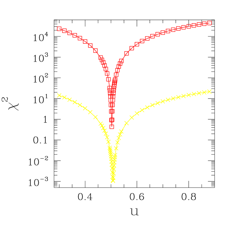
Figure 1: Semilogarithmic plot of $\chi^{2}$ against $u$ for least-squares fits of Eq.(9). Crosses: $\eta_{1}$; squares: $\eta_{2}$. Data for $\eta_{2}$ shifted upwards by a factor of 100 on vertical scale, to avoid superposition. For each fit, only data in the interval $3.05176E-10\leq x\leq 2.5E-06$ of Table 3 were used (see text).

Having ensured that square-root corrections to scaling are an essential element of the picture, we attempt to include higher-order terms, in the manner of Eq. (8). We plot $(\eta_{i}(x)-\eta_{i}(0))/\sqrt{x}$ against $\sqrt{x}$, thus one expects:

$$\frac{\eta_{i}(x)-\eta_{i}(0)}{\sqrt{x}}=C_{i}+D_{i}\,{\sqrt{x}}+{\cal O}(x)$$ (10)

and attempts straight-line fits. Results are in Figure 2.

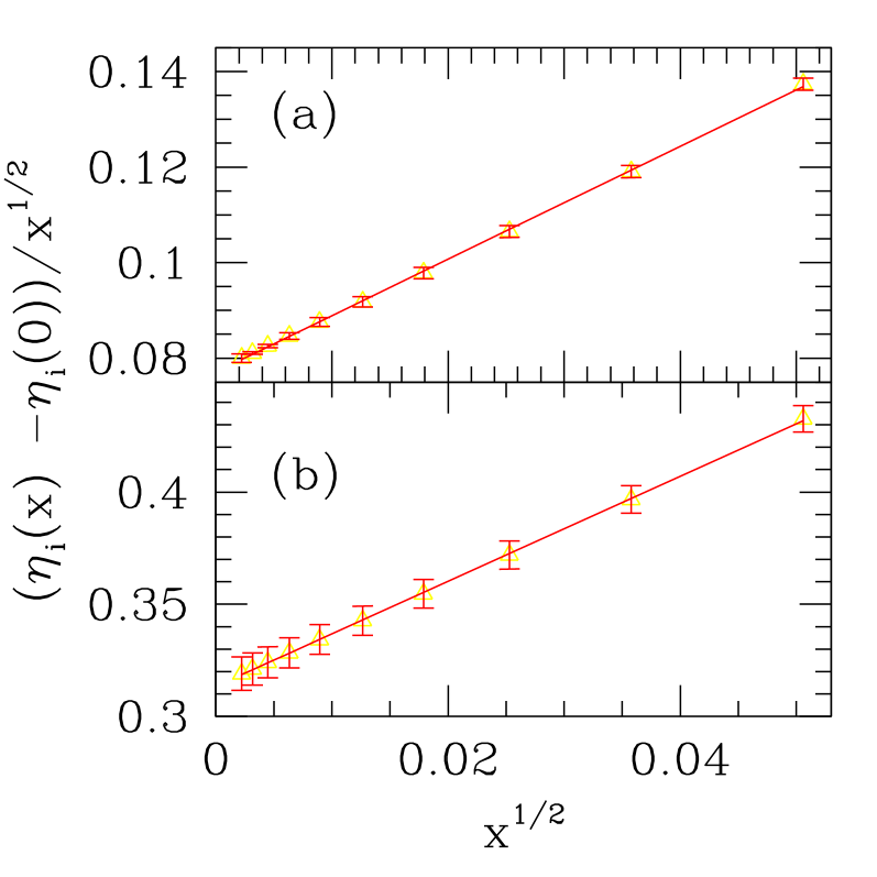
Figure 2: Plots of $(\eta_{i}(x)-\eta_{i}(0))/\sqrt{x}$ against $\sqrt{x}$, for $i=1$ (a) and $i=2$ (b). Straight lines are linear least-squares fits to the subset of data in plot, corresponding to $5.E-06<x<0.00256$ in Table 3 (see text).

The subset of data considered now is complementary to that used in the earlier single-power fits, as higher-order terms become more important for $x$ not very small. We noticed that inclusion of data from the last 3–4 lines of Table 3 caused a quick deterioration of the quality of linear fits (the resulting curvature can be seen by naked eye); this is probalbly the effect of third- and higher-order terms in $\sqrt{x}$. An alternative source of errors would be the multiplicative logarithmic terms, mentioned in connection with Eq. (8) above, and not considered in the present approach. Therefore, we decided to keep to the range of $x$ for which good linear plots were obtainable, while using as many data as possible (in order to reduce the spread in the estimates of $C_{i}$ and $D_{i}$ of Eq. (8)). The best compromise was found by taking data for $5.E-06<x<0.00256$, shown in Figure 2 together with the corresponding least-squares fits.

Table 4: Estimates of amplitudes $C_{i}$, $D_{i}$ (see Eqs. (8) –(10)), and $\chi^{2}$ per degree of freedom ($\chi^{2}/{\rm DOF})$ for respective fits.

	$C_{i}$	$D_{i}$	$\chi^{2}/{\rm DOF}$
Eq. (9), i=1, u=0.5	$0.079(4)$	$-$	$1.5\times 10^{-3}$
Eq. (10), i=1	$0.077(1)$	$1.18(3)$	$2\times 10^{-2}$
Eq. (9), i=2, u=0.5	$0.317(5)$	$-$	$3.0\times 10^{-3}$
Eq. (10), i=2	$0.313(3)$	$2.3(1)$	$2\times 10^{-3}$

Our estimates of the amplitudes $C_{i}$ and $D_{i}$ are shown in Table 4, where for single-power fits of Eq. (9) we quote only results for $u=0.5$. Although, as explained above, these do not correspond to the respective absolute minima of $\chi^{2}$, they exhibit a very good quality of fit, and it seems more appropriate to compare them (instead of those obtained at minimal $\chi^{2}$) to the estimates of $C_{i}$ from Eq. (10), where the power $1/2$ is fixed from the start.

IV Scaling of third gap

Finally, we have investigated the scaling of the third gap at $T=0$. According to theory dN82 ; saso98 , at the critical point there are only three relevant operators, corresponding (in decreasing order of relevance) to staggered magnetization, uniform magnetization and staggered polarization. Although, as recalled above, there is widespread agreement between theory and numerical work as regards the first two, the prediction of Ref. saso98, , namely that the corresponding decay-of-correlations exponent is $\eta_{{\bf P}_{\rm stagg}}=3$, appears not to have been numerically tested so far. ( In Ref. saso98, , Monte Carlo simulations were performed for the respective susceptibility, which according to the scaling law $\gamma/\nu=2-\eta$ is expected to approach a constant, with corrections $\propto L^{-\Delta}$, $\Delta=1$, if $\eta=3$; the approach to a constant was indeed verified, while the best fit was for $\Delta\simeq 0.75$ instead of unity).

We have calculated descending eigenvalues of the transfer matrix; it would seem plausible to associate the third scaled gap to the staggered polarization, especially since only three relevant operators are expected to come up, and the relationship of the other two to the first two gaps is well-established. In order to check self-consistency of our results, we used both a standard power-method algorithm, coupled with Gram-Schmidt orthogonalization, and a Lanczos scheme. While for small $L$ and shallow levels (corresponding to eigenvalues $\Lambda_{i}$, $i\leq 3$) both methods gave the same estimates, the Lanczos results displayed instabilities for deeper levels and $L\geq 8$. At present we are not able to explain such discrepancies. Therefore, we restrict ourselves to the analysis of the third gap.

Our results, again displayed in the form $\eta_{3}=L\,(\Lambda_{0}-\Lambda_{3})/\pi$, are shown in Table 5. In order to gain an unbiased perspective both of the limiting bulk value of $\eta_{3}$ and of the scaling corrections, we attempted a single-power extrapolation, $\eta_{3}(L)=\eta_{3}+a_{30}/L^{u}$ with a variable power $u$, and monitored the variations of the $\chi^{2}$ of the corresponding fits against $u$. The result was qualitatively very similar to that displayed for the fits of Eq. (9) in Fig. 1: a rather sharp minimum, located at $u=1.8$ in this case, which gave an extrapolated $\eta_{3}=2.00(1)$ (see Table 5; the error bar was calculated by considering the estimates on either side of $u_{\min}=1.8$, for which the $\chi^{2}$ becomes one order of magnitude larger than at the minimum). Fixing $u=1$, inspired by the prediction of Ref. saso98, for the susceptibility, gave $\eta_{3}\simeq 2.11$. Two-power fits à la Eq. (6), using either $L^{-2}$ and $L^{-4}$ or $L^{-1}$ and $L^{-2}$ also gave values between $1.99$ and $2.01$. There seems to be no straightforward way to extrapolate the data of Table 5 to include $\eta_{3}=3$ . At this point we do not know how to reconcile our results to the predictions of Ref. saso98, .

Table 5: Finite–$L$ and extrapolated estimates of $\eta_{3}$. The latter is the result of an equal-weight fit of data for $L=6$, $8\cdots 14$ respectively to a single-power ($L^{-u}$) correction; the corresponding $u=1.8$ was chosen to minimize the $\chi^{2}$ (see text).

L	$\eta_{3}$
6	1.74149553
8	1.84852826
10	1.90108612
12	1.93052844
14	1.94860339
Extr.	2.00(1)

V Conclusions

In summary, we have undertaken a finite-size approach to investigate the corrections to scaling in the three-state square-lattice Potts antiferromagnet. Owing to the characteristics of the quantities under study, we argued that the natural variable to consider is $x\equiv L\,e^{-2\beta}$. We showed that the less-relevant finite-size corrections could be accounted for in a phenomenological scheme, based on the zero-temperature picture; for the extrapolated scaled gaps we supplied convincing evidence that square-root corrections, in the variable $x$, are present, and provided estimates for the numerical values of the amplitudes of the first– and second–order correction terms, for both the first and second scaled gaps. It would be interesting if predictions based on theory could be derived, to be compared with the numerical values of amplitudes obtained in this work.

We have also investigated the behaviour of the third scaled gap of the transfer matrix spectrum, and found an extrapolated value for the decay-of-correlations exponent $\eta_{3}=2.00(1)$. This seems incompatible with earlier predictions, to the effect that the third relevant operator in the problem would give $\eta_{{\bf P}_{\rm stagg}}=3$, corresponding to the staggered polarization.

- (1) M. P. Nightingale and M. Schick, J. Phys. A 15, L39 (1982).
- (2) H. H. Roomany and H. W. Wyld, Phys. Rev. D21, 3341 (1980).
- (3) J.-S. Wang, R. H. Swendsen, and R. Kotecký, Phys. Rev. B42, 2465 (1990).
- (4) H. Saleur, Nucl. Phys. B 360, 219 (1991).
- (5) S. J. Ferreira and A. D. Sokal, Phys. Rev. B51, 6727 (1995).
- (6) S. L. A. de Queiroz, T. Paiva, J. S. de Sá Martins, and R. R. dos Santos, Phys. Rev. E59, 2772 (1999).
- (7) S. J. Ferreira and A. D. Sokal, J. Stat. Phys. 96, 461 (1999).
- (8) J. L. Cardy, J. L. Jacobsen, and A. D. Sokal, J. Stat. Phys. 105, 25 (2001).
- (9) J. L. Cardy, J. Phys. A 17, L385 (1984).
- (10) M. P. M. den Nijs, M. P. Nightingale and M. Schick, Phys. Rev. B26, 2490 (1982) .
- (11) J. Salas and A. D. Sokal, J. Stat. Phys. 92, 729 (1998).
- (12) M. N. Barber, in Phase Transitions and Critical Phenomena, edited by C. Domb and J.L. Lebowitz (Academic, New York, 1983), Vol. 8.
- (13) J. L. Cardy, Nucl. Phys. B 270, 186 (1986).
- (14) B. Nienhuis, J. Phys. A 15, 199 (1982).
- (15) S. L. A. de Queiroz, J. Phys. A 33, 721 (2000).