Luttinger liquid superlattices: realization of gapless insulating phases
Abstract
We investigate LL superlattices, a periodic structure composed of two kinds of one-dimensional systems of interacting electrons. We calculate several properties of the low-energy sector: the effective charge and spin velocities, the compressibility, various correlation functions, the Landauer conductance and the Drude weight. The low-energy properties are subsumed into effective parameters, much like homogeneous one-dimensional systems. A generic result is the weighted average nature of these parameters, in proportion to the spatial extent of the underlying subunits, pointing to the possibility of “engineered” structures. As a specific realization, we consider a one-dimensional Hubbard superlattice, which consists of a periodic arrangement of two long Hubbard chains with different coupling constants and different hopping amplitudes. This system exhibits a rich phase diagram with several phases, both metallic and insulating. We have found that gapless insulating phases are present over a wide range of parameters.
pacs:
71.10.Pm, 71.10.Fd, 71.30.+h, 73.22.-f, 73.63.-bI INTRODUCTION
The physics of one-dimensional electronic systems has been the subject of a vigorous onslaught recently, both theoretical and experimental. Experimentally, the ability to grow nanostructures such as quantum wiresTarucha et al. (1995); Yacoby et al. (1996); Fazio et al. (1998) and carbon nanotubesIijima (1991); Endo et al. (1996); T. W. Ebbesen (1997); S. J. Tans et al. (1997); Bockrath et al. (1997); Hamada et al. (1992) has enabled, for the first time, the investigation of systems of a truly one-dimensional nature. On the theoretical side, the peculiarities of the behavior of interacting electrons in one dimension have culminated in the proposal of a unique universality class dubbed the Luttinger liquidJ. M. Luttinger (1963); D. C. Mattis and E. H. Lieb (1965); A. Luther and I. Peschel (1974); J. Sólyom (1979); V. J. Emery (1979); F. D. M. Haldane (1981); J. Voit (1994) (LL), which stands in sharp contrast with the higher dimensional Fermi liquids established by Landau. The LL is characterized by the absence of stable quasi-particles, its low-energy sector being exhausted by collective charge and spin density excitations. Since the latter travel at different velocities, an added electron splits up into well separated charge and spin degrees of freedom. Furthermore, correlation functions decay in a power law fashion, with exponents set by only a few parameters. This generic behavior has been tested and confirmed in the case of edge transport in systems which exhibit the fractional quantum Hall effect.C. L. Kane and M. P. A. Fisher (1992); Moon et al. (1993); F. P. Milliken et al. (1996); A. M. Chang et al. (1996); Grayson et al. (1998) LL theory has also been successfully used to describe some low-energy properties of carbon nanotubes,Bockrath et al. (1998); Yao et al. (1999); R. Egger et al. (2001) though the situation in quantum wires remains controversial.O. M. Auslaender et al. (2000); D. W. Wang et al. (2001)
The effect of boundary conditions on the low-energy properties of LL’s was first considered several years ago.Fabrizio and A. O. Gogolin (1995) Moreover, the interplay between boundary, finite-size, and thermal effects has been shown to alter considerably the properties of the system.Eggert et al. (1996); A. E. Mattsson et al. (1997) In particular, the zero-temperature critical behavior of the bulk always crosses over to a boundary dominated regime. These studies are important to explain the experimental results of tunneling spectroscopy into one-dimensional systems. More recently, it has been proposed that one-dimensional systems with gapless degrees of freedom and open boundary conditions form a new universality class of quantum critical behavior called ‘bounded Luttinger liquids’.Voit et al. (2000)
A particular kind of boundary effect emerges in the case of inhomogeneities. In general, an inhomogeneous LL is modeled by allowing the velocities of collective excitations and and the correlation exponents and to vary in space. The absence of conductance renormalization in long high-mobility GaAs wires, for instance, has been analyzed and explained in terms of an inhomogeneous LL model, where the Fermi liquid leads are replaced by a non-interacting one-dimensional electron gas.D. L. Maslov and M. Stone (1995); I. Safi and H. J. Schulz (1995); V. V. Ponomarenko (1995); I. Safi and H. J. Schulz (1999); V. V. Ponomarenko and Nagaosa (1999) Furthermore, LL’s with different inhomogeneity profiles have also been used in the context of the fractional quantum Hall effect, to describe transitions between edge states at different fillings,A. M. Finkel’stein and Oreg (1995); D. B. Chklovskii and B. I. Halperin (1998) or between an edge state and a Fermi liquid.C. de C. Chamon and Fradkin (1997)
With an eye to practical applications as diodes or transistors, researchers have recently begun to fabricate heterojunctions of carbon nanotubesChico et al. (1996); P. G. Collins et al. (1997); Martel et al. (1998); S. J. Tans et al. (1998); Yao et al. (1999); Kılıç et al. (2000); A. N. Andriotis et al. (2001) which look especially promising. They happen to be another realization of an inhomogeneous one-dimensional system. Taking this idea one step further, we have been led to consider another kind of heterostructure: a superlattice. The effect of electronic correlations in superlattices was initiated through a one-dimensional Hubbard-like model called a Hubbard superlattice (HSL), Paiva and R. R. dos Santos (1996, 1998); Paiva and R. R. dos Santos (2000a) consisting of a periodic arrangement where the Hubbard on-site repulsion is turned on and off in a repeated fashion. Despite its simplicity, a number of remarkable features were found, in marked contrast with the otherwise homogeneous system: local moment weight can be transferred from repulsive to free sites, spin density wave (SDW) quasi-order is wiped out as a result of frustration, and strong SDW correlations (in a subset of sites) could set in above half-filling. Furthermore, the evolution of the local moment and of the charge gap, together with a strong-coupling analysis, showed that the electron density at which the system becomes a Mott insulator increases with the size of the free layer relative to the repulsive one. More recently, the possibility of a periodically modulated hopping at arbitrary filling and magnetization has been considered.D. C. Cabra et al. (2000)
In order to generalize the effects of a superlattice structure in an interacting one-dimensional system, we consider here a general Luttinger liquid superlattice (LLSL), making at first no reference to the underlying microscopic details. We show how its low-energy properties bear strong resemblance to a conventional Luttinger liquid. However, as in the case of bounded Luttinger liquids,Voit et al. (2000) new effective parameters have to be introduced, which are the superlattice analogues of the spin and charge velocities and stiffnesses. These encode all the information necessary for a description of the low-energy sector. Moreover, these effective parameters turn out to mix the properties of the underlying sub-units in proportion to their spatial extent. This spatial averaging characteristic suggests the possibility of fine-tuning the physical properties by a careful selection of the superlattice modulation, a feature which may prove useful in nano-device applications. We then consider specific realizations of the LLSL by analyzing in full detail a general HSL. We find a proliferation of phases, both metallic and insulating. Surprisingly, the insulating phases often have no charge gap, because additional charge can be accommodated in the compressible sub-units. A partial account of these results has appeared in Ref. J. Silva-Valencia et al., 2001.
The paper is organized as follows: In Sec. II, we introduce the bosonic formulation of the Tomonaga-Luttinger model and our model. We obtain the effective charge and spin velocities, the correlation functions with the effective exponents and the Drude weight for LL superlattices. The application of these results to various cases where the LL describes the low-energy sector of a Hubbard model is analyzed in Sec. III. We close with the conclusions in Sec. IV.
II THE MODEL
We briefly review the general aspects of a homogeneous LL in order to set up the notation. The low-energy, large-distance behavior of a one-dimensional fermionic system with spin-independent interactions is described by the HamiltonianJ. M. Luttinger (1963); D. C. Mattis and E. H. Lieb (1965); A. Luther and I. Peschel (1974); J. Sólyom (1979); V. J. Emery (1979); F. D. M. Haldane (1981); J. Voit (1994)
| (1) |
where is a short-distance cutoff, is the spin backward-scattering amplitude, and
| (2) |
with and for the charge and spin degrees of freedom, respectively.
The phase fields are
| (3) |
and
| (4) |
Here are the Fourier components of the charge- (spin-) density operator for the right- () and left- () branches of moving fermions. Introducing the total number operators (measured with respect to the ground state) for branch and spin , the total (charge and spin) number and current operators are
| (5) |
and
| (6) |
where the upper and lower signs correspond to and , respectively.
The operators and in Eqs. (1) and (2) obey Bose-like commutation relations: . Consequently, at least for , Eq. (1) describes independent long-wavelength oscillations of the charge and spin density, with linear dispersion relations , ( is the velocity of elementary excitations) and the system is conducting. The only nontrivial interaction effects in (1) come from the cosine term. However, for repulsive SU(2) invariant interactions (), this term is renormalized to zero in the long-wavelength limit, and at the fixed point one has . The three remaining parameters in (1) then completely determine the long-distance properties of the system; in particular, determines the long-distance decay of all the correlation functions of the system.
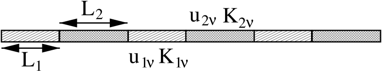
We now consider a LLSL, consisting of a repeated pattern of two different LL’s with parameters , and sizes () perfectly connected (Fig. 1). We use the adiabatic approximation, in which the scale of the inhomogeneity between the two liquids is much larger than the Fermi wavelength . Thus, the single-particle backscattering from the inhomogeneities can be neglected. Accordingly, the low-energy properties of this LLSL are described by generalizing the usual bosonized Hamiltonian of Eq. (1) as follows:
| (7) | |||||
where the sum extends over separated charge- () and spin- () degrees of freedom, each of which with interaction- and layer-dependent parameters and . For on the first (second) ‘layer’ one has () and ().
The boson phase fields are related to the charge and spin densities, and , through , while is such that is the momentum field conjugate to : . Note that in Eqs. (1) and (4).
The equations of motion for the fields and are
| (8) | |||||
| (9) |
which illustrate their duality under the replacement . Substituting (9) into (8) yields
| (10) |
and a similar equation for .
We now have to set up the matching equations at the interfaces between layers. The equations of motion lead to the continuity of and and their time derivatives. The right hand sides of Eqs. (8-9) yield, as additional conditions, the continuity of both and at the contacts. Note that the continuity of and guarantees that of the fermionic field.I. Safi and H. J. Schulz (1995); D. L. Maslov and M. Stone (1995); V. V. Ponomarenko (1995) Physically, these boundary conditions simply encode the conservation of both charge and spin currents (since we are neglecting Umklapp processes and backscattering of electrons with opposite spin). We stress that, under these conditions, these are the only universal requirements on the fields, irrespective of the actual interface potentials.
The superlattice structure is incorporated into the solution of the equations of motion in a way completely analogous to the discussion of reflection and transmission in the Kronig-Penney model. That is, we diagonalize the Hamiltonian (7) by expanding the phase fields in normal modes
| (11) | |||||
| (12) |
where , are boson creation operators (). The normal mode eigenfunctions and eigenvalues satisfy
| (13) |
[obtained by taking (11) into (10)], subject to the same boundary conditions at the contacts as before, with replacing . The eigenvalues are given by
| (14) | |||||
where and . For , the dispersion relation of the LLSL is linear, i.e., , with an effective velocity
| (15) |
where ; clearly, as , and as . Also, from Eq. (14) it follows that the spectrum of elementary excitations of a LLSL has bands and gaps, reflecting the superlattice structure. In this regard, it should be mentioned that, for a Luttinger liquid with a periodically modulated particle density, the presence of a plasmon gap was reported.A. Gramada and M. E. Raikh (1997) Here, we will focus only on the low energy properties of the LLSL.
On the other hand, the zero mode functions and , satisfy
| (16) | |||||
| (17) |
which follow from Eqs. (8) and (9). While for the homogeneous system one has
| (18) |
and
| (19) |
for the LLSL there will be, in general, an inhomogeneous periodic density profile. As we will see, there is a tendency for the charge to accumulate more in the less interactive layer. Thus, the zero mode functions will reflect this inhomogeneity.A. H. Castro Neto et al. (1997) Now, since each layer is a LL, and will vary in such a way that and across each layer , with layer-specific number and current operators. We then obtain
| (20) | |||||
| (21) |
where
| (22) |
with an analogous expression for obtained with the replacement of by . Here labels the unit cell. Analogously, from Eqs. (8) and (9) we have
| (23) | |||||
| (24) |
In a LL, the ground state value of measures the charge compressibility, whereas is related to the spin susceptibility. Considering the LLSL zero modes [Eqs. (20) and (21)] and the Hamiltonian (7) we find that the superlattice compressibility is given by
| (25) |
where is the compressibility of each layer. Clearly is nothing but an average of the individual compressibilities weighted by the layer lengths.
Interactions in a one-dimensional system can enhance charge density or superconducting fluctuations depending on whether they are repulsive or attractive. Let us then consider the correlation functions for the LLSL at . The asymptotic (i.e., for well separated and ) behavior of the density-density correlation function is
| (26) | |||||
where
| (27) | |||||
| (28) |
and . The second and third terms on the right-hand side of Eq. (26) respectively correspond to the and correlations in the homogeneous case. And, similarly to the homogeneous system, the former dominate over the latter for (see, however, Ref. Paiva and R. R. dos Santos, 2000b).
The correlation functions for spin-spin, singlet (SS) and triplet (TS) superconducting pairing are given by
| (29) | |||||
| (30) | |||||
| (31) | |||||
| (32) |
where [Eq. (27)], reflecting the duality properties (in the homogeneous limit we have ). One should note that the correlation functions depend not only on the difference , but also on the actual positions and , through the zero mode functions. It is interesting to note that, even though we now have new effective coupling constants (,), the scaling laws between the exponents of the correlation functions are not broken by the superlattice structure. In other words, the replacement and in the exponents of the correlation functions of the homogeneous system yields the exponents given above for the superlattice.
Finally, we discuss the conducting properties. Let us first consider a LLSL in the presence of a weak external space- and time-dependent electrostatic potential , such that the electric field . The interaction of the fermions with is described by a source term
| (33) |
Now the equation of motion for isI. Safi and H. J. Schulz (1995, 1999); D. L. Maslov and M. Stone (1995); V. V. Ponomarenko (1995)
| (34) |
Defining the bosonic Green’s function
| (35) |
the nonlocal conductivity is given by
| (36) |
where is the conductance quantum. First, we consider the usual order of limits, taking before which yields the Drude weight, appropriate for a situation of a uniform static electric field.E. W. Fenton (1992) In this case
| (37) |
which has the same form as for the homogeneous case,H. J. Schulz (1990) but with the effective velocity and effective exponent replacing the corresponding uniform quantities and . Taking the limits in the reverse order yields the Landauer conductance, which corresponds to a situation where an electric field is applied to a finite region of the sample.E. W. Fenton (1992) In the LLSL we have
| (38) |
which is similar to the homogeneous case,Apel and T. M. Rice (1982) except that the effective exponent appears. Naturally, the conductance renormalization of Eq. (38) is usually hidden in the presence of Fermi liquid leads.D. L. Maslov and M. Stone (1995); V. V. Ponomarenko (1995); I. Safi and H. J. Schulz (1995) However, it should be accessible in AC measurements, if , the inverse traversal time of the sample.K. A. Matveev and L. I. Glazman (1993)
III Hubbard Superlattices
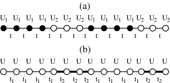
For the sake of illustrating the LLSL with a specific realization, we now discuss a one-dimensional Hubbard superlattice (HSL).Paiva and R. R. dos Santos (1996, 1998); Paiva and R. R. dos Santos (2000a); D. C. Cabra et al. (2000) We first consider a periodic arrangement of sites in which the on-site coupling is , followed by others with on-site coupling ; the hopping parameter, , is uniform, as shown in Fig. 2(a). We subsequently consider the on-site interaction as being uniform but the hopping integrals as periodic: between sites, followed by between sites; see Fig. 2(b).
Both cases above are contemplated if one writes the Hamiltonian as
| (39) |
where, in standard notation, runs over the sites of a one-dimensional lattice, creates (annihilates) a fermion at site in the spin state or and . It is important to notice that the SL structure breaks particle-hole symmetry.Paiva and R. R. dos Santos (2000a) The homogeneous Hubbard model, in a grand-canonical ensemble description, is invariant under a particle-hole transformation only when . In the superlattice case, a uniform chemical potential cannot ensure this symmetry throughout the whole system. Instead, under a particle-hole transformation the system is mapped onto a different one with a spatially modulated chemical potential.
A weak coupling perturbation theory, similar to that for the homogeneous model can be used to show that Eq. (7) indeed describes the low energy and small momentum sector of the discrete model of Eq. (39) in the limit of long layers; see the Appendix. Then, in Eq. (7) one has and for on the layer , where and are the usual uniform weak coupling LL parameters for each layer. It is by now well established that a LL description is appropriate for the low-energy sector of the Hubbard model, even in the strong coupling limit .H. J. Schulz (1990) Now, each long Hubbard sub-chain is still a finite-sized LL, though connected to particle reservoirs at each end.A. H. Castro Neto et al. (1997) We therefore make the quite reasonable assumption that the above LLSL description remains valid even in the strong coupling limit. With respect to magnetic properties, the superlattice structure (with repulsive interactions) does not break SU(2) symmetry, so that the inhomogeneous is still expected to renormalize to .
Because each sub-chain is an open LL, there will be a certain amount of charge redistribution between them, leading to a non-uniform charge profile. Let us first consider the special case of two layers only [with parameters and ] initially disconnected and with the same initial density . In general, these two sub-systems will not have the same chemical potential. We then bring them in contact with each other, so that particle exchange is allowed. Electrons will flow from one system to the other until their chemical potentials exactly match:
| (40) |
where and are the chemical potential and the equilibrium densities of each layer, respectively. This is just the condition for thermodynamic equilibrium. Naturally, conservation of total charge dictates that
| (41) |
In order to determine and , we must solve simultaneously Eqs. (40) and (41). The extension to the case of more than two layers leads to no modifications of the above equations and the charge profile will be periodic with the densities determined as above.
The dependence of on the density and on the interaction can be obtained from the exact solution of the homogeneous Hubbard model.E. H. Lieb and F. Y. Wu (1968) As a function of , the chemical potential increases monotonically and is discontinuous at half-filling, where it jumps from to . Thus, the homogeneous model is a Mott insulator at half-filling. is the lower chemical potential at half-filling, given byE. H. Lieb and F. Y. Wu (1968)
| (42) |
where is a Bessel function. To increase the particle number above half-filling, we need to pay an energy given by
| (43) |
which is the quasiparticle gap. For later use, we also quote the chemical potential of the non-interacting case,
| (44) |
III.1 The case
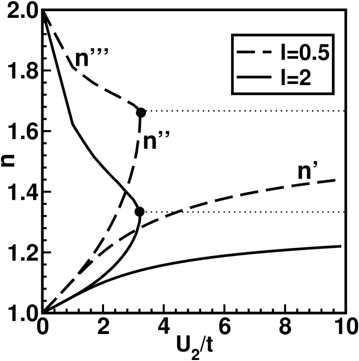
We first consider the case in which one of the layers is ‘free’ () and take for simplicity. Figure 3 shows the phase diagram for and 2; the case has been discussed in Ref. J. Silva-Valencia et al., 2001. For the sake of comparison, one should also keep in mind the phase diagram for the homogeneous LL, in which there is a single gapped (Mott) insulating phase for any non-zero repulsion at half-filling; upon either electron- or hole-doping the system becomes metallic. In what follows, we start with a qualitative discussion of the phase diagram, after which we provide the details of how the boundaries and special points are determined.
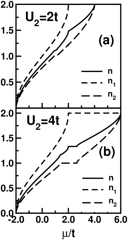
In the case of a superlattice, while for the system is always metallic, interesting metal-insulator transitions have been found for , as displayed in Fig. 3. Indeed, for a density just above half-filling, the system is still metallic, with more particles occupying the free layer than the repulsive one in order to decrease the overall electronic repulsion: One has and , as shown in Fig. 4. As the density is increased for given and , electrons will be accommodated in both layers without affecting the metallic character; see Figs. 3 and 4. This will persist until the repulsive layer is half filled (), when it becomes a Mott insulator. Recall that an insulating phase in one of the subsystems is signalled in Fig. 4 by a horizontal plateau in the corresponding ( 2) plots. The system as a whole is therefore an insulator, since it can be thought of as a series arrangement of resistors. However, the unusual fact is the gapless nature of this insulating phase: charge can be accommodated in the free layer at no energy cost, since the system is compressible () in this range of ; see Fig. 4.
As the density is further increased, the system responds in two different ways, depending on whether is larger or smaller than (for all ); see Figs. 3 and 4. If [Fig. 4(a)], the insulating state can only be sustained up to a limited amount of additional charge; that is, as long as it is energetically favorable to accommodate this extra charge in the free layer, while keeping . Further increase in soon leads to an increase in the occupation of the repulsive layer (with ) and the system reenters an overall metallic phase. This metallic character will be lost again for larger , when the free layer becomes completely full (), with the superlattice displaying insulating behavior. Again, this insulating phase is gapless.
If [Fig. 4(b)], on the other hand, all added electrons will be accommodated in the free layer (), so that the superlattice remains in the state of a gapless insulator. Further increase in the electron density leads to the free layer becoming a band insulator (), while keeping the repulsive one pinned at half-filling; the density, , at which this occurs depends on the aspect ratio, , and is given by [c.f., Eq. (41) and Refs. Paiva and R. R. dos Santos, 1998; Paiva and R. R. dos Santos, 2000a] . Only at this special density does the superlattice become a Mott insulator, since it is incompressible (); see Fig. 4(b). For , the free layer remains completely full, so that all added electrons go to the repulsive layer; the superlattice behaves again as a gapless insulator.
At this point it is worth commenting that the phase diagram of Fig. 3 differs in two aspects from the one found for thin layers, obtained by means of Lanczos diagonalizations: In Ref. Paiva and R. R. dos Santos, 1998 no gapless insulating phases were probed, and the insulating phase for was found to extend down to any . The former difference is due to the fact that only gapped insulating phases were probed, while the latter can be traced back to finite-size effects.
Let us now fill in the details on how the lines and special points of Fig. 3 are determined. The dotted horizontal line at is obtained by setting both and . However, this condition can only be obtained if where is determined implicitly by (see Fig. 4)
| (45) |
Since neither Eq. (45) nor Eq. (42) depends on , this condition yields the same for any finite aspect ratio.
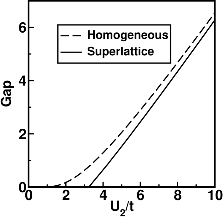
Besides, for , the system is always gapless. For and the system shows a Mott-Hubbard gap given by the energy difference between the highest occupied state, which is the upper edge of the non-interacting band at , and the lowest unoccupied level, which is the higher chemical potential of the half-filled Hubbard chain at
| (46) |
For the one-dimensional Hubbard model, one has in weak coupling and in strong coupling. For the HSL, we found that is linear with for large and is always lower than the gap of the corresponding homogeneous system; see Fig. 5.
The two metallic phases are characterized by (lower one) and (upper one). The metal-insulator transition (MIT) lines can therefore be obtained by means of Eqs. (40), (41), the Lieb-Wu chemical potential and (44). Therefore, in Fig. 3, (i) is the line in which the lower Hubbard band of the interacting sub-chain becomes fully occupied, (ii) is the one in which the upper Hubbard band starts to fill, and (iii) is the line in which the non-interacting sub-chain fills up. Thus,
| (47) | |||||
| (48) | |||||
| (49) |
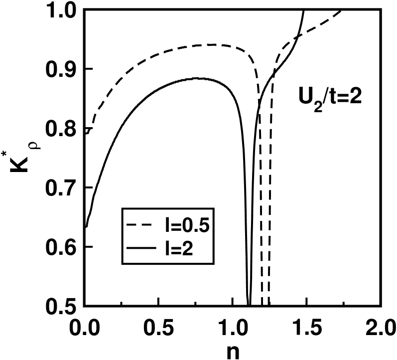
The LL description of Sec. II is only valid in the metallic regions of the phase diagram, where no gap is present in either the spin or the charge sectors. In these regions, we have
where is the Fermi velocity. When the insulating phase is approached from the lower metallic region (see Fig. 3), as a result of in the interacting layer. In Fig. 6, we show the effective exponent as a function of the filling . For any , both metallic phases have and the charge and spin correlation functions decay faster than in the homogeneous system. This is a direct consequence of the ‘weighted average’ character of the effective exponent . By the same token, for a given on the lower metallic phase, decreases as increases. In the upper metallic phase, always tends to the non-interacting value of 1 as the upper insulating region is approached; for the superlattice with larger reaches 1 at a lower overall density.
III.2 The general case:
We now consider a more general HSL, with different non-vanishing coupling constants on each layer (), while keeping the same hopping amplitude throughout the lattice (Fig. 2(a)). Using once again the exact expression for the chemical potential as a function of both and ,E. H. Lieb and F. Y. Wu (1968) we have determined the charge profile of the superlattice system. The charge tends to accumulate in the layer with the smaller coupling, which we choose to call layer 1. This is rather intuitive, since electrons decrease their mutual repulsion energy by flowing into the less interacting layer.
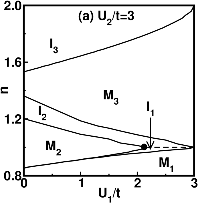
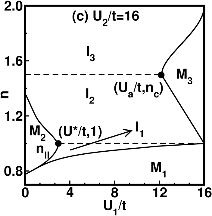
The phase diagram for this HSL is very rich. We observe six different phases, three metallic (M1, M2 and M3) and three insulating (I1, I2 and I3), each characterized by its charge profile, as shown for three illustrative cases in Fig. 7. The topology of the phase diagram is the same for any and the limiting cases (Section III.1) and (homogeneous chain) are recovered. On each phase diagram of Fig. 7, there are five MIT lines, labeled by through , which are determined similarly to the case discussed before (see Table 1). We get:
line I:
| (50) |
line II:
| (51) |
line III:
| (52) |
line IV:
| (53) |
line V:
| (54) |
For , the lines and determine the phase diagram of Section III.1 [Eqs. (47)–(49)].J. Silva-Valencia et al. (2001)
One of the consequences of a non-zero is to push the lower metallic phase of Fig. 3 to smaller densities, as shown in Fig. 7 (M1). In addition to this phase, which spans all values of , there are two other metallic regions (M2 and M3). And in-between metallic phases, one finds insulating phases, one of which (I1) is now stable for , unlike the case for . These insulating phases have either or (see Table 1). Once again, there is a ‘division of labor’ between the two types of sub-chains: while one is gapped (Mott) or completely filled (band), being responsible for the insulating behavior of the system, the other remains gapless and so does the system as a whole.
| Sub-chain densities | Transition line | |
|---|---|---|
| M1 | , | - |
| - | LHB 1 fills up () | |
| I1 | , | - |
| - | UHB 1 starts to fill () | |
| M2 | , | - |
| - | LHB 2 fills up () | |
| I2 | , | - |
| - | UHB 2 starts to fill () | |
| M3 | , | - |
| - | UHB 1 fills up () |
Figure 7(a) shows the phase diagram for ( is the same as for the case ). The HSL has a gap at the density for ; this line separates the I1 (i.e., , ) and the I2 (, ) gapless insulating phases. For one goes through a sequence of MIT’s, in which all insulating phases are gapless.
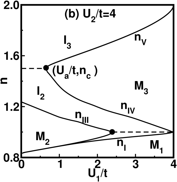
In Fig. 7(b), we show the phase diagram for . As the overall density is increased from 1 in the interval , where and , the system goes through a sequence of MIT’s without ever being gapped. However, for , the intermediate I2 (, ) and the I3 (, ) gapless insulating phases are separated by the dashed line at the density , where the system is fully gapped. Similarly, another gap appears at the density for , which again separates gapless insulating phases I1 (, ) and I2 (, ).
For [Fig. 7(c)] and (now and ) the system is metallic only below line , which approaches for large ; also, gapped behavior is again observed at densities and , with all other insulating phases being gapless. For each of the regions and , a ‘tipped’ metallic phase is observed.
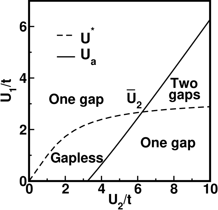
The above discussion indicates that there are special values of , and , which respectively represent the ‘tip’ positions of the low- and high-density metallic phases. Their dependence on can be extracted from the solutions of
| (55) |
and of
| (56) |
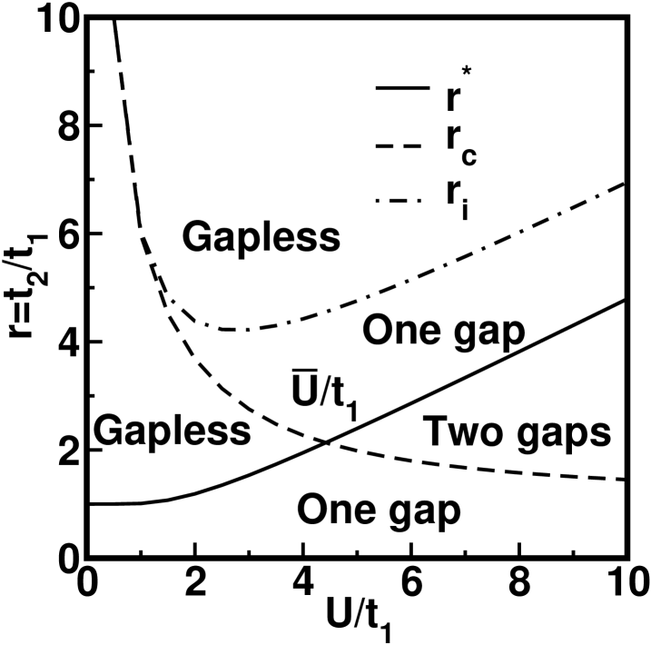
and are shown in Fig. 8. It should be noted that these values are independent of the aspect ratio . As Fig. 8 reveals, one should not be misled by the different horizontal scales in Fig. 7: the low-density tip does not recede as increases, since actually increases monotonically with , saturating at as . On the other hand, Fig. 8 shows that is only defined above a certain threshold, , reflecting the fact that when the coupling in layer 2 is small, the situation is never realized; above , increases linearly with .
According to our previous analyses, these two curves (which intersect at ) define regions in the plane characterized by the number of gaps in the sub-units for appropriate fillings, as specified in Fig. 8.
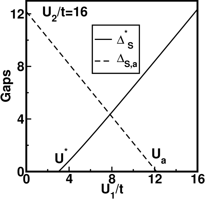
Similarly to the case , the gaps at the densities and are given, respectively, by
| (57) | |||||
| (58) |
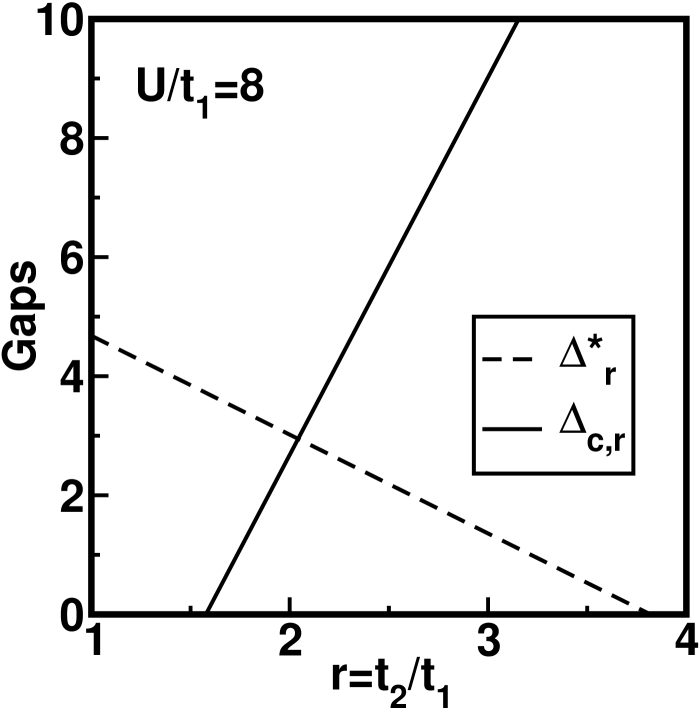
and, again, they do not depend on . The gaps and , for , are shown in Fig. 9 as functions of . The gap at [] increases [decreases] linearly with and vanishes for [].
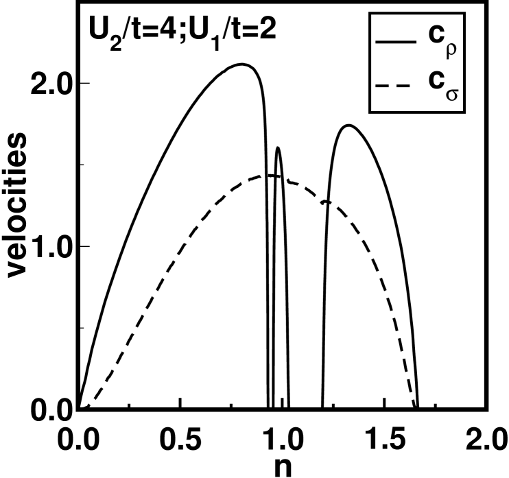
For the Hubbard model with repulsive interactions we have and .H. J. Schulz (1990) For and , the effective charge and spin velocities for the one-dimensional Hubbard superlattice are shown in Fig. 10 as functions of . The effective charge velocity (full line in Fig. 10) vanishes upon approaching the insulating regions as a result of the vanishing charge velocities of the individual sub-chains . Thus, shows a re-entrant behavior as a function of (cf. Fig. 7). As in the homogeneous case, the effective spin velocity is always smaller than the Fermi velocity and only vanishes in the upper insulating phase (dashed line in Fig. 10). The different behaviors of and can be traced back to the the fact that is sensitive to the superlattice structure, while , since as a result of the SU(2) symmetry being preserved.
The preservation of SU(2) symmetry also leads to . Thus, from Eqs. (26) and (29), the density-density and spin-spin correlation functions for the HSL are dominated by . These terms correspond to -CDW and -SDW in the homogeneous system. Here, and the density-density and spin-spin correlation functions for the HSL decay faster (slower) than for a homogeneous system with (). Similarly, pairing correlation functions are . In spite of the presence of effective exponents and , the condition for superconducting quasi-long range order is again , analogous to the homogeneous case; this condition, nonetheless, remains unsatisfied.
In Fig. 11, the correlation exponent of the HSL is shown as a function of band filling, for different superlattices: HSL-1 with t and ; HSL-2 with and ; HSL-3 with and . For any , all metallic phases are characterized by . We note that HSL-1 has three metallic phases, HSL-2 has two metallic phases and HSL-3 has only one metallic phase. On the low density side, approaches 1/2 in contrast to the case (Sec. III.1), in which remains between 1/2 and 1. From Eq. (27) one sees that interpolates monotonically between and as is varied from 0 to , highlighting the possibility of a continuous ‘modulation’ of a physical parameter through the tuning of the superlattice structure.
III.3 Two different hoppings: and
We now consider two Hubbard chains arranged periodically with the same coupling , but different hoppings (Fig. 2(b)).D. C. Cabra et al. (2000)
Initially, the charge tends to accumulate in the layer with larger hopping (layer 2), because its chemical potential is the smallest. Eventually, their chemical potentials become equal at the special density , determined by . Then, for , the charge flow is reversed and proceeds from layer 2 to layer 1. is independent of and , and decreases with (see Fig. 12).
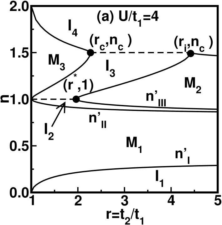
It is interesting to plot a phase diagram in terms of the density and the ratio between the two hopping amplitudes, . We then identify seven different phases, three metallic (M1, M2 and M3) and four insulating (I1, I2, I3 and I4), as shown in Fig. 12 for and with and listed in Table 2. The value of lies within the M1 phase. We mention that several different insulating and metallic phases were also found in a p-merized Hubbard chain in a magnetic field.D. C. Cabra et al. (2000)
| Sub-chain densities | Transition line | |
|---|---|---|
| I1 | , | - |
| - | LHB 1 starts to fill () | |
| M1 | , | - |
| - | LHB 1 fills up () | |
| I2 | , | - |
| - | UHB 1 starts to fill () | |
| M2 | , | - |
| - | LHB 2 fills up () | |
| I3 | , | - |
| - | UHB 2 starts to fill () | |
| M3 | , | - |
| - | UHB 1 fills up () | |
| I4 | , | - |
Following the same reasonings as before, the lines in the phase diagram in Fig. 12 are given by:
line I:
| (59) |
line II:
| (60) |
line III:
| (61) |
line IV:
| (62) |
line V:
| (63) |
line VI:
| (64) |
Again, the topology of the phase diagrams in Fig. 12 is the same for any .
At small densities (I1 phase), charge accumulates in layer 2 while layer 1 is empty (); the system is therefore a gapless insulator.
As the density increases, layer 1 only starts being filled at , determined by Eq. (59), which locates a transition to a metallic state (M1); see Fig. 12. Further increase in the overall density leads to an increase in both and . When layer 1 becomes half-filled, which occurs at as determined from Eq. (60), the system reenters a gapless insulating state (I2). If , where
| (65) |
upon increasing the density the system goes through a gapped phase at . The dependences of with , and of the gap at ,
| (66) |
with , are shown in Figs. 13 and 14, respectively; note that and . By contrast, if , the system enters a metallic phase (M2) bounded by , and , given by Eqs. (61) and (62).
When increasing the density above half filling, the sequence of phases depends crucially on whether is smaller or larger than
| (67) |
which, according to Fig. 13, occurs when or when respectively.
Let us first consider , which is the situation of Fig. 12(a). If , one goes through two transitions as increases: I M3 at [see Eq. (63)], and M I4 at [Eq. (64)]. If , the sequence is M2-I3-M3-I4, until the lattice is completely filled. Another regime is determined by
| (68) |
whose dependence on is also shown in Fig. 13. If , the system goes from a metallic (M2) to a gapless insulating phase (I3), and then, at , another Mott-Hubbard gap opens, which is given by
| (69) |
For a fixed ratio , behaves as shown in Fig. 14. Above , the gapless insulating state I4 is again stabilized. It should also be noted that both gaps ( and ) display universal behavior in the sense that they do not depend on . Note also that Eqs. (65), (67), and (68) do not depend on , so that is also universal.
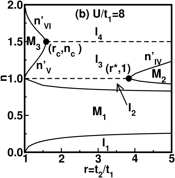
We now consider , an example of which is shown in Fig. 12(b). For , one finds the same sequence I3-M3-I4, with all insulating phases being gapless. If , a gapped insulating phase is crossed at . Similarly, for one goes from a metallic to a gapless insulating phase (M I3), and again crossing the Mott-Hubbard phase at .
The effective charge and spin velocities are given by
| (70) |
which vanish for and are smaller than the velocities of the homogeneous system (). Furthermore, displays re-entrant behavior as a function of .
Finally, the effective interaction parameter is
| (71) |
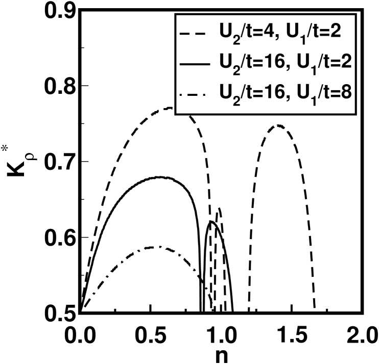
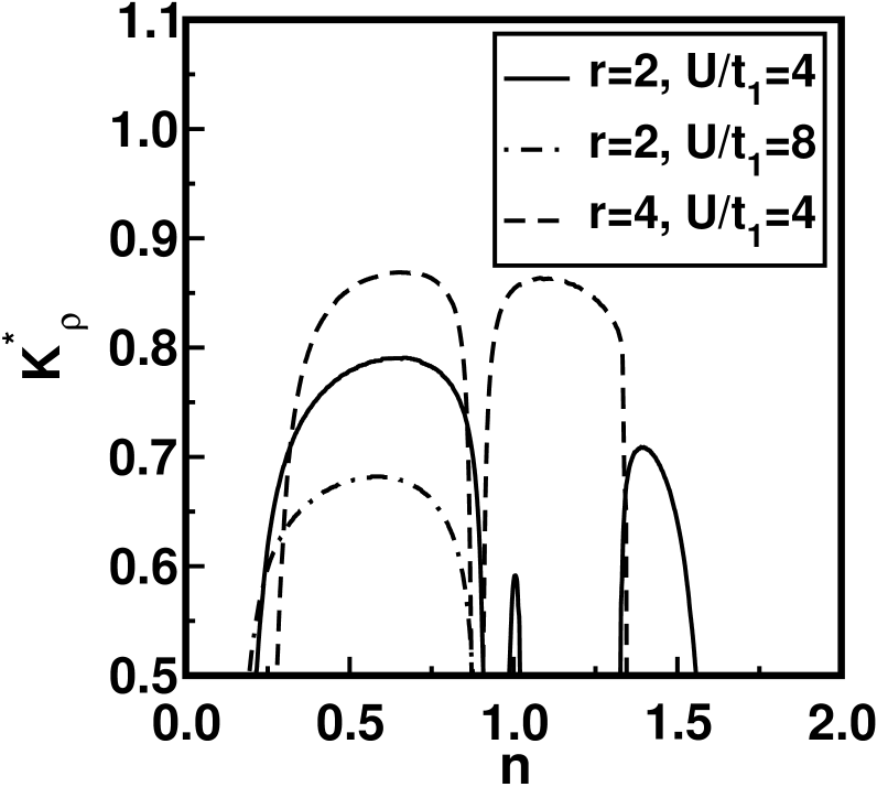
In Fig. 15, is shown as a function of band filling, for different couplings in superlattices with : HSL-A with and ; HSL-B with and ; HSL-C with and . Note that for any in the metallic phases. The various cases depicted in Fig. 15 show three (A), one (B) and two (C) metallic phases. In the homogeneous Hubbard chain, the density-density and spin-spin correlation functions decay faster when the hopping increases, since increases with the ratio . The effective correlation exponent of HSL-C is larger than in HSL-A (see Fig. 15), because of the larger hopping amplitude of sub-chain 2 in HSL-C and the ‘averaging’ nature of .
We should stress that in the homogeneous system, the Luttinger Liquid description breaks down at half-filling, when a gap opens in the charge (though not in the spin) sector. In the superlattice, this breakdown occurs in the insulating phases, as a result either of Umklapp processes (Mott gap, lower phase of Fig. 3, phases I1 and I2 of Fig. 7 and phases I2 and I3 of Fig. 12), or of a band in one of the sub-lattices becoming completely full or empty (upper phase of Fig. 3, phase I3 of Fig. 7 and phases I1 and I4 of Fig. 12),
IV CONCLUSIONS
We have discussed in full generality the properties of Luttinger liquid superlattices. We have seen how most features of a conventional Luttinger liquid description survive in the superlattice structure. In particular, a few effective parameters, the spin and charge velocities ( and ) and the stiffnesses ( and ) are all that is required for a complete description of the low-energy sector. These turn out to be combinations of the LL parameters of the superlattice sub-units combined in proportion to their spatial extent. As we have stressed in the Introduction, this opens the way for possible ‘engineering’ of Luttinger liquids.
This framework was applied to the study of the general phase diagram of Hubbard superlattices. It was then illustrated how one can tune between different phases by an appropriate choice of superlattice modulation. It was found that the superlattice displays a variety of metallic and insulating phases, the most prominent feature being the appearance of gapless insulating phases, as a result of the one-dimensional character of the system; gapped insulating phases were also found at some special densities.
Single-wall metallic carbon nanotubes (SWMN’s) seem to provide a promising route towards realizing these LLSL’s. Indeed, notwithstanding the fact that SWMN’s are, in general, described by a less simplistic model (possibly even with more branchesR. Egger et al. (2001); Egger and A. O. Gogolin (1997)), the LL coupling constant depends on its (true) aspect ratio throughR. Egger et al. (2001)
| (72) |
where is the dielectric constant, and and are, respectively, the nanotube length and radius; typically one has -0.3. More recently, the growth of intramolecular junctions of SWMN’s with different radii has been achieved with the introduction of a pentagon and a heptagon into the hexagonal carbon lattice,Chico et al. (1996); P. G. Collins et al. (1997); Martel et al. (1998); S. J. Tans et al. (1998); Yao et al. (1999); Kılıç et al. (2000); A. N. Andriotis et al. (2001) so that the fabrication of a superlattice made up of SWMN’s with different coupling constants has become a concrete possibility.
We therefore expect the phase diagram of this ‘nanotube array’ to share several features with the general Hubbard superlattice. This is because the only ingredients that enter into the phase determination are the thermodynamic equilibrium condition and charge conservation. In the case of a Luttinger liquid these can be easily written down if one knows how the LL parameters depend on the density
Thus, the sequence of insulating and metallic phases that we have found in Hubbard superlattices should be present in other systems as well, as they will reflect the phase diagram of the sub-units. We hope this rich variety of behaviors will stimulate further experimental work along the lines of carefully controlled nanotube arrays.
Acknowledgements.
The authors are grateful to A.O. Caldeira, A.L. Malvezzi, and T. Paiva for discussions. Financial support from the Brazilian Agencies CNPq, FAPESP (E.M.), and FAPERJ (R.R.d.S.) is also gratefully acknowledged.*
Appendix A Weak coupling bosonization of a Hubbard Superlattice
Here we consider a Hubbard superlattice in weak coupling and show that it is possible to describe the low-energy properties in terms of a Luttinger liquid superlattice. The Hamiltonian of a Hubbard superlattice is
| (73) | |||||
We focus on the low energy modes near the Fermi surface, so that each fermion is written asJ. Voit (1994)
| (74) |
where is the lattice parameter, and the subscripts and respectively denote right and left movers. The kinetic energy part is then linearized as in the homogeneous case
The fermionic fields are given in terms of the bosonic ones, , asJ. Voit (1994)
Here is a cutoff parameter and is the Klein factor.F. D. M. Haldane (1981); J. Voit (1994) Thus we get
| (76) |
where and
| (77) |
We now work out the low energy part of the on-site Hubbard interaction. Again, we use Eq.(74) to get
| (78) | |||||
where denotes normal ordering,J. Voit (1994) , and the Umklapp terms have been neglected. Then
where h.c. stands for hermitian conjugate. In terms of charge () and spin () fields we have
| (80) | |||||
the last term corresponding to the spin backscattering interaction, which is irrelevant in the RG sense. Finally, the low energy Hamiltonian for the Hubbard superlattice is
This has the same form as Eq. (7), which describes the Luttinger liquid superlattice.
References
- Tarucha et al. (1995) S. Tarucha, T. Honda, and T. Saku, Solid State Commun. 94, 413 (1995).
- Yacoby et al. (1996) A. Yacoby, H. L. Stormer, N. S. Wingreen, L. N. Pfeiffer, K. W. Baldwin, and K. W. West, Phys. Rev. Lett. 77, 4612 (1996).
- Fazio et al. (1998) R. Fazio, F. W. J. Hekking, and D. E. Khmelnitskii, Phys. Rev. Lett. 80, 5611 (1998).
- Iijima (1991) S. Iijima, Nature 354, 56 (1991).
- Endo et al. (1996) M. Endo, S. Iijima, and M. S. Dresselhaus, Carbon Nanotubes (Pergamon, Oxford, 1996).
- T. W. Ebbesen (1997) T. W. Ebbesen, Carbon Nanotubes (CRC Press, Boca Raton, Florida, 1997).
- S. J. Tans et al. (1997) S. J. Tans, M. H. Devoret, H. J. Dai, A. Thess, R. E. Smalley, L. J. Geerligs, and C. Dekker, Nature 386, 474 (1997).
- Bockrath et al. (1997) M. Bockrath, D. H. Cobden, P. L. McEuen, N. G. Chopra, A. Zettl, A. Thess, and R. E. Smalley, Science 275, 1922 (1997).
- Hamada et al. (1992) N. Hamada, S. Sawada, and A. Oshiyama, Phys. Rev. Lett. 68, 1579 (1992).
- J. M. Luttinger (1963) J. M. Luttinger, J. Math. Phys. 4, 1154 (1963).
- D. C. Mattis and E. H. Lieb (1965) D. C. Mattis and E. H. Lieb, J. Math. Phys. 6, 304 (1965).
- A. Luther and I. Peschel (1974) A. Luther and I. Peschel, Phys. Rev. B 9, 2911 (1974).
- J. Sólyom (1979) J. Sólyom, Adv. Phys. 28, 201 (1979).
- V. J. Emery (1979) V. J. Emery, in Highly conducting one-dimensional solids, edited by J. T. Devreese, R. P. Evrard, and V. E. van Doren (Plenum, New York, 1979), chap. 6, pp. 247–303.
- F. D. M. Haldane (1981) F. D. M. Haldane, J. Phys. C 14, 2585 (1981).
- J. Voit (1994) J. Voit, Rep. Prog. Phys. 57, 977 (1994).
- C. L. Kane and M. P. A. Fisher (1992) C. L. Kane and M. P. A. Fisher, Phys. Rev. B 46, 7268 (1992).
- Moon et al. (1993) K. Moon, H. Yi, C. L. Kane, S. M. Girvin, and M. P. A. Fisher, Phys. Rev. Lett. 71, 4381 (1993).
- F. P. Milliken et al. (1996) F. P. Milliken, C. P. Umbach, and R. A. Webb, Solid State Commun. 97, 309 (1996).
- A. M. Chang et al. (1996) A. M. Chang, L. N. Pfeiffer, and K. W. West, Phys. Rev. Lett. 77, 2538 (1996).
- Grayson et al. (1998) M. Grayson, D. C. Tsui, L. N. Pfeiffer, K. W. West, and A. M. Chang, Phys. Rev. Lett. 80, 1062 (1998).
- Bockrath et al. (1998) M. Bockrath, D. H. Cobden, J. Lu, A. G. Rinzler, R. E. Smalley, L. Balents, and P. L. McEuen, Nature 397, 598 (1998).
- Yao et al. (1999) Z. Yao, H. W. C. Postma, L. Balents, and C. Dekker, Nature 402, 273 (1999).
- R. Egger et al. (2001) R. Egger, A. Bachtold, M. S. Fuhrer, M. Bockrath, D. H. Cobden, and P. L. McEuen, in Interacting Electrons in Nanostructures, edited by R. Haug and H. Schoeller (Springer, 2001), cond-mat/0008008.
- O. M. Auslaender et al. (2000) O. M. Auslaender, A. Yacoby, R. de Picciotto, K. W. Baldwin, L. N. Pfeiffer, and K. W. West, Phys. Rev. Lett. 84, 1764 (2000).
- D. W. Wang et al. (2001) D. W. Wang, A. J. Millis, and S. das Sarma, Phys. Rev. Lett. 85, 4570 (2000).
- Fabrizio and A. O. Gogolin (1995) M. Fabrizio and A. O. Gogolin, Phys. Rev. B 51, 17827 (1995).
- Eggert et al. (1996) S. Eggert, H. Johannesson, and A. Mattsson, Phys. Rev. Lett. 76, 1505 (1996).
- A. E. Mattsson et al. (1997) A. E. Mattsson, S. Eggert, and H. Johannesson, Phys. Rev. B 56, 15615 (1997).
- Voit et al. (2000) J. Voit, Y. Wang, and M. Grioni, Phys. Rev. B 61, 7930 (2000).
- D. L. Maslov and M. Stone (1995) D. L. Maslov and M. Stone, Phys. Rev. B 52, 5539 (1995).
- I. Safi and H. J. Schulz (1995) I. Safi and H. J. Schulz, Phys. Rev. B 52, 17040 (1995).
- V. V. Ponomarenko (1995) V. V. Ponomarenko, Phys. Rev. B 52, 8666 (1995).
- I. Safi and H. J. Schulz (1999) I. Safi and H. J. Schulz, Phys. Rev. B 59, 3040 (1999).
- V. V. Ponomarenko and Nagaosa (1999) V. V. Ponomarenko and N. Nagaosa, Phys. Rev. B 60, 16865 (1999).
- A. M. Finkel’stein and Oreg (1995) A. M. Finkel’stein and Y. Oreg, Phys. Rev. Lett. 74, 3668 (1995).
- D. B. Chklovskii and B. I. Halperin (1998) D. B. Chklovskii and B. I. Halperin, Phys. Rev. B 57, 3781 (1998).
- C. de C. Chamon and Fradkin (1997) C. de C. Chamon and E. Fradkin, Phys. Rev. B 56, 2012 (1997).
- Chico et al. (1996) L. Chico, V. H. Crespi, L. X. Benedict, S. G. Louie, and M. L. Cohen, Phys. Rev. Lett. 76, 971 (1996).
- P. G. Collins et al. (1997) P. G. Collins, A. Zettl, H. Bando, A. Thess, and R. E. Smalley, Science 278, 100 (1997).
- Martel et al. (1998) R. Martel, T. Schmidt, H. R. Shea, T. Hertel, and P. Avouris, Appl. Phys. Lett. 73, 2447 (1998).
- S. J. Tans et al. (1998) S. J. Tans, R. M. Verschueren, and C. Dekker, Nature 393, 49 (1998).
- Kılıç et al. (2000) c. Kılıç, S. Ciraci, O. Gülseren, and T. Yildirim, Phys. Rev. B 62, R16345 (2000).
- A. N. Andriotis et al. (2001) A. N. Andriotis, M. Menon, D. Srivastava, and L. Chernozatonskii, Phys. Rev. Lett. 87, 066802 (2001).
- Paiva and R. R. dos Santos (1996) T. Paiva and R. R. dos Santos, Phys. Rev. Lett. 76, 1126 (1996).
- Paiva and R. R. dos Santos (1998) T. Paiva and R. R. dos Santos, Phys. Rev. B 58, 9607 (1998).
- Paiva and R. R. dos Santos (2000a) T. Paiva and R. R. dos Santos, Phys. Rev. B 62, 7007 (2000a).
- D. C. Cabra et al. (2000) D. C. Cabra, A. de Martino, A. Honecker, P. Pujol, and P. Simon, Phys. Lett. A 268, 418 (2000).
- J. Silva-Valencia et al. (2001) J. Silva-Valencia, E. Miranda, and R. R. dos Santos, J. Phys.: Condens. Matter 13, L619 (2001).
- A. Gramada and M. E. Raikh (1997) A. Gramada and M. E. Raikh, Phys. Rev. B 55, 1661 (1997).
- A. H. Castro Neto et al. (1997) A. H. Castro Neto, C. de C. Chamon, and C. Nayak, Phys. Rev. Lett. 79, 4629 (1997).
- Paiva and R. R. dos Santos (2000b) T. Paiva and R. R. dos Santos, Phys. Rev. B 61, 13480 (2000b).
- E. W. Fenton (1992) E. W. Fenton, Phys. Rev. B 46, 3754 (1992).
- H. J. Schulz (1990) H. J. Schulz, Phys. Rev. Lett. 64, 2831 (1990).
- Apel and T. M. Rice (1982) W. Apel and T. M. Rice, Phys. Rev. B 26, 7063 (1982).
- K. A. Matveev and L. I. Glazman (1993) K. A. Matveev and L. I. Glazman, Physica B 189, 266 (1993).
- E. H. Lieb and F. Y. Wu (1968) E. H. Lieb and F. Y. Wu, Phys. Rev. Lett. 20, 1445 (1968).
- Egger and A. O. Gogolin (1997) R. Egger and A. O. Gogolin, Phys. Rev. Lett. 79, 5082 (1997).