[

Expansion in the “distance” from $H_{c2}(T)$ line for the mixed state of BCS superconductors

Abstract

We develop a description of the mixed state of type II superconductivity valid within a wide range of temperatures and external magnetic fields. It is based on the quasiclassical version of microscopic BCS theory and employs an expansion in the “distance” from the $H_{c2}(T)$ line. We prove that in a clean metal with spherical Fermi surface and isotropic pairing interaction the superconducting condensation always produces a hexagonal vortex lattice.

]

The theoretical description of the mixed state is a difficult problem: the equations are nonlinear, the solution for the ground state is inhomogeneous and selfconsistency is required. Analytical progress is facilitated if a small parameter is present in the theory. In particular, a perturbative treatment partially removes the need for selfconsistency. Near the second order phase transition the order parameter is small. The Ginzburg–Landau (GL) approach is a tool to describe such situations, and it was proven successful on numerous occasions, including the very discovery of the upper critical field $H_{c2}$ and the vortex nature of the mixed state[1]. The $H_{c2}(T)$ line can be calculated from the microscopic BCS theory of superconductivity: in some symmetric cases exactly [2, 3] and more often approximately[4, 5]. The framework here is the Gorkov formalism or, even more conveniently, the quasiclassical Eilenberger equations.

The aim of this paper is to develop a rigorous perturbative method to describe the mixed state. An analytical description would allow to follow general trends as one moves on $T-H$ plane. To find the structure of a vortex solid at an arbitrary $(T,H)$ point directly is only possible by numerical means and constitute demanding work[6, 7]. Therefore, one often starts from the $H_{c2}(T)$ line and exploit in some way the smallness of the pairing amplitude in its vicinity (see for example [8]). It is worth emphasizing, however, that the order parameter is a function of spatial coordinates while to perform an expansion unambiguously a small number is required. Below we argue that the “distance” to the $H_{c2}(T)$ line can be used as such a small number and we demonstrate how to develop the expansion. We find that this parameter remains small on a very large portion of the superconducting region of $T-H$  plane, indicating at possible large range of validity of the expansion. The idea to use the “distance” to the $H_{c2}(T)$ line was recently introduced by B. Rosenstein [9] for the analysis of fluctuations in the framework of GL theory. For the sake of simplicity we consider in this paper the case of a clean metal with spherical Fermi surface (FS) and isotropic pairing interaction. As an immediate result we are able to prove that superconducting condensation produces the hexagonal vortex lattice at any temperature. A further development of this formalism to more complicated cases is possible. It could provide, in particular, valuable information on vortex lattices in unconventional superconductors [10] which are under scrutiny at present, but have been analyzed mostly in the GL framework so far.

The Eilenberger equations  relate the quasiclassical Green functions, both normal $g(\omega_{n};{\bf v,x})$ and anomalous $f(\omega_{n};{\bf v,x}),$ $\bar{f}(\omega_{n};{\bf v,x}),$ and the superconducting order parameter $\Delta({\bf x)}$[11, 12] (see Ref. [13] for review). Using the notations ${\bf v}$ for the unit vector in the direction of the Fermi velocity, $\omega_{n}\equiv 2\pi t(n+1/2)$ for Matsubara frequencies and$\ D_{i}=\partial_{i}-{\rm i\,}e^{\ast}A_{i}$ for covariant derivatives, they can be written as

$$\left(\omega_{n}+{\bf v\,D}/2\right)f = \Delta\,g,\;$$ (1)

$$\left(\omega_{n}-{\bf v\,D}^{\ast}/2\right)\bar{f} = \Delta^{\ast}g,$$ (2)

$$f\;\bar{f}+g^{2} = 1.$$ (3)

The last relation is the constraint on the quasiclassical Green functions which can be used instead of the differential equation for $g$. Below we use the following units: $T_{c}$ for temperature ($t=T/T_{c}$ is reduced temperature) and the gap function, $R\equiv\hbar v_{F}/T_{c}$ for distances and $H_{R}\equiv$ $\hbar v_{F}/e^{\ast}R^{2}$ for magnetic field ($b=B/H_{R}$ is reduced magnetic induction). The free energy density is given in units of $N_{0}T_{c}^{2}$ with $N_{0}$ being the density of states of a normal metal.

To complete the description the selfconsistency equations are required. The gap equation is used it in the form [11]

$$\Delta({\bf x)}\ln\frac{1}{t}=2\pi t\sum_{n=0}^{\infty}\left[\frac{\Delta({\bf x)}}{\omega_{n}}-\oint_{FS}f(\omega_{n};{\bf v,x})\right].$$ (4)

The strength of the pairing interaction enters Eq. (4) only implicitly via $T_{c}$. We use spherical angles $(\theta,\varphi)$ to specify ${\bf v}.$ Then the FS averaging is simply $\oint_{FS}\equiv\int\sin\theta{\rm d}\theta{\rm d}\varphi/4\pi$. The other selfconsistency equation is for supercurrents. It can be disregarded if we concentrate on strongly type II superconductors with the GL parameter $\kappa\gg 1.$ In this case the internal magnetic field of a superconductor is constant with high accuracy, of the order $1/\kappa^{2}.$ Removal of this approximation does not invalidate the ideas we discuss below, but adds some complexity to the formalism and will be considered elsewhere.

We consider the free energy of a superconductor in the form introduced by Eilenberger[11]. It is a functional over the order parameter $\Delta$ as well as the quasiclassical anomalous Green functions $f$ and $\bar{f}$  (while $g$ is a dependent variable by virtue of Eq. (3)). The magnetic term $({\bf\nabla\times A})^{2}$ is constant in the approximation we use and can be omitted. The free energy density reads [11]

$$F = \frac{1}{V}\int_{{\bf x}}\left[|\Delta|^{2}\ln t+2\pi t\sum_{n=0}^{\infty}\left(\frac{|\Delta|^{2}}{\omega_{n}}-\oint_{FS}\left[\vphantom{\frac{1}{2f}}f\Delta^{\ast}+\bar{f}\Delta\right.\right.\right.$$ (6)

$$\left.\left.\left.-\left(1-g\right)\left\{2\omega_{n}+\frac{{\bf v}}{2f}{\bf D}f-\frac{{\bf v}}{2\bar{f}}{\bf D}^{\ast}\bar{f}\right\}\right]\right)\right],$$

where the ${\bf x}$ integration is performed over the volume $V$ of the system. The thermodynamic variables for the free energy is temperature and magnetic induction, therefore we will discuss $t-b$ plane in what follows. As usual, $b$ is related to the external magnetic field by thermodynamic arguments.

Making use of the smallness of $\Delta$ near $H_{c2}(t)$ line, we proceed according to the following strategy. First, we solve the Eilenberger equations for $f$ and $g$ perturbatively in $\Delta$ and obtain the gap equation solely in terms of $\Delta.$ From that point we deal with this equation only. The second step is to work out the $H_{c2}$ problem: an eigenvalue problem given by the linearized gap equation. After $H_{c2}(t)$ line is known the parameter $a_{h}$, which specifies the distance from this line to an arbitrary $(t,b)$ point, can be defined and the expansion for the order parameter $\Delta$ itself in terms of $a_{h}$ can be constructed. In this paper we demonstrate how to obtain the coefficients of the $a_{h}$ expansion in general and calculate them, along with the free energy, to the lowest order. The Green functions are then also known to the same order.

Step 1. The structure of Eqs. (1)-(3) suggests the expansions:

$$g=g_{0}+g_{2}+...,\hskip 14.22636ptf=f_{1}+f_{3}+...,$$ (7)

and analogously for $\bar{f}.$ Subscripts signify the power of $\Delta$ to which the term is proportional. The expansions can be worked out easily if “inversion” operators $\hat{P}\equiv 1/(\omega_{n}+{\bf v\cdot D}/2)$ and $\hat{P}^{\prime}\equiv 1/(\omega_{n}-{\bf v\cdot D}^{\ast}/2)$ are used to solve Eq. (1) for $f$ and Eq. (2) for $\bar{f}$ . Then, starting from the known $g_{0}={\rm sgn}(\omega_{n}),$ we obtain:

$$f_{1} = g_{0}\hat{P}\Delta,\hskip 14.22636pt\bar{f}_{1}=g_{0}\hat{P}^{\prime}\Delta^{\ast},$$ (8)

$$g_{2} = -\frac{g_{0}}{2}\left(\hat{P}\Delta\right)\left(\hat{P}^{\prime}\Delta^{\ast}\right),$$ (9)

$$f_{3} = -\frac{g_{0}}{2}\hat{P}\left[\Delta\left(\hat{P}\Delta\right)\left(\hat{P}^{\prime}\Delta^{\ast}\right)\right]$$ (10)

and so on.  The ”inverse” operators are conveniently defined using an integral identity: $\hat{P}({\bf v})\equiv\int_{0}^{\infty}{\rm d}\tau\,\exp\left[-\tau\left(\left|\omega_{n}\right|+{\bf v\cdot\hat{D}}/2\right)\right]$ (see for example discussion in Ref. [14]) and $\hat{P}^{\prime}({\bf v})=\hat{P}^{\ast}(-{\bf v}).$ Introducing creation and annihilation operators by $\hat{a}\equiv\Lambda\left(D_{x}+{\rm i}D_{y}\right)/\sqrt{2}$, $\hat{a}^{\dagger}\equiv-\Lambda\left(D_{x}-{\rm i}D_{y}\right)/\sqrt{2}$ where $\Lambda\equiv 1/\sqrt{b}$ is the magnetic length we arrive at

$$\hat{P} = \int_{0}^{\infty}{\rm d}\tau\,{\rm e}^{-\tau|\text{\thinspace}\omega_{n}|-\tau^{2}\left(\frac{\sin\theta}{4\Lambda}\right)^{2}}\sum_{m_{1}m_{2}=0}^{\infty}{\rm e}^{{\rm i}(m_{1}-m_{2})\varphi}$$ (12)

$$\times\left(\frac{\tau\sin\theta}{2\sqrt{2}\Lambda}\right)^{m_{1}+m_{2}}\frac{\left(-1\right)^{m_{2}}}{m_{1}!m_{2}!}\left(\hat{a}^{\dagger}\right)^{m_{1}}\hat{a}^{m_{2}}$$

It was assumed that nothing in our problem depends on $x_{3},$ the distance along external magnetic field direction (we are dealing with the ground state).

Step 2. The linearized gap equation is obtained by substituting $f_{1}$ from Eq. (8) in Eq. (4). The $\varphi$ integration produces $m_{1}=m_{2}$ in the $\hat{P}$ operator meaning that only the number operator $\hat{a}^{\dagger}\hat{a}$ and its powers are left and, consequently, the eigenfunctions are the Landau levels. The highest critical temperature at a given external magnetic field is achieved for zero Landau level: $\Delta({\bf x)}\sim\psi_{0}({\bf x})$.[2] Note that in this case only the first term with $m_{1}=m_{2}=0$ in Eq. (12), which does not depend on spatial derivatives, contributes to $H_{c2}$.

Step 3. We are now in a position to introduce the actual small parameter $a_{h}$ controlling the problem. For this purpose we consider again the term with $f_{1}$ in the gap equation Eq. (4) and, following the idea of Ref. [9], separate the constant part with $m=0$ of the $\hat{P}$ operator from Eq. (12). Then the gap equation can be written as follows:

$${\cal H}\Delta=a_{h}\Delta+2\pi t\sum\nolimits_{n=0}^{\infty}\oint\nolimits_{FS}\left(f_{3}+f_{5}+...\right),$$ (13)

where

$$a_{h} \equiv \ln\frac{1}{t}-2\pi t\sum_{n=0}^{\infty}\left[\frac{1}{\omega_{n}}-\int_{0}^{\pi}\sin\theta\frac{{\rm d}\theta}{2}\right.$$ (15)

$$\left.\times\displaystyle\int_{0}^{\infty}{\rm d}\tau\,e^{-\tau\text{\thinspace}\omega_{n}-\tau^{2}\left(\frac{\sin\theta}{4\Lambda}\right)^{2}}\right],$$

$${\cal H} \equiv -2\pi t\sum_{n=0}^{\infty}\int_{0}^{\pi}\sin\theta\frac{{\rm d}\theta}{2}\displaystyle\int_{0}^{\infty}{\rm d}\tau\,e^{-\tau\text{\thinspace}\omega_{n}-\tau^{2}\left(\frac{\sin\theta}{4\Lambda}\right)^{2}}$$ (17)

$$\times\sum_{m=1}^{\infty}\left(\tau\frac{\sin\theta}{4\Lambda}\right)^{2m}\frac{\left(-2\right)^{m}}{\left(m!\right)^{2}}\left(\hat{a}^{\dagger}\right)^{m}\hat{a}^{m}$$

and $f_{3},$ $f_{5},$ $...$ have to be taken from Eqs. (8)–(10), etc. As discussed above, the $H_{c2}(t)$ line is given by $a_{h}(t,b)=0$ which is identical to the result of Helfand and Werthamer [2]. For an arbitrary $(t,b)$ point the parameter $a_{h}$ specifies its “closeness” to the $H_{c2}(t)$ line. It is clear that $a_{h}$ can be used to develop an expansion for the function $\Delta({\bf x})$ in the vicinity of the $H_{c2}(t)$ line where $a_{h}\ll 1$ by construction. Eq. (13) dictates:

$$\Delta=\sqrt{a_{h}}\left(\Delta_{0}+a_{h}\Delta_{1}+a_{h}^{2}\Delta_{2}+...\right)$$ (18)

with the structure identical to that found by the $a_{h}$ expansion of GL theory [9] and constitute, most probably, a consequence of the fact that the effective electron–electron interaction is treated in the BCS theory of superconductivity in the saddle point approximation. The expansion of Eq. (18) could work well quite far away from $H_{c2}(t).$ To test this assumption we computed the function $a_{h}(t,b)$. As seen in the insert in Fig. 1 the necessary condition for convergence, $a_{h}<1$, is fulfilled in a very large portion of the $t-b$ plane.

By construction the operator ${\cal H}$ defined by Eq. (17) does not contain a constant term. This facilitates all manipulations with Eq. (13). In particular, it is easily checked that $\Delta_{0}$ contains the zero Landau level only since ${\cal H}\Delta_{0}=0.$ The equations in the next two orders read:

$${\cal H}\Delta_{1} = \Delta_{0}-2\pi t\sum_{n=0}^{\infty}\oint\nolimits_{FS}\frac{1}{2}\hat{P}\left[\Delta_{0}(\hat{P}\Delta_{0})(\hat{P}^{\prime}\Delta_{0}^{\ast})\right],$$ (19)

$${\cal H}\Delta_{2} = \Delta_{1}+2\pi t\sum_{n=0}^{\infty}\oint\nolimits_{FS}\left[f_{3}\left\{\Delta_{0}^{2}\Delta_{1}\right\}+f_{5}\left\{\Delta_{0}^{5}\right\}\right].$$ (20)

The form of the quantities appearing in the integrand of Eq. (20) is self-explanatory. For example, $f_{3}\left\{\Delta_{0}^{2}\Delta_{1}\right\}$ is a sum of the expressions given by Eq. (10) with $\Delta$ substituted for by $\Delta_{0}$ twice and by $\Delta_{1}$ once in all possible combination. We do not write down the lengthy exact expressions since we do not use them below. We observe that the expansion in powers of $a_{h}$ leads to the mixing of orders of the preliminary expansion of Green function in terms of $\Delta$ (see Eq. (7)). Also, the higher order is a term in the $a_{h}$ expansion for $\Delta,$ Eq. (18), the larger is the maximal power of nonlinear contributions to it.

Step 4. We look for solutions for every $\Delta_{i}$ in the form of expansions in the Landau levels’ basis $\left\{\psi_{m}\right\}$:

$$\Delta_{0}=c\,\psi_{0},\hskip 14.22636pt\Delta_{1}=\sum\nolimits_{m=0}^{\infty}c_{1m}\psi_{m},\hskip 14.22636pt...$$ (21)

In the complete basis of Landau levels there exists another parameter, besides $m$, for labeling each function in the set. It is analogous to wave vector $k$. Functions with $k\neq 0$ do not contribute to $\Delta$ for equilibrium solutions studied in this paper, but of course would be relevant for fluctuations[9]. The structure of the $a_{h}$ expansion is such that to find the coefficient of $\psi_{0}$ in each order the next order equation is needed. In particular, the coefficients $c$ and $c_{1m}$ with $m\neq 0$ are found from Eq. (19) while the coefficients $c_{10}$ and $c_{2m}$ with $m\neq 0$ are found from Eq. (20), and so on.

Having completed the construction of the $a_{h}$ expansion we proceed to work it out to the lowest order: to calculate the coefficient $c$ (see Eq. (21)). We multiply Eq. (19) by $\psi_{0}^{\ast}$ on the left, integrate over ${\bf x}$ and use the orthonormality of Landau level basis. Then, the term with ${\cal H}$ vanishes while the first term on the left hand side reduces to a constant and we obtain $c^{-2}=\pi t\sum_{n=0}^{\infty}\oint_{FS}\int_{{\bf x}}\psi_{0}^{\ast}\hat{P}[\psi_{0}(\hat{P}\psi_{0})(\hat{P}^{\prime}\psi_{0}^{\ast})]$. At this stage the ideas developed for GL theory in Ref. [15] turn out to be very effective. In order to lower the free energy  the coordinate dependence of the order parameter$\ \Delta({\bf x})$ should be that of a periodic lattice. This can be parametrized by just a few numbers. They are used to minimize the free energy calculated first with a lattice of an arbitrary shape. Such a minimization procedure is a necessary step for the $a_{h}$ expansion too, but we emphasize that this nonperturbative step is required only once, in the lowest order. We consider Eq. (6), and constraining $\Delta$ and $f$ to satisfy the Euler equation of this functional, Eqs. (1)–(4), we obtain the equilibrium free energy density:

$$F_{equil}=-\frac{1}{V}\int\limits_{{\bf x}}2\pi t\sum_{n=0}^{\infty}\oint\limits_{FS}\frac{1-g}{1+g}\frac{\Delta^{\ast}({\bf x)}f+\Delta({\bf x)}\bar{f}}{2}.$$ (22)

We check that, when $\Delta$ is small, $F_{equil}$ starts from the order $\Delta^{4}$ (see Eqs. (8)–(9) and note that $g_{0}=1$ for $n>0$). The order $\Delta^{2}$ has vanished, as it should be. Next we insert the $a_{h}$ expansion for the order parameter $\Delta({\bf x})$ and obtain $F_{equil}=-c^{4}a_{h}^{2}\,\frac{\pi t}{4}\sum_{n}\oint_{FS}\int_{{\bf x}}[\psi_{0}^{\ast}(\hat{P}^{\prime}\psi_{0}^{\ast})(\hat{P}\psi_{0})^{2}+cc]$ in the lowest order, which is needed for the minimization. The set $\left\{\psi_{m}\right\}$ of lattice shaped Landau levels we used is described in detail in Ref. [16]. For parameters specifying the geometry of the lattice we made a conventional choice of $\rho=(a_{2}/a_{1})\cos\alpha$ and $\sigma=(a_{2}/a_{1})\sin\alpha$ where $a_{1}$, $a_{2}$ are edges of the unit cell parallelogram and $\alpha$ is the angle in between. In the isotropic case two parameters suffice because the global orientation of the lattice is irrelevant while the area of the unit cell is fixed by the flux quantization. The further calculations for both the free energy $F_{equil}$ and the coefficient $c$ contain similar steps. After the explicit form of $\hat{P}$ operator is inserted into Eqs. (19) and (22) the $\varphi$ integration and the $\omega_{n}$ summation can be performed. Handling numerous $m$ summations and $\tau$ integrals allows to present the free energy density, in units of $N_{0}T_{c}^{2},$ as

$$F_{equil}=-\frac{1}{2}\frac{a_{h}^{2}(t,b)}{\beta_{E}(\rho,\sigma;t,b)},$$ (23)

where the notation $\beta_{E}\equiv c^{-2}$ was introduced. Subscript “E” stands for Eilenberger. Eq. (23) can be viewed as a generalization of the corresponding result of GL theory, which has the same form but with Abrikosov’s energy parameter $\beta_{A}=\int_{{\bf x}}\left|\psi_{0}\right|^{4}$ instead of $\beta_{E}$. Eilenberger’s energy parameter is given by:

$$\beta_{E}=\frac{1}{2\sqrt{2}\,t}\sum_{m_{1}m_{2}=0}^{\infty}C_{m_{1}m_{2}}(d)\,\beta_{m_{1}m_{2}}(\rho,\sigma).$$ (24)

Temperature and magnetic induction enter the sums in Eq. (24) via the combination $d\equiv t/\sqrt{b}$ only. The coefficients $C_{m_{1}m_{2}}$ read:

$$C_{m_{1}m_{2}}=\int\limits_{-1}^{1}\frac{{\rm d}s{\rm d}y{\rm d}z}{8}\int\limits_{0}^{\infty}{\rm d}u\frac{u\,{\rm e}^{-\,Ku^{2}}}{\sinh u}\,\,\frac{\left(1+z\right)}{\sqrt{1+z^{2}}}\left(1-s\right)^{m_{1}}$$

$$\times\left(1+s\right)^{m_{2}}\left[\frac{\left(1-y^{2}\right)\left(1-z^{2}\right)}{2}\left(\frac{u}{4d}\right)^{2}\right]^{m_{1}+m_{2}}.$$

The infinite $u$ integral is cut off either by the Gaussian or by $u/\sinh u$. The range of the former depends on $d$ because

$\displaystyle K=\frac{1-y^{2}}{\left(4d\right)^{2}}\left[(1-z)^{2}+\frac{1+s^{2}}{2}(1+z)^{2}\right].$

As a result, two different limiting regimes exist for the energy parameter: $\beta_{E}(t,b)\sim 1/\sqrt{b}$ if $d\ll 1$ and $\beta_{E}(t,b)\sim 1/t$ if $d\gg 1.$ All geometrical information about the lattice is contained in matrices $\beta_{m_{1}m_{2}}=\int_{{\bf x}}\psi_{0}\psi_{m_{1}+m_{2}}\psi_{m_{1}}^{\ast}\psi_{m_{2}}^{\ast}\$which can be cast in the form:

$$\beta_{m_{1}m_{2}}=\frac{\sqrt{\sigma}}{\left(-2\right)^{m_{1}+m_{2}}}\sum_{l_{1}l_{2}=-\infty}^{+\infty}\cos\left[2\pi\rho l_{1}l_{2}\right]\,{\rm e}^{-\pi\sigma\left(l_{1}^{2}+l_{2}^{2}\right)}$$

$$\times\sum_{k_{1}=0}^{m_{1}}\sum_{k_{2}=0}^{m_{2}}\sum_{k_{3}=0}^{k_{1}+k_{2}}2^{\frac{k_{1}+k_{2}+k_{3}}{2}}\frac{H_{m_{1}-k_{1}}\left[\sqrt{\pi\sigma}\left(l_{2}-l_{1}\right)\right]}{\left(\frac{k_{3}-k_{1}+k_{2}}{2}\right)!\left(m_{1}-k_{1}\right)!}$$

$$\times\frac{H_{m_{2}-k_{2}}\left[\sqrt{\pi\sigma}\left(l_{1}-l_{2}\right)\right]\,H_{m_{1}+m_{2}-k_{3}}\left[\sqrt{\pi\sigma}\left(l_{1}+l_{2}\right)\right]}{\left(\frac{k_{3}+k_{1}-k_{2}}{2}\right)!\left(m_{2}-k_{2}\right)!\left(\frac{k_{1}+k_{2}-k_{3}}{2}\right)!\left(m_{1}+m_{2}-k_{3}\right)!},$$

where $H_{m}[...]$ is Hermite polynomial.

To find the global minimum of $F_{equil}$ from Eq. (23) we evaluated $\beta_{E}(\rho,\sigma)$ along the boundary of the fundamental domain for these geometrical parameters[16]. This boundary corresponds to all possible two fold symmetric lattices and this is the location of extrema. We considered $(t,b)$ values belonging the $H_{c2}(t)$ line and found that the minimum of $\beta_{E}$ is always at $\rho=1/2$, $\sigma=\sqrt{3}/2$, that is the hexagonal lattice. Along the $H_{c2}(t)$ line $\beta_{E}(1/2,\sqrt{3}/2)$ changes only slightly: from 0.90 at t=1 to 1.23 at t=0 (see Fig.1). Note that it is finite at $t=0$ even though the $\hat{P}$ operator, Eq. (12), is poorly defined at this temperature. The calculation of $\beta_{E}$ along the $H_{c2}(t)$ line produces also the values of $\beta_{E}$ for all $(t,b)$ points below this line because $\beta_{E}$ is a function of $d=t/\sqrt{b}$ only, disregarding the $1/t$ factor common to all terms in Eq. (24).

The GL results appear from microscopic expressions in the limit $d\rightarrow\infty$ (or $t\rightarrow 1,b\rightarrow 0$). This limit produces only an asymptotic series, not a divergent one[2]. However, the linear $H_{c2}(t)$ curve, standard in GL theory and obtainable just with the first two terms of the $1/d$ expansion in the equation $a_{h}=0$ (see Eq. (15)), is in an excellent agreement with the exact $H_{c2}(t)$ line down to as low as $t=0.5$. Similar situation turns out to occur for the free energy. Our analysis has revealed that even at low temperatures the first term with $m_{1}=m_{2}=0$ in Eq. (24) exceeds the sum over all Landau levels by about 15% only (see Fig.1). This interesting fact could be one of the reasons why GL theory enjoyed so many successes while used very far beyond the domain of its strict validity.

In conclusion, we developed a microscopic description of type II superconductivity based on the expansion in “distance” from the $H_{c2}(T)$ line, the $a_{h}$ expansion. The isotropic case was treated in detail as an example. Anisotropic FS and/or pairing interaction would produce a different $H_{c2}(T)$ line. Still, as long as it can be found exactly the $a_{h}$ expansion is possible to construct in the same manner in the entire $T-H$ plane. If an approximate expression for the $H_{c2}(T)$ line is used as a starting point, the resulting $a_{h}$ expansion would have a smaller range of applicability. The presented method seems to be practical because the actual shape of FS can be conveniently modelled in the framework of the quasiclassical approach.

This research was supported by NSERC and CIAR.

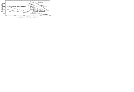
FIG. 1.: Energy parameter $\beta_{E}$ for the hexagonal lattice along $H_{c2}(t)$ line presented as a function of temperature: dashed line — the contribution of the first term in Eq. (24) with $m_{1}=m_{2}=0$, solid line — the full sum. Insert: Contour plot of the parameter $a_{h}$ as a function of $t$ and $b$. Magnetic induction is normalized to produce ${\rm d}b/{\rm d}t=-1$ at $t=1$.