Luttinger liquid with asymmetric dispersion

Abstract

We present an extension of the Tomonaga-Luttinger model in which left and right-moving particles have different Fermi velocities. We derive expressions for one-particle Green’s functions, momentum-distributions, density of states, charge compressibility and conductivity as functions of both the velocity difference $\epsilon$ and the strength of the interaction $\beta$. This allows us to identify a novel restricted region in the parameter space in which the system keeps the main features of a Luttinger liquid but with an unusual behavior of the density of states and the static charge compressibility $\kappa$. In particular $\kappa$ diverges on the boundary of the restricted region, indicating the occurrence of a phase transition.

In the last years there has been much interest in the study of one-dimensional (1D) condensed matter problems Reviews . Specific examples of experimentally realized 1D structures are: strongly anisotropic organic conductors organic conductors , charge transfer salts salts , quantum wires quantum wires , edge states in a two-dimensional (2D) electron system in the fractional quantum Hall (FQH) regime FQH and the recently built Carbon Nanotubes CNT . All these systems are no longer described by the usual 3D-like Fermi liquid picture. They are believed to belong to a novel, highly correlated state of matter known as the Luttinger liquid (LL) LL . Very recently, possible LL behavior in 2D high temperature superconductors has also been reported Orgad .

From the theoretical point of view the most widely studied 1D model is the so-called “g-ology” model Solyom , which is known to display the LL behavior characterized by spin-charge separation and by non-universal (interaction dependent) power-law correlation functions. In particular it predicts a momentum distribution function that vanishes at $p_{F}$ as $n(p)\sim(p-p_{F})^{2\gamma}$, where $\gamma$ is related to the strength of the electron-electron interaction (in the free case one has $\gamma=0$ and $n(p)\sim\theta(p_{F}+p)$). One of the simplest and yet very useful version of the “g-ology” model is the exactly solvable Tomonaga-Luttinger (TL) model, which describes left and right-moving electrons subjected to forward-scattering interactions TL .

In this Letter we propose a simple modification of the TL model in which left and right-moving electrons have different Fermi velocities $v_{L}$ and $v_{R}$. Previous studies of LL systems involving more than one Fermi velocity are related to an special class of chiral LL HC and to multiband and multichain models multi . Another interesting problem in which one has different values for $v_{F}$ is the interaction between parallel conductors leading to the so called Coulomb drag drag . We want to stress that the model we shall study is crucially different from all these systems since it is neither a purely chiral LL nor a multiband system with symmetric dispersion. Our theory is formally similar to a recently proposed model for the study of spin-orbit coupling in interacting quasi-1D systems spin-orbit . These authors, however, concentrated their attention on the interplay between velocity asymmetry and spin degrees of freedom, whereas here we derive and analyze physical consequences connected to the asymmetric dispersion only. As we shall see, this point of view allows us to obtain some novel non trivial features of the system.

To be specific we start by considering an asymmetric dispersion described by the following Hamiltonian

$$H=-i\hbar\int dx\,(v_{R}\psi^{\dagger}_{R}\partial_{x}\psi_{R}-v_{L}\psi^{\dagger}_{L}\partial_{x}\psi_{L})\\ +\pi U\int dx\,\psi^{\dagger}_{R}\,\psi_{R}\,\psi^{\dagger}_{L}\,\psi_{L},$$ (1)

where $\psi_{R,L}$ and $\psi^{\dagger}_{R,L}$ are the electron operators and $U$ is the strength of the forward-scattering electron-electron interaction. In the “g-ology” language we have $g_{2}=\pi\,U$ and $g_{4}=0$. The extension of our results to the general case ($g_{4}\neq 0$) is straightforward, here we consider this particular case in order to keep the discussion as clear as possible. We will set $\hbar=1$ from now on. Please note that both $v_{L}$ and $v_{R}$ are positive, and $U>0$ corresponds to repulsive interactions. This is the case we shall examine throughout this work.

Since the edge states of FQH systems have been successfully described in terms of chiral fermions with drift velocities proportional to $E/B$ FQH ($B$ is the uniform transverse magnetic field and $E$ is an electric field that keeps electrons inside the sample Fradkin ), the model above could be experimentally realized by putting together the edges of two FQH samples in the presence of different fields such that the resulting fractions are also different. In such experimental array $U$ represents the strength of the interaction between the charge-densities (CD) of each fermionic branch. Recent experiments on tunneling between edge states of laterally separated quantum Hall effect systems exp seems to indicate that the experiment we propose is indeed feasible.

One interesting result of this Letter is the appearance, due to the velocity asymmetry, of a new available region in the space of couplings in which the model (1) predicts an anisotropic phase, in the sense that the collective charge-density modes associated to each branch propagate in the same direction. However one has to be cautious with this prediction since our computations show that (1) is no longer valid in this region. Indeed, as we shall see, if we define

$$v_{0}=(v_{R}+v_{L})/2$$ (2)

and

$$\epsilon=\frac{v_{R}-v_{L}}{v_{R}+v_{L}},\qquad\beta=U/2v_{0},$$ (3)

we can only trust our model inside the unit circle in the $\epsilon-\beta$ parameter space ($\epsilon^{2}+\beta^{2}=1$). We then first explore the physics described by (1) in the restricted region. We shall be specially interested in discussing the cases of constant asymmetry ($\epsilon$ fixed) and constant interbranch interaction ($\beta$ fixed). In so doing we found a drastic change in the behavior of the charge compressibility $\kappa$ where the value at zero asymmetry is multiplied by a factor which diverges on the transition curve. Studied as a function of $\beta$ for fixed $\epsilon$, it first reaches a minimum and then there is a strong enhancement as $\beta\rightarrow\beta_{0}\equiv\sqrt{v_{R}v_{L}}/v_{0}$, in opposition to the monotonous decay present in the $\epsilon=0$ case. A similar change of behavior is present in the density of states (DOS) function. For $\beta$ and $\epsilon$ sufficiently small one recovers an ordinary LL system ($v_{0}\rightarrow v_{F}$,$v_{-}\rightarrow-v_{+}$).

Outside the restricted region there is a change in the sign of one of the “plasmon” velocities, accompanied by a dramatic change in the behavior of the Green function for that branch, which now diverges at long distances. This, together with the fact that $\kappa$ becomes negative, bring out that the model suffers some kind of instability in this region. It is important to stress that this region is absent for $v_{R}=v_{L}$.

We have studied the system (1) by using functional bosonization techniques FuncBos . This amounts to defining fermionic field operators in the Heisenberg picture. We then have a field-theoretical, Lagrangian formulation of the model. This, in turn, allowed us to obtain an action describing the dynamics of the bosonic collective excitations of the system. Using this action one can easily compute the dispersion relations for the CD oscillations. For short-range, constant electron-electron potentials, these dispersions are linear, with velocities given by $v_{\pm}=v_{0}\eta_{\pm}$, and

$$\eta_{\pm}=\epsilon\pm\sqrt{1-\beta^{2}}.$$ (4)

From this equation one sees that the propagation of the collective modes takes place for $\beta<1$. It becomes apparent that, in contrast to the usual answer for a TL model with $v_{R}=v_{L}$ and $g_{4}=0$, here one has two different velocities $v_{+}$ and $v_{-}$ for the propagation of left and right CD modes. Moreover, one of the velocities $v_{+}$ or $v_{-}$ goes to zero as the interaction and the asymmetry approach the curve $\epsilon^{2}+\beta^{2}=1$ and changes its sign beyond that curve, as anticipated above. If one keeps $\beta$ fixed this change of sign occurs for $\epsilon=\epsilon_{0}\equiv\sqrt{1-\beta^{2}}$. At this point, as we will see, there is a divergence in the charge compressibility and in the DOS, which suggests that a phase transition takes place.

Now, in order to get an insight into the physical consequences of the velocity difference, we compute single-particle quantities: the Green function $G_{r}(x,t)=\left\langle\psi_{r}(x,\tau)\psi^{\dagger}_{r}(0,0)\right\rangle_{\tau\rightarrow it}$ with $r=+\,(R),-\,(L)$, the momentum distribution function, the spectral function $\rho_{r}(q,\omega)$ given by

$$\rho_{r}(q,\omega)=-\frac{1}{\pi}\operatorname{Im}G_{r}^{\text{(ret)}}(q,\omega),$$ (5)

and the DOS defined as

$$N(\omega)=\frac{1}{2\pi}\sum_{r}\int dq\,\rho_{r}(q,\omega).$$ (6)

In these equations, $G_{r}^{\text{(ret)}}(q,\omega)$ is the Fourier transform of the retarded Green function:

$$G_{r}^{\text{(ret)}}(x,t)=i\theta(t)\left\langle\left\{\psi_{r}(x,t),\psi^{\dagger}_{r}(0,0)\right\}\right\rangle.$$ (7)

For the normal phase ($\beta^{2}+\epsilon^{2}<1$), the Green function at $T=0$ is given by

$$G_{r}(x,t)=\frac{1}{2\pi\alpha}\left(\frac{\alpha}{\alpha-ir(x-v_{r}t)}\right)^{\gamma+1}\\ \times\left(\frac{\alpha}{\alpha+ir(x-v_{-r}t)}\right)^{\gamma}$$ (8)

where $\alpha$ is an ultraviolet cutoff. The constant $\gamma$ has the usual expression in terms of the stiffness constant $K$, $\gamma=(K+K^{-1}-2)/4$, but in this constant $v_{F}$ must be replaced by the average $v_{0}$:

$$K=\sqrt{\frac{v_{0}-U}{v_{0}+U}}=\sqrt{\frac{1-\beta}{1+\beta}}.$$ (9)

In the outer region ($\beta^{2}+\epsilon^{2}>1$), for $v_{R}>v_{L}$, we get

$$G_{R}(x,t)=\frac{1}{2\pi}\frac{\left[\alpha-i(x-v_{-}t)\right]^{\gamma}}{\left[\alpha-i(x-v_{+}t)\right]^{\gamma+1}}$$ (10)

and

$$G_{L}(x,t)=\frac{-1}{2\pi\alpha^{2}}\frac{\left[\alpha-i(x-v_{-}t)\right]^{\gamma+1}}{\left[\alpha-i(x-v_{+}t)\right]^{\gamma}}.$$ (11)

From these results one obtains a momentum distribution of the Fermi type for the right branch, i.e., $n_{R}(p)\sim\theta(p-p_{R})$. However, the situation is very different for $n_{L}$. Indeed, when taking the appropriate $t\rightarrow 0^{-}$ limit in order to employ the usual definition of $n_{L}(p)$, one finds that the correlator increases linearly with distance, instead of having the $x^{-1}$ decay (typical of 3D-like systems) as is the case for the right branch, or the $x^{-(2\gamma+1)}$ behavior that yields the LL result in the “normal” LL region. This leads to $n_{L}\sim\delta^{\prime}(p+p_{L})$. The appearance of this divergent (at long distances) left correlator, together with a momentum distribution which is not a positive definite quantity, are clear indications that the model given by (1) is unphysical beyond $\beta^{2}+\epsilon^{2}=1$. (For $v_{L}>v_{R}$ the corresponding left and right behaviors are exchanged). We then conclude that the model given by (1) yields sensible results for $\epsilon^{2}+\beta^{2}<1$ and from now on we will restrict our study to that region.

From equation (5) one can calculate the spectral function $\rho_{r}(q,\omega)$. We obtain, as in the symmetric case, only one singularity in the positive frequency sector and one in the negative sector, as expected for spinless systems. The function diverges at those points as

$$\rho_{r}(q,\omega)\sim(\omega-v_{r}q)^{\gamma-1}(\omega-v_{-r}q)^{\gamma}\\ \times[\theta(\omega-v_{-}q)\theta(\omega-v_{+}q)+\theta(v_{-}q-\omega)\theta(v_{+}q-\omega)].$$ (12)

The exponents do not depend on $\epsilon$ whereas the position of the singularities does.

Concerning the DOS we get

$$N(\omega)=N_{0}(\omega)\left(1-\frac{\epsilon^{2}}{\epsilon_{0}^{2}}\right)^{-1-\gamma}$$ (13)

with

$$N_{0}(\omega)=\frac{1}{\pi v_{0}}\frac{(\omega/\omega_{0})^{2\gamma}}{\Gamma(2\gamma+1)(1-\beta^{2})^{\gamma+1/2}},$$ (14)

where $\omega_{0}=v_{0}/\alpha$ and $\Gamma$ is the Gamma function. We see that as the asymmetry is increased, the DOS grows from its value at $\epsilon=0$, and diverges at the point $\epsilon=\epsilon_{0}$. We want to stress that in systems with several spectral branches as multicomponent Tomonaga-Luttinger model Reviews and spin-polarized Luttinger liquids kimura a growing of the DOS as increasing the velocity difference between spectral branches is also observed. This disagrees with the result obtained in the system with spin-orbit coupling spin-orbit .

Using standard linear response theory one can express the conductivity as an integral of the retarded current density correlation function. At this point one has to recall that the naive definition of the current $j=v_{R}\rho_{R}-v_{L}\rho_{L}$ does not satisfy the continuity equation Giamarchi . This choice for $j$ leads to a frequency-dependent conductivity that diverges on the unit circle $\epsilon^{2}+\beta^{2}=1$ and becomes negative for $\epsilon^{2}+\beta^{2}>1$. However, as shown in Giamarchi it is indeed possible to build a physical current starting from the continuity equation. Extending this procedure for the present $\epsilon\neq 0$ case we obtain $j_{phys}=(1-\beta)(\rho_{R}-\rho_{L})+v_{0}\epsilon(\rho_{R}+\rho_{L})$. Using this expression we were able to get the frequency-dependent conductivity $\sigma$ as:

$$\sigma(\omega)=\frac{v_{0}\,(1-\beta)}{\pi\,\omega},$$ (15)

which is independent of $\epsilon$.

Let us now consider the static charge compressibility of this system, defined as $\kappa=\left\langle(\rho_{R}+\rho_{L})(\rho_{R}+\rho_{L})\right\rangle(q,\omega)$ for $\omega\rightarrow 0$. A straightforward computation yields

$$\kappa=\kappa_{0}\,\left(1-\frac{\epsilon^{2}}{\epsilon_{0}^{2}}\right)^{-1}$$ (16)

with

$$\kappa_{0}=\frac{1}{\pi\,v_{0}\,(1+\beta)},$$ (17)

where one sees the divergence that takes place, at fixed $\beta$, for $\epsilon=\epsilon_{0}$. This is similar to the behavior of the DOS, although both functions diverge with different exponents. Note that beyond $\epsilon_{0}$ one obtains negative values for the compressibility, a further indication that the model is not valid in that region. In Figure 1 we show the dependence of $\kappa$ on $\epsilon$ for different values of $\beta$. We see that the asymmetry enhances the compressibility. Of course, it is also possible to study $\kappa$ as function of the coupling $\beta$, for a fixed asymmetry. This is depicted in Figure 2 where one sees that in drastic departure from the symmetric case, which displays decreasing $\kappa$ for increasing $\beta$, now $\kappa$ reaches a minimum and then grows without bound as $\beta\rightarrow\beta_{0}$.

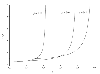
Figure 1: Static charge compressibility as function of $\epsilon$, for $\beta=0.1,0.6,0.9$.

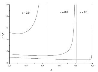
Figure 2: : Static charge compressibility as function of $\beta$, for $\epsilon=0.1,0.6,0.9$.

The critical behaviour of the static charge compressibility and the DOS at $\epsilon_{0}$ together with the “freezing” of one of the spectral branches ($v_{+/-}\rightarrow 0$) is an indication that a phase transition involving CD degrees of freedom takes place on the boundary $\beta^{2}+\epsilon^{2}=1$. A similar transition related to spin variables was also found in spin-orbit .

In summary, we have presented a simple modification of the usual TL model, in which left and right-moving particles have different Fermi velocities. By using functional bosonization methods we computed the dispersion relations of the underlying bosonic collective modes of the system. We showed that the velocity asymmetry gives rise to some remarkable features. We have found that the values for the electron-electron coupling $\beta$ and the asymmetry $\epsilon$ are restricted to lie inside the circumference $\epsilon^{2}+\beta^{2}=1$ in order to guarantee the stability of the LL described by (1). In this region, the DOS $N(\omega$) and the static charge compressibility $\kappa$ display a big deviation from the standard LL behavior. For a fixed asymmetry one sees that now $\kappa$ reaches a minimum and then grows without bound as $\beta\rightarrow\beta_{0}$. On the boundary of the restricted region the velocity of one spectral branch goes to zero. Also $\kappa$ and DOS diverge when approaching this critical boundary, indicating the appearance of a new phase.

To conclude we would like to stress that the idealized model we present here could be approximately realized by allowing the interaction between the edge states of two FQH plates. Since the drift velocities of the corresponding chiral LL’s are proportional to $E/B$, one could have $v_{R}\neq v_{L}$ by conveniently tuning up the corresponding values of these fractions.

- (1) J. Voit, Rep. on Prog. in Phys. 58, 977 (1995); H. J. Schulz, G. Cuniberti and P. Pieri, cond-mat/9807366; S. Rao and D. Sen, cond-mat/0005492; C. M. Varma, Z. Nussinov and Wim van Saarloos, cond-mat/0103393.
- (2) D. Jerome, H. Schulz, Adv. Phys. 31, 299 (1982).
- (3) A.J. Epstein et al., Phys. Rev. Lett. 47, 741 (1981).
- (4) A. R. Goni et al., Phys. Rev. Lett. 67, 3298 (1991).
- (5) X. G. Wen, Phys. Rev. Lett. 64 2206 (1990); Phys. Rev. B 41 12838 (1990); Int. Journal Mod. Phys. B 6 1711 (1992).
- (6) M. Bockrath, D. H. Cobden, J. Lu, A. G. Rinzler, R. E. Smalley, L. Balents, P. L. Mc-Euen, Nature 397 598 (1999); Z. Yao, H. W. J. Postma, L. Balents, C. Dekker, Nature 402 273 (1999).
- (7) F. D. M. Haldane, J. Phys. C 14, 2585, (1981).
- (8) D. Orgad et al., Phys. Rev. Lett. 86, 4362, (2001).
- (9) J. Solyom, Adv. Phys. 28, 209 (1979).
- (10) S. Tomonaga, Prog. Theor. Phys. 5 544 (1950); J. Luttinger, J. Math. Phys. 4 1154 (1963); D. Mattis and E. Lieb, J. Math. Phys. 6 304 (1965).
- (11) A. F. Ho and P. Coleman, Phys. Rev. Lett. 83, 1383, (1999); Phys. Rev. B 62, 1688, (2000).
- (12) C. M. Varma and A. Zawadowski, Phys. Rev. B 32, 7399, (1985); K. Penc and J. Solyom, Phys. Rev. B 41, 704, (1990); L. Balents and M. P. A. Fisher, Phys. Rev. B 53, 12133, (1996).
- (13) K. Flensberg, Phys. Rev. Lett. 81, 184, (1998); Y. V. Nazarov and D. V. Averin, Phys. Rev. Lett. 81, 653, (1998).
- (14) A. V. Moroz, K. V. Samokhin and C. H. W. Barnes, Phys. Rev. Lett. 84, 4164, (2000); Phys. Rev. B 62, 16900, (2000).
- (15) Eduardo Fradkin, Field Theories of Condensed Matter Systems, Addison-Wesley Publishing Co., 1991.
- (16) W. Kang, H. L. Stormer, L. N. Pfeiffer, K. W. Baldwin, K. W. West, Nature 403, 59 (2000).
- (17) H. C. Fogebdy, J. of Phys. C 9, 3757, (1976); D.Lee and Y.Chen, J. of Phys. A 21, 4155 (1988); C.M.Naón, M.C.von Reichenbach and M.L.Trobo, Nucl.Phys.[FS] B435 567 (1995); A. Iucci, C. Naón, Phys. Rev. B 61, 15530 (2000), cond-mat/9912193; V. Fernández and C. Naón, Phys. Rev. B 64, 033402, (2001).
- (18) T. Kimura, K. Kuroki, and H. Aoki, Phys. Rev. B 53, 9572, (1996).
- (19) T. Giamarchi, Phys. Rev. B 44, 2905, (1991).