Nonequilibrium coupled Brownian phase oscillators

Abstract

A model of globally coupled phase oscillators under equilibrium (driven by Gaussian white noise) and nonequilibrium (driven by symmetric dichotomic fluctuations) is studied. For the equilibrium system, the mean-field state equation takes a simple form and the stability of its solution is examined in the full space of order parameters. For the nonequilbrium system, various asymptotic regimes are obtained in a closed analytical form. In a general case, the corresponding master equations are solved numerically. Moreover, the Monte-Carlo simulations of the coupled set of Langevin equations of motion is performed. The phase diagram of the nonequilibrium system is presented. For the long time limit, we have found four regimes. Three of them can be obtained from the mean-field theory. One of them, the oscillating regime, cannot be predicted by the mean-field method and has been detected in the Monte-Carlo numerical experiments.

PACS numbers: 05.40.-a, 05.60.-k

I Introduction

A system of coupled oscillators has been treated as a model system of collective dynamics that exhibits a plenty of interesting properties such as equilibrium and nonequilibrium phase transitions, coherence, synchronization, segregation and clustering phenomena. It has been used to study active rotator systems shin , electric circuits, Josephson junction arrays wies , charge-density waves stro oscillating chemical reactions kura , planar XY spin models aren , networks of complex biological systems such as nerve and heart cells win .

Such a system of N-coupled phase oscillators is determined by a set of equations of motion in the form mur

$$\dot{x}_{i}=\omega_{i}+f(x_{i})+\sum_{j=1}^{N}K_{ij}G(x_{j},x_{i})+\eta_{i}(t),$$

$$i=1,...,N,$$ (1)

where $x_{i}$ denotes the phase of the $i$th oscillator and $\omega_{i}$ is its local frequency, i.e. its frequency in the absence of the interaction between the oscillators. The local force is represented by the function $f(x)$ and $G(x,y)$ includes the coupling effect between oscillators. The constants $K_{ij}$ are the coupling strengths and $\eta_{i}(t)$ characterizes fluctuations in the system. In the case of weak coupling, $G(x,y)=G(x-y)$ and $G$ is a periodic function of its argument. The specific model $G(x)=\sin x$ has been intensively studied and in the physical literature it is known as a Kuramoto model kura . If $K_{ij}$ are positive then the coupling is excitatory (meaning $x_{i}$ tends to pull $x_{j}$ toward its value). If $K_{ij}$ are negative then the coupling is inhibitory (it tends to increase the difference between $x_{i}$ and $x_{j}$). Most of studies of the model focus on the global coupling (each oscillator interacts with all the other oscillators), where all pairs are interacting with uniform strength, $K_{ij}=K/N$. Then the mean-field treatment holds exactly when $N\to\infty$.

In the paper we study a special case of the model (I) when the fluctuation term represents thermal-equilibrium and nonequilibrium fluctuations. The remainder of this paper is organized as follows. In the next section we analyze an equilibrium system. It is a model with thermal fluctuations being Gaussian white noise. In Sec. III, we study a nonequilibrium system by adding the second fluctuation source, i.e., a zero-mean, exponentially correlated symmetric two-state Markov process. It can describe a case when local frequencies $\omega_{i}$ of the oscillators fluctuate in time. In Sec. III.2, we present the mean-field numerical solutions of a corresponding master equation and discuss results of the Monte Carlo simulations of Langevin equations. Finally, in Sec. IV we formulate the main conclusions.

II Mean-field equilibrium system

In this section, we analyze a system of phase oscillators in contact with thermostat of temperature $T$, namely,

$$\dot{x}_{i}=-\sin x_{i}+\frac{K}{N}\sum_{j=1}^{N}\sin(x_{j}-x_{i})+\Gamma_{i}(t),$$

$$i=1,...,N,$$ (2)

where thermal-equilibrium fluctuations $\Gamma_{i}(t)$ are modeled by zero-mean delta-correlated Gaussian white noise,

$$\langle\Gamma_{i}(t)\rangle=0,\quad\langle{\Gamma}_{i}({t}){\Gamma}_{j}({s})\rangle=2T\delta_{ij}\delta({t}-{s}).$$ (3)

This model can represent a planar model with anisotropy or external field. More general models than (II) has been analyzed. Nevertheless, we reconsider the simplified model (II) because of two reasons. Firstly, the state equation of the system has a simple tractable form. Secondly, a new aspect of the stability problem of states is presented.

Let us rewrite the interaction term in the form rei1

$$\frac{1}{N}\sum_{j=1}^{N}\sin(x_{j}-x_{i})=s\cos x_{i}-c\sin x_{i},$$ (4)

where the averages

$$s=\frac{1}{N}\sum_{j=1}^{N}\sin x_{j},\quad c=\frac{1}{N}\sum_{j=1}^{N}\cos x_{j}$$ (5)

are order parameters for the system (I). In the thermodynamical limit, $N\to\infty$, for each oscillator $x_{i}=x$ the mean-field Langevin equation is obtained from the system (I) and reads

$$\dot{x}=F(x,s,c)+\Gamma(t),$$ (6)

where the effective force $F(x,s,c)=-V^{\prime}(x,s,c)$ (the prime denotes a differentiation with respect to $x$) and the effective potential

$$V(x,s,c)=-(1+Kc)\cos x-Ks\sin x.$$ (7)

Let us introduce a probability density

$${\hat{P}}(x,t)=\langle\delta\left(x(t)-x\right)\rangle$$ (8)

of the process (6), where $x(t)$ is a solution of (6) for a fixed realization of noise $\Gamma(t)$ and $\langle...\rangle$ denotes an average over all realizations of $\Gamma(t)$. This density is normalized on a real axis,

$$\int\limits_{-\infty}^{\infty}{\hat{P}}(x,t)\;dx=1$$ (9)

and obeys the Fokker-Planck equation

$$\frac{\partial{\hat{P}}(x,t)}{\partial t}=\frac{\partial}{\partial x}V^{\prime}(x,s,c){\hat{P}}(x,t)+T\frac{\partial^{2}}{\partial x^{2}}{\hat{P}}(x,t).$$ (10)

The reduced probability density $P(x,t)$ defined by the relation

$$P(x,t)=\sum\limits_{n=-\infty}^{\infty}{\hat{P}}(x+2\pi n,t)$$ (11)

satisfies the Fokker-Planck equation (10) as well, is periodic

$$P(x+2\pi n,t)=P(x,t)\enskip\mbox{for any integer}\ n$$ (12)

and normalized on one period,

$$\int\limits_{x_{0}}^{x_{0}+2\pi}P(x,t)\;dx=1\enskip\mbox{for any real}\ x_{0}.$$ (13)

The order parameters $s$ and $c$ are determined self-consistently from the set of two equations kim ,

$$s=\langle\sin x\rangle = \int\limits_{-\infty}^{\infty}\sin x{\hat{P}}(x,t)\;dx$$ (14)

$$= \int\limits_{0}^{2\pi}\sin xP(x,t)\;dx\equiv g(s,c),$$

$$c=\langle\cos x\rangle = \int\limits_{-\infty}^{\infty}\cos x{\hat{P}}(x,t)\;dx$$ (15)

$$= \int\limits_{0}^{2\pi}\cos xP(x,t)\;dx\equiv h(s,c),$$

where ${\hat{P}}(x,t)\equiv{\hat{P}}(x,s,c,t)$ and $P(x,t)\equiv P(x,s,c,t)$ depend on parameters $s$ and $c$ via the effective one-particle potential $V(x,s,c)$ given by (7).

Our concern is the behavior of the system in the limit of long time, $t\to\infty$. The stationary state is a thermodynamic equilibrium state and the stationary solution $P_{st}(x)$ of (10) is a Gibbs distribution,

$$P_{st}(x)=N\mbox{e}^{-V(x,s,c)/T},$$ (16)

$$N^{-1}=\int\limits_{0}^{2\pi}\mbox{e}^{-V(x,s,c)/T}\;dx.$$ (17)

It is well known that in the equilibrium state the average angular velocity vanishes (the principle of detailed balance holds) $\langle\dot{x}\rangle=0$ (see, e.g., luczA ). Then from (6) it follows that

$$s=\langle\sin x\rangle=0$$ (18)

in the stationary state and only a symmetric state is realized for which the effective potential reduces to the simple form

$$V(x,s,c)=V(x,0,c)=-(1+Kc)\cos x.$$ (19)

The form of this potential is the same as for a system of non-interacting oscillators, $V(x)=-\cos x$. However, the amplitude $A=1+Kc$ can change. If $c>0$ then the coherence effect occurs and the most probable state is the deterministic state $x=0$. On the other hand, if $1+Kc<0$ then the most probable state changes and the new state is $x=\pi$.

Figure 1: The order parameter $c=\langle\cos x\rangle$ for the system of coupled phase oscillators in equilibrium as a function of the coupling strength $K$ and temperature $T$. All data have been obtained as solutions of the implicit equation (20). The upper plot shows the dependence of $c$ on the coupling $K$ for selected temperatures. Even at $T=0$ the equation (20) has three solutions $c=(c_{1},c_{2},c_{3})=(1,-1,-1/K)$ for $K>1$ (for $K<1$ there exists only one solution $c_{1}=1$). The lower plot shows the order parameter $c$ as a function of temperature. As it could be expected, for large thermal fluctuations, stochastic forces overwhelm the potential and the coupling, and the solution tends to $c_{1}=0$ as $T\to\infty$. The stability analysis shows that stable are only solutions with $c>0$.

Figure 2: The plot shows a vector field of the right hand side of the dynamical system (26)-(27) for $K=3.1$ and $T=0.5$. Three black dots are solutions of the mean-field problem, i.e. stationary points of (26)-(27). The upper solution $c_{1}$ is a stable node, the middle one $c_{3}$ is an unstable node and the lowest one $c_{2}$ is a saddle point. Let us notice that stability analysis in one dimension (assuming that $s=0$) would lead to a false conclusion that the lowest point $c_{2}$ is stable. Solid lines are a result of the Monte Carlo simulation of $8000$ particles with the initial condition set to the mean-field solutions $c_{2}$ and $c_{3}$. In the $(s,c)$-space the system evolves along the clockwise or anticlockwise “semicircles” (depending on the initial microstate) to the stable node $(0,c_{1})$.

The order parameter $c$ is determined by the equation

$$cI_{0}\left(\frac{1+Kc}{T}\right)=I_{1}\left(\frac{1+Kc}{T}\right),$$ (20)

where $I_{0}(z)$ and $I_{1}(z)$ are the modified Bessel functions. This equation can possess one, two or three solutions (see Fig. 1). If the coupling strength $K<1$ then only one solution exists for any temperature $T$ of the system (Fig. 1a). For high temperature, $T>>1$, the upper branch $c_{1}$ tends to zero as $c\sim T^{-1}$ (Fig. 1b). The opposite asymptotics, when $T\to 0$, can be obtained as well. In this case the upper branch $c_{1}\to 1$ for any $K>0$. The lower branch $c_{2}\to-1$ and the middle branch $c_{3}\to-1/K$ for $K>1$ (Fig. 1a). Now, let us study stability of the stationary solutions. The linear stability analysis should be performed on the full set of equations of motion for average values $s$ and $c$, (14) and (15). Multiplication of (10) by either $\sin x$ or $\cos x$ and integration over $x$ gives

$$\dot{s} = -(1+K\,c)\,<sc>\,+\,T\,s\,+\,K\,s\,<c^{2}>,$$ (21)

$$\dot{c} = (1+K\,c)\,<s^{2}>\,-\,T\,c-\,K\,s\,<sc>,$$ (22)

and $<...>$ stands for the averages of products of $\cos x$ and/or $\sin x$ (e.g. $<sc>=<\sin x\cos x>$). To make the system (21)-(22) closed, we should write equations of motion for the unknown statistical moments $<sc>$, $<s^{2}>$ and $<c^{2}>$. New, higher-order moments will occur and in this way we obtain a hierarchy of infinite number of differential equations for moments, which is difficult to handle. Therefore we proceed in another way. Let us notice that for $<s^{2}>\equiv<\sin^{2}x>$ one may write $<s^{2}>=1-<\cos^{2}x>=1-<c^{2}>$. Additionally, one can introduce deviations from the mean values and write $<c^{2}>=c^{2}+<(\delta c)^{2}>$ as well as $<sc>=s\,c+<\delta s\delta c>$. As a result, one obtains

$$\dot{s}=-(c-K\,<(\delta c)^{2}>-T)\,s$$

$$-(1+K\,c)\,<\delta s\delta c>,$$ (23)

$$\dot{c}=(1+K\,c)\,(1-c^{2}-<(\delta c)^{2}>)-T\,c-K\,s^{2}\,c$$

$$-K\,s\,<\delta s\delta c>.$$ (24)

From (18) we know that $s=0$ is a stationary solution of the above equations. In order to obtain this solution $s=0$ from (II), the correlator $<\delta s\delta c>$ should vanish in the stationary limit, i.e., $<\delta s\delta c>\to 0$ as $t\to\infty$. Insertion of $s=0$ into the second equation (II) with $\dot{c}=0$ yields stationary solutions for $c$. They are determined by the equation

$$(1+Kc)\,(1-c^{2}-<(\delta c)^{2}>)-Tc=0$$ (25)

These solutions depend on the unknown variance $<(\delta c)^{2}>$. In the low temperature limit $T\to 0$, the variance $<(\delta c)^{2}>\to 0$ and we recover the solutions $c_{1}=1,c_{2}=-1$ and $c_{3}=-1/K$. In this case, the linear stability analysis of (II)-(II) shows that the stationary point $(0,c_{1})$ is a stable node, the point $(0,c_{2})$ is a saddle and the solution $(0,c_{3})$ is an unstable node. For $T>0$, the stability of solutions remains unchanged. Indeed, in our simulations we have confirmed this statement. We have also analyzed an auxiliary dynamical system defined by a set of two differential equations, namely (cf. (14) and (15)),

$$\dot{s}=-s+g(s,c),$$ (26)

$$\dot{c}=-c+h(s,c).$$ (27)

The stationary solution of this system is the same as the equilibrium state of the system (6). In Fig. 2 we present a vector field generated by the dynamical system (26)-(27) and its three stationary points $(s_{i},c_{i}),i=1,2,3$. One can infer that the upper point $(0,c_{1})$ is a stable node, the lower point $(0,c_{2})$ is a saddle and the middle point $(0,c_{3})$ is an unstable node (the same as for (II)-(II)). We have also found unexpectedly that the trajectory of the system (26)-(27) is the same as that obtained from simulations of the set of Langevin equations (II), see Fig. 2. It allows us to formulate the conjecture that the hierarchy of infinite number of equations for moments of the set $(\sin x,\cos x)$is equivalent to (26)-(27). Unfortunately, we cannot prove it rigorously.

III Mean-field nonequilibrium system

Nonequilibrium systems can be modeled by including a term which describes non-thermal and nonequilibrium fluctuations, noise and perturbations. There are many possibilities to do this but here we consider a slight modification of the previous model, namely,

$$\dot{x}_{i}=-\sin x_{i}+\frac{K}{N}\sum_{j=1}^{N}\sin(x_{j}-x_{i})+\Gamma_{i}(t)+\xi_{i}(t),$$

$$i=1,...,N,$$ (28)

The random functions $\xi_{i}(t)$ represent nonequilibrium fluctuations and are modeled by a symmetric dichotomic Markovian stochastic processes chem ,

$$\xi_{i}(t)=\{-a,a\},\mbox{ }a\mbox{ }>0,$$ (29)

$$P(-a\rightarrow a)=P(a\rightarrow-a)=\mu,$$

where $P(-a\rightarrow a)$ is a probability per unit time of the jump from the state $-a$ to the state $a$. This process is of zero average, $\langle\xi_{i}(t)\rangle=0$, and exponentially correlated,

$$\langle\xi_{i}(t)\xi_{j}(s)\rangle=a^{2}\delta_{ij}e^{-\left|t-s\right|/\tau},$$ (30)

where $\tau=1/2\mu$ is correlation time of the process $\xi_{i}(t)$. So, it is characterized by two parameters: its amplitude $a$ (or equivalently the variance $<\xi^{2}(t)>=a^{2}$) and the correlation time $\tau$.

The mean-field Langevin equation takes the form

$$\dot{x}=-V^{\prime}(x,s,c)+\Gamma(t)+\xi(t)$$ (31)

and the corresponding master equations read van

$$\frac{\partial P_{+}(x,t)}{\partial t}=\frac{\partial}{\partial x}\left[V^{\prime}(x,s,c)-a\right]P_{+}(x,t)$$

$$+T\frac{\partial^{2}}{\partial x^{2}}P_{+}(x,t)-\mu P_{+}(x,t)+\mu P_{-}(x,t)$$ (32)

$$\frac{\partial P_{-}(x,t)}{\partial t}=\frac{\partial}{\partial x}\left[V^{\prime}(x,s,c)+a\right]P_{-}(x,t)$$

$$+T\frac{\partial^{2}}{\partial x^{2}}P_{-}(x,t)+\mu P_{+}(x,t)-\mu P_{-}(x,t)$$ (33)

where the probability densities

$$P_{+}(x,t)\equiv P(x,a,t),\quad P_{-}(x,t)\equiv P(x,-a,t).$$ (34)

depend on the order parameters $s$ and $c$, which in turn depend self-consistently on the marginal density $P(x,t)=P_{+}(x,t)+P_{-}(x,t)$ via the relations (14)-(15). Eqs (III)-(III) cannot be solved analytically, even in the stationary state. However, in some limiting cases, stationary solutions of them are known, e.g., if the correlation time $\tau\to\infty$ (the adiabatic limit) or if temperature of the system is zero, $T=0$.

III.1 Analytical results

From the ratchet theory we know that the stationary average angular velocity is zero, $\langle v\rangle=\langle\dot{x}\rangle=0$, because the potential (7) is symmetric and fluctuations (29) are symmetric luczA . Therefore

$$s=\langle\sin x\rangle=0$$ (35)

and $V(x,s,c)$ takes the same form as in the previous case (19). In the adiabatic limit, the equation determining a stationary state is

$$c=\frac{1}{2}\int\limits_{0}^{2\pi}\cos x\;\left[p_{+}(x,c)+p_{-}(x,c)\right]dx,$$ (36)

where the stationary probability densities $p_{i}(x,c),\left(i=+,-\right)$ read

$$p_{i}(x,c)=\frac{U_{i}(x,c)\int\limits_{x}^{x+2\pi}U^{-1}_{i}(y,c)dy}{\int\limits_{0}^{2\pi}U_{i}(x,c)\int\limits_{x}^{x+2\pi}U^{-1}_{i}(y,c)dydx}$$ (37)

and

$$U_{\pm}(x,c)=\mbox{e}^{V(x,0,c)/T}\mbox{e}^{\pm ax/T}.$$ (38)

In the second limit, i.e. when temperature of the system is zero, $T=0$, the stationary state is determined by the equation

$$c=\frac{\int\limits_{\Omega(c)}\cos x\;D^{-1}(x,c)\mbox{e}^{-\Psi(x,c)}\;dx}{\int\limits_{\Omega(c)}D^{-1}(x,c)\mbox{e}^{-\Psi(x,c)}\;dx}.$$ (39)

where the thermodynamic potential

$$\Psi(x,c)=\int\limits_{0}^{x}D^{-1}(y,c)V^{\prime}(y,0,c)\;dy$$ (40)

and the effective diffusion function

$$D(x,c)=\tau\left[a^{2}-V^{\prime}(x,0,c)^{2}\right].$$ (41)

The integration interval $\Omega(c)=[0,2\pi]$ iff $D(x,c)>0$. If in some intervals the function $D(x,c)$ is negative then $\Omega(c)=[x_{1},x_{2}]$, where $x_{1}$ and $x_{2}$ are suitable roots of the equation $D(x,c)=0$ and in the interval $[x_{1},x_{2}]$ the diffusion function is positive.

The limiting case $T=0$ and $\tau\to\infty$ is analytically tractable. From the master equations it follows that in this case the stationary state is determined by the equation

$$\left[a^{2}-V^{\prime}(x,0,c)^{2}\right]P(x)=const.$$ (42)

In the diffusive regime, when dichotomic noise activates both forward and backward transitions over barriers of the effective potential, the solution of (42) is

$$P(x)=const./\left[a^{2}-V^{\prime}(x,0,c)^{2}\right]$$ (43)

and the only solution of the state equation (15) is $c=0$. In the non-diffusive regime, when dichotomic noise cannot activate neither forward nor backward transitions over barriers of the effective potential, the normalized solution of (42) has the form

$$P(x)=\frac{1}{2}\left[\delta(x-x_{1})+\delta(x-x_{2})\right]$$ (44)

where $x_{1}$ and $x_{2}$ are solutions of the equation

$$a^{2}-V^{\prime}(x,0,c)^{2}=0.$$ (45)

If $1+Kc>0$ then the state equation is determined by

$$c=\cos\left[\arcsin(a/(1+Kc))\right]$$ (46)

This equation can possess two positive roots, $c_{1}>c_{2}>0$. The solution $c_{1}$ is stable while $c_{2}$ is unstable. If $1+Kc<0$ then

$$c=-\cos\left[\arcsin(a/(1+Kc))\right].$$ (47)

This equation can possess two negative roots which are unstable. It is depicted in Fig. 3.

III.2 Numerical methods

In a general case the mean-field problem reduces to the set of non-linear master equations (III) and (III) which has to be solved. Apart of a few previously considered special cases which can be treated analytically, only numerical methods are applicable. We have approached the numerical problem of solving (III) and (III) as follows. Conditions of self-consistency have been considered (14) and (15) as the non-linear minimization problem in two dimensions on the bounded domain $-1\leq s\leq 1$ and $-1\leq c\leq 1$. It has been handled in a standard way, making use of numerical libraries. However, each evaluation of functions $g$ and $h$ for given $(s,c)$ requires the knowledge of stationary solution of the system (III), (III) with fixed $s$ and $c$. This is, in turn, a linear boundary value problem which can be easily solved with the help of finite element method (FEM). In the case $T=0$, the stationary distribution $P(x)$ is given be quadratures but it is very difficult to handle it analytically. Moreover, we found it practically easier to obtain a FEM solution for small enough $T$ then to estimate, divergent in some cases, triple integrals.

Additionally, in order to verify mean-field results we have performed Monte-Carlo simulations of the Langevin equations (III). This, independent method enabled not only verification of numerical results but also applicability of the mean-field approach. Because the Monte-Carlo simulation follows the evolution of microscopic state of the system it can be considered as a numerical experiment, in contrary to the mean-field approach which is only an approximation. In general, Monte-Carlo simulations of globally interacting $N$-particles require $\simeq N^{2}$ operations per time step. The special form of the interaction term $\simeq\sin(x_{j}-x_{i})$, leads to relations (4) and (5). In the course of simulation the average values $s$ and $c$ need to be evaluated only once per a simulation step, what reduces the number of operations per a time step to $\simeq N$.

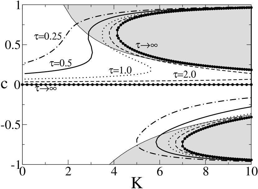
Figure 3: Solutions of the stationary mean-field problem (14),(15), (III) and (III). The temperature is zero and the amplitude of dichotomic fluctuations is $a=2.8$. As in the equilibrium case, negative solutions are unstable. Stable, and observed in Monte-Carlo simulations solutions lie in the upper plane $c>0$. Grey regions depict places where the locking condition is met i.e. maximum of the effective force overwhelms the amplitude of fluctuations. One can notice that for small values of $\tau$, the system starts to behave as an equilibrium one. In the case $\tau\to\infty$ the asymptotic analytical solution is shown. For finite $\tau$ numerical results are depicted. In this case the system exhibits onset of hysteresis in $c(K)$.

III.3 General case: numerical analysis

All numerical mean-field results have been obtained in the stationary regime. First we study the zero-temperature case, $T=0$. The natural characteristics of the stationary state are statistical moments, in particular the first two moments $<x>$ and $<x^{2}>$. These moments are not good characteristics in the case considered. If the system is spatially periodic, then for any spatially periodic function $A(x)=A(x+2\pi)$ we can calculate its mean value exploiting either the probability density ${\hat{P}}(x,t)$ or the reduced probability distribution $P(x,t)$ because then the equality

$$\langle A(x)\rangle=\int\limits_{-\infty}^{\infty}A(x){\hat{P}}(x,t)\;dx=\int\limits_{0}^{2\pi}A(x)P(x,t)\;dx$$ (48)

holds. It is not a case for non-periodic functions and then there is a problem which the distribution should be used for calculationg the average value. Therefore we consider periodic functions. Here, two natural order parameters $s=<\sin x>$ and $c=<\cos x>$ occur which characterize the probability distribution in the same way as $<x>$ and $<x^{2}>$. Indeed, the function $\sin x$ is odd like the function $x$ and the function $\cos x$ is even like the function $x^{2}$. Because $<\sin x>=0$, below we analyze $<\cos x>$. In Fig. 3 we show the dependence of the order parameter $c=\langle\cos x\rangle$ on the coupling strength $K$. One can distinguish two main regimes: the diffusive (dichotomic noise activates transitions over barriers of the effective potential (19)) and non-diffusive or locked (dichotomic noise cannot activate transitions over barriers of the effective potential (19)). These two regimes, marked by white and gray regions in Fig. 3, are separated by two critical lines: $Kc+1=a$ for positive values of $c$ and $Kc+1=-a$ for negative values of $c$. For negative $c$, the dependence of $c$ upon $K$ is qualitatively the same as for the equilibrium system (Fig. 1). These solutions are unstable and therefore will not be considered. Now, let us discuss the positive solutions $c>0$. They depend strongly on the correlation time $\tau$ of dichotomic fluctuations. For short correlation time, the order parameter $c$ monotonically increases with the growing coupling $K$. For longer correlation time, new effects arise: the dependence is discontinuous and hysteretic. In some domain there are three solutions $c_{1}>c_{2}>c_{3}$. The solutions $c_{1}$ and $c_{3}$ are stable while $c_{2}$ is unstable. The hysteresis is bigger and bigger when $\tau$ increases. The jumping point $K_{1}$ from the lower to the upper branch tends to infinity and the jumping point $K_{2}$ from the upper to the lower branch tends to a constant value determined by eq. (46). The upper branch of solutions $c_{1}(K)\to 1$ and the lower branch $c_{3}(K)\to 0$ when $\tau\to\infty$. For $\tau=\infty$, the solutions split into two branches of three solutions, namely, one $c_{3}=0$ and two other determined by (46). The stationary mean-field solutions have been verified by the Monte-Carlo simulations. The comparison is presented in Fig. 4.

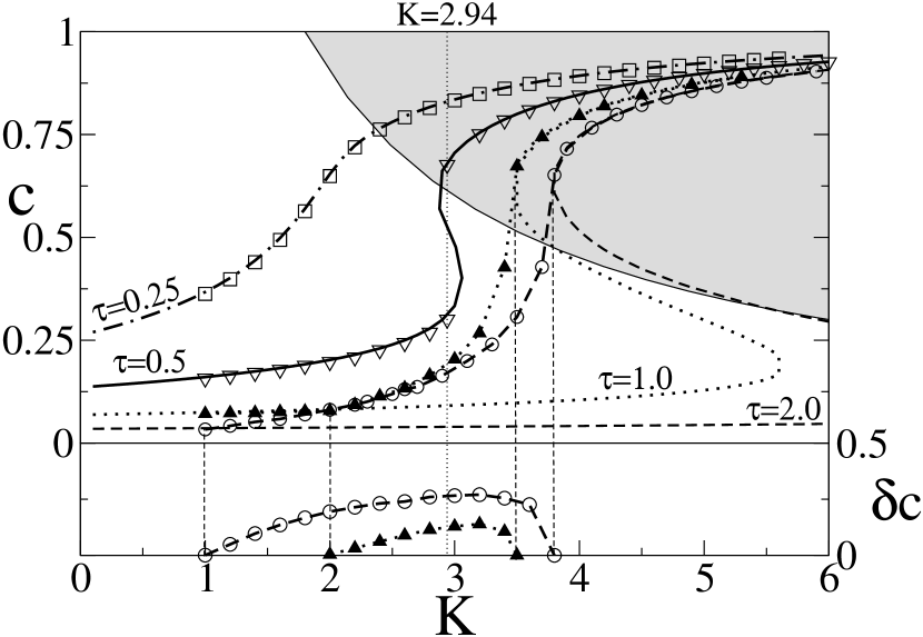
Figure 4: The same case as in Fig. 3: the comparison of mean-field results and Monte-Carlo simulations. For $\tau=0.25$ and $\tau=0.5$ there is a perfect agreement of the Monte Carlo and mean-field methods. However, for $\tau=1$ and $\tau=2$ temporal oscillations of density of particles appear in the Monte-Carlo method. Thus the order parameter also performs temporal oscillations. An averaged value of those oscillations differs from those coming from the mean-field solution. The standard deviation of $c$ (averaged in time) is shown in the lower insert. One can notice that if oscillations disappear ($\delta c=0$) then the simulated values of $c$ agree very well with mean-field predictions.

Simulations show that the implicit assumption of time-independent stationarity of the system (when $t\to\infty$) is restricted to some values of parameters of the model. Indeed, if the time-independent stationary state of the system exists then the mean-field solutions agree with simulations. In particular, for $\tau=0.5$ the hysteresis is observed (see point $K=2.94$ in Fig. 4 and Fig. 7). However, for longer correlation time $\tau$, temporarily oscillating steady-states exist for which the probability distribution $P(x,t)$ is periodic in time. In consequence the order parameters $s=s(t)$ and $c=c(t)$ are time-periodic and in the limit of long time, the time-dependent steady-states appear. This is the case when the mean-field predictions fail, e.g. the hysteresis is not realizable. In Fig 4 we depicted this phenomenon for $\tau=1,2$. We have noticed only monotonic dependence of $c$ upon $K$ (if $c$ is a periodic function of time, its time average is taken). The quantity which can characterize the time-independent stationarity/time-dependent stationarity (i.e. oscillations) of the long time state is the time-averaged standard deviation $\left(\delta c\right)^{2}=\langle c^{2}\rangle_{t}-\langle c\rangle_{t}^{2}$ of the order parameter. We have observed that if $\delta c=0$ then the mean-field solutions are correct. Otherwise, they are incorrect. It is shown in the lower insert of Fig. 4.

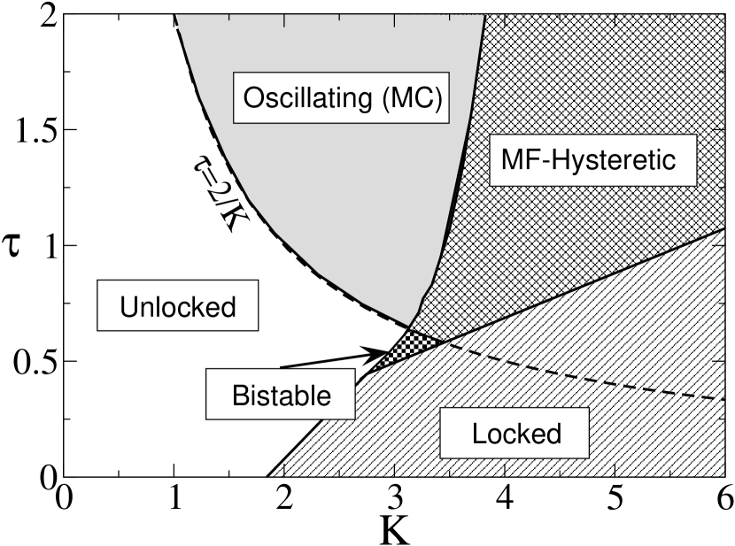
Figure 5: The phase diagram of the system with $a=2.8$ and $T=0$. Five various regimes are distinguished: unlocked and oscillating, mean-field hysteretic, locked and bistable. The oscillating regime has been verified by Monte-Carlo simulations. All other data come from the stationary mean-field problem. The empirical formula $\tau=2/K$ surprisingly well fits the left boundary of the oscillating region.

In Fig. 5 we present the phase diagram on the $\left(K,\tau\right)$ plane for a fixed amplitude $a=2.8$ of dichotomic fluctuations. In the case of non-interacting oscillators, this value of $a$ corresponds to the diffusive regime. Roughly speaking, there are two regions: diffusive when $a>1+Kc(\tau)$ (i.e. dichotomic noise can induce transitions over barriers of the effective potential (19)) and non-diffusive when $a<1+Kc(\tau)$ (i.e. dichotomic noise cannot induce transitions over barriers of the effective potential (19)). The diffusive region is divided into two parts which we call the unlocked regime (where the mean-field solutions are correct) and the oscillating regime (where the mean-field solutions fail). In the unlocked regime, there is one and only one time-independent stationary state and there is only one stationary value of the order parameter $c=<\cos x>$ which is always stable. In this regime, the reduced stationary probability density $P_{st}(x)\neq 0$ for any $x$. It means that with non-zero probability the phases of the oscillators can take any value of $x$ and oscillators are not synchronized. In the oscillating regime, the only stationary state is temporarily oscillating state for which $\lim_{t\to\infty}P(x,t)$ is time-periodic and the order parameter $c=c(t)$ is time-periodic. From previously discussed results it follows that this regime is bounded from the right, i.e. if $K>K_{0}$ then this regime disappears. The critical value $K_{0}$ can be determined by Eq. (46) from the condition that it possesses the double root $c_{1}=c_{2}$. The oscillating regime is presented in Fig. 6, where we show evolution of two distributions, the full density ${\hat{P}}(x,t)$ normalized on the interval $\left(-\infty,\infty\right)$ and the reduced density $P(x,t)$ normalized on one period. In the latter case, the density oscillates between the distribution of one maximum around $\pi$ (it corresponds to the maximum of the local potential $-\cos x)$ and the distribution of two maxima around $0$ and $2\pi$ (it corresponds to the minima of the local potential).

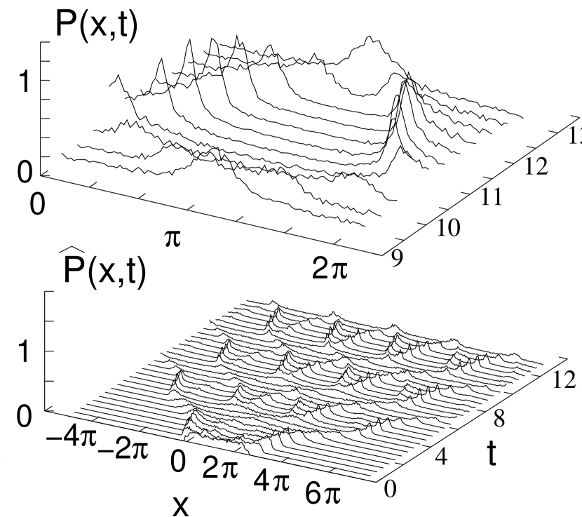
Figure 6: Monte Carlo simulations of the system for $a=2.8$, $\tau=1.0$, $K=2.94$ and $T=0$. None of the mean-field prediction is realized. The only stable solution is a stationary one. In the upper plot evolution of the probability density reduced to $x\in(0,2\pi)$ is shown. In lower plot the full distribution is presented. A starting value was a uniform distribution on $x\in(0,2\pi)$.

In turn, the non-diffusive region is divided into two other parts which we call the locked and hysteretic regimes. In the locked regime, only one steady-state solution exists. In this regime, there are intervals of $x$ for which the reduced stationary probability density $P_{st}(x)=0$ and the phases of the oscillators are locked in these intervals. It is an effect of interaction and corresponds to the synchronization of oscillators (let us remember that in the case on non-interacting oscillators, the diffusive regime is realized in which the phases can take arbitrary values). The synchronization is stronger if the support of $P_{st}(x)$ is smaller. In this regime, there is only one mean-field value of $c=<\cos x>$ which is always stable. The so-called MF hysteretic regime is defined in the following way: There are three mean-field stationary values $c_{1}>c_{2}>c_{3}>0$ of the order parameter. The solutions $c_{1}$ and $c_{3}$ are stable while $c_{2}$ is unstable. However, in this regime only one mean-field solution $c_{1}$ is realized, which lies on the upper branch of the mean-field hysteresis, cf. the case $\tau=2$ for $K>4$ in Fig. 4. There is also a regime of bistability. As in the previous case, there are three mean-field stationary values $c_{1}>c_{2}>c_{3}>0$ of the order parameter. But now, two stable solutions $c_{1}$ and $c_{3}$ can be realized what is demonstrated in Fig. 7. The upper state $c_{1}>c_{3}$ corresponds to the locked regime, $a<1+Kc_{1}(\tau)$ and the lower state $c_{3}$ corresponds to the unlocked regime, $a>1+Kc_{3}(\tau)$, cf. Fig. 4, the case $K=2.94$ and $\tau=0.5$.

Figure 7: Monte Carlo simulations of the system for $a=2.8$, $\tau=0.5$, $K=2.94$ and $T=0$. The starting point was $8000$ particles distributed uniformly on $x\in(0,2\pi)$. The only difference between left and right scenarios is the microscopic state: individual particles were chosen differently (all macroscopic parameters are the same). The left scenario leads to diffusive state i.e. $c<(2.8-1)/K$ while the right one leads to locked one $c>(2.8-1)/K$. The shape of a stationary, mean-field distribution is shown for $t\to\infty$.

It is also instructive to see how the probability distributions $P(x,t)$ or ${\hat{P}}(x,t)$ evolve in time approaching the long time limit. In Fig. 7, the evolution of the density $P(x,t)$ is shown for the values of parameters chosen from the bistability regime of the phase diagram, i.e., when two stable stationary solutions exist. One can observe that in dependence of the microscopic initial conditions the system evolve either to the diffusive stationary state or to the non-diffusive locked stationary state. In two cases, the macroscopic state, i.e., the initial probability density of oscillators is the same uniform distribution. The microscopic state, i.e., initial positions of all “particles” and realizations of noises are different, it determines evolution of $P(x,t)$. For illustrating animations of the time evolution we refer to our webpage web_mk .

The influence of temperature is depicted in Fig. 8 (only the mean-field case is shown). On the basis of these results, one may conclude that the increase of thermal fluctuations acts like the decrease of correlation time $\tau$ of nonequilibrium fluctuations. The hysteretic region in $K$ is reduced as temperature grows. In particular in Fig. 8 we see that for $T=1.5$ the mean-field problem has got only a single solution.

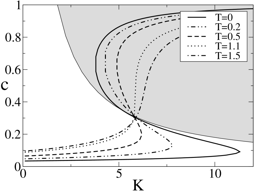
Figure 8: The order parameter $c$ versus coupling strength $K$ for selected values of temperature $T$. The increase of $T$ decreases the region of hysteresis. Remaining parameters are $\tau=2.0$ and $a=2.8$.

IV Summary

In this paper we have investigated the equilibrium and nonequilibrium system of coupled phase oscillators. In fact, it can be any abstract model of interacting particles in spatially periodic structure with a periodic global interaction (e.g. interacting Brownian motors rei2 ; wio ). The equilibrium system defined by eq. (II) is a special case of models considered in the literature. Nevertheless, to the best of our knowledge, the state equation (20) has not been presented. We pay attention to the subtle stability problem which sometimes is treated superficially wio . Properties of the nonequilibrium system (III) are naturally much more interesting. The phase diagram consists of five parts and cannot be fully obtained from the mean-field approach. The non-mean-field regime is the oscillating regime, which has been detected by use of the Monte-Carlo simulations and by analyzing fluctuations of the order parameter $c=\langle\cos x\rangle$. The next interesting finding is that although the non-interacting system is in the diffusive regime, the interaction can move the system to the non-diffusive regime and then “particles” are confined in valleys of the potential (of course it is exact when temperature $T=0$). It means that effectively, for the one-particle dynamics, the barrier height $2\left(1+Kc\right)$ of the local potential is magnified and nonequilibrium fluctuations of amplitude $a$ are not able to induce transitions over barrier.

All the results so far refer to the simple reflection-symmetric local potential $-\cos x$. If we add the higher order harmonics, e.g. $\cos 2x$, the potential is still symmetric. However, behavior of the system can then be radically different because the second order parameter $s=\langle\sin x\rangle\neq 0$. New phenomena such as the symmetry breaking, phase transitions and noise-induced transport can occur in the system. The paper on this subject will be published elsewhere.

References

- [1] S. Shinomoto and Y. Kuramoto, Prog. Theor. Phys. 75, 1105 (1986); H. Sakaguchi, S. Shinomoto and Y. Kuramoto, Prog. Theor. Phys. 79, 600 (1988).
- [2] K. Wiesenfeld and P. Hadley, Phys. Rev. Lett. 62, 1335 (1989); S. Kim and M. Y. Choi, Phys. Rev. B 48, 322 (1993).
- [3] S. H. Strogatz, C. M. Marcus, R. M. Westervelt, and R. E. Mirollo, Physica D 36, 23 (1989).
- [4] Y. Kuramoto, Chemical Oscillations, Waves and Turbulence (Springer, New York, 1984).
- [5] A. Arenas and C. Vicente, Phys. Rev. E 50, 949 (1994).
- [6] A. Winfree, The Geometry of Biological Time (Springer, New York, 1980).
- [7] J. D. Murray, Mathematical Biology (Springer, Berlin, 1993).
- [8] P. Reimann, C. Van den Broeck, and R. Kawai, Phys. Rev. E 60, 6402 (1999).
- [9] S. H. Park and S. Kim, Phys. Rev. E bf 53, 3425 (1996).
- [10] J. Kula, M. Kostur and J. Łuczka, Chem. Phys. 235, 27 (1998).
- [11] C. Van den Broeck and P. Hänggi, Phys. Rev. A 30, 2730 (1984).
- [12] J. Łuczka, Physica A 247, 200 (1999).
- [13] http://mk.phys.us.edu.pl/marcin/coupled
- [14] R. Häussler, R. Bartussek and P. Hänggi, Coupled Brownian Rectifiers, in: Applied Nonlinear Dynamics and Stochastic Systems near the Millennium, AIP Conf. Proc. Vol.411: J. B. Kadtke and A. Bulsara, eds., (American Institute of Physics, New York, 1997) p. 243 - 248; P. Reimann,R. Kawai, C. Van den Broeck, and P. Hänggi, Europhys. Lett. 45, 545 (1999); P. Reimann, Brownian Motors: Noisy Transport far from Equilibrium, Phys. Rep. (in press);
- [15] J. Buceta, J. M. Parrondo, C. Van den Broeck, and F. J. de la Rubia, Phys. Rev. E 61, 6287 (2000); S. E. Mangioni, R. R. Deza, and H. S. Wio ibid. 63 041115 (2001).