Scaling Solutions of Inelastic Boltzmann Equations
with Over-populated High Energy Tails

Abstract

This paper deals with solutions of the nonlinear Boltzmann equation for spatially uniform freely cooling inelastic Maxwell models for large times and for large velocities, and the nonuniform convergence to these limits. We demonstrate how the velocity distribution approaches in the scaling limit to a similarity solution with a power law tail for general classes of initial conditions and derive a transcendental equation from which the exponents in the tails can be calculated. Moreover on the basis of the available analytic and numerical results for inelastic hard spheres and inelastic Maxwell models we formulate a conjecture on the approach of the velocity distribution function to a scaling form.

Pacs: 05.20.Dd (Kinetic theory), 05.20.-y (Classical Statistical Mechanics), 45.70.M (Granular Systems)

Keywords: similarity solutions, power law tails, granular Maxwell model, characteristic functions.

I Introduction

In recent times overpopulation of high energy times in velocity distributions of freely cooling or in driven granular fluids has become a focus of attention in laboratory experiments, kinetic theory and computer simulations [1]. In kinetic theory, granular fluids out of equilibrium were originally modeled by inelastic hard spheres (IHS)[2, 3], which is the proto-typical model for dissipative short ranged hard core interactions. In general, similarity solutions are of interest, because they play an important role as asymptotic or limiting solutions of the Boltzmann equation at large times or at large velocities, and they frequently show overpopulated high energy tails when compared to the omni-present Gaussians.

Overpopulated tails were first found theoretically by studying scaling or similarity solutions of the nonlinear Enskog-Boltzmann equation for the IHS fluid, both in freely evolving IHS systems without energy input [4], as well as in driven or fluidized systems [4, 5, 6], and confirmed afterwards by Monte Carlo simulations of the Boltzmann equation [7, 8], and by laboratory experiments[1]. Overpopulated tails in free IHS fluids [9] and driven ones[10] have also been studied by molecular dynamics simulations of inelastic hard spheres. The observed overpopulations in IHS systems are mainly stretched exponentials $\exp[-Ac^{b}]$ with $b=1$ [11, 4, 7, 8] in systems without energy input, and $b=3/2$[4, 8] in driven systems, but for some forms of driving[8, 5] $b=2$ has been observed. For hard sphere systems there is in general good agreement between the analytic predictions and numerical or Monte Carlo solutions of the nonlinear Boltzmann equation.

About two years ago Boltzmann equations for inelastic Maxwell models have been introduced for the free case without energy input in Ref. [12, 13], and for the driven case in Ref. [14, 15, 16]. In these studies similarity solutions have received a great deal of attention, because general classes of such solutions turned out to be non-positive, and hence unphysical.

The interest in overpopulated tails in elastic Maxwell models has already a long history, and originated from the discovery of an exact positive similarity solution of the nonlinear Boltzmann equation for Maxwell molecules, the so-call BKW mode [17, 18, 19, 20], named after Bobylev, Krook and Wu. The most recent interest in similarity solutions of the Boltzmann equation for inelastic Maxwell models (IMM) was also stimulated by the discovery of an exact similarity solution [21] for a freely cooling one-dimensional IMM of the form $\tilde{f}(c)=(2/\pi)1/[1+c^{2}]^{2}$. It is positive, has finite mean energy $\langle c^{2}\rangle$, and an algebraic high energy tail $1/c^{4}$. The same authors also obtained [21, 22] Monte Carlo solutions $f(v,t)$ of the nonlinear Boltzmann equation for freely evolving IMM systems with general initial distributions both in one and two dimensions, and observed that their numerical results for $f(v,t)$ at large time could be collapsed on a scaling form $f(v,t)\sim(v_{o}(t))^{-d}\tilde{f}(v/v_{o}(t))$. Here $v^{2}_{o}(t)\sim\langle v^{2}\rangle\sim\exp[-\gamma t]$, where the decay rate $\gamma\sim(1-\alpha^{2})$, represents the typical decay of the average kinetic energy. Moreover, these scaling solutions showed heavily overpopulated power law tails with a cross-over time, $\tau_{{\rm tail}}(v)$, that increases with the energy, and $\alpha$ is the coefficient of normal restitution.

Soon after that Krapivsky and Ben-Naim [23] and the present authors [24], using a self-consistent method, gave a theoretical explanation of these power law tails for general dimensionality $d$ together with explicit predictions of the tail exponent $a$, defined through $\tilde{f}(c)\sim 1/c^{2a+d}$. These results were recently extended [25, 26] to driven inelastic Maxwell models, where the high energy tail is of exponential form $~{}\exp[-A|c|]$. Apparently, the type of overpopulation depends sensitively on the microscopic model, on the degree of inelasticity and on the possible mode of energy supply to the dissipative system.

From the point of view of kinetic theory the intriguing question is, what is the generic feature causing overpopulation of high energy tails in systems with inelastic particles, rather than what is the specific shape of the tail. How does the overpopulation depend on the underlying microscopic model, and on the different forms of energy input [8, 5, 14, 15, 16]? As discussed more extensively in Ref. [25] the differences in shape are frequently related to non-uniformities in the limits of long times, large velocities and vanishing inelasticity, which lead to different results when taking the limits in different order or when taking coupled limits such as the scaling limit (e.g. the differences between bulk and tail behavior), or performing an expansion in powers of the inelasticity, and then studying large times (typically Gaussian tails are observed[14]) or studying large times at fixed inelasticity and taking large time limits afterwards (typically overpopulated tails are observed [5, 6]) with a whole wealth of coupled limits in between.

What are inelastic Maxwell models? The IMM’s, introduced in [12, 13], share with elastic Maxwell molecules the property that the collision rate in the Boltzmann equation is independent of the relative kinetic energy of the colliding pair. However, these IMM’s do not describe real particles, but only pseudo-particles with ’collision rules’ $({\bf v}_{1},{\bf v}_{2})\to({\bf v}^{*}_{1},{\bf v}^{*}_{2})$ between pre- and post-collision velocities, defined to be the same as for smooth inelastic hard spheres with a restitution coefficient $\alpha$ with $(0<\alpha<1)$. There are no such objects as ’inelastic Maxwell particles’ that interact according to a given force law and that can be studied by molecular dynamics simulations.

These IMM’s are of interest for granular fluids in spatially homogeneous states, not because they can claim to be more realistic than IHS’s, but because of the mathematical simplifications resulting from an energy-independent collision rate. Nevertheless the IMM’s keep the qualitatively correct structure and properties of the nonlinear macroscopic equations [27] and obey Haff’s law [28], just like the even simpler inelastic BGK or single relaxation time models [29] do. What harmonic oscillators are for quantum mechanics, and dumb-bells for polymer physics, that is what elastic and inelastic Maxwell models are for kinetic theory.

From the point of view of nonequilibrium (steady) states, the structure of velocity distributions in dissipative systems, including the high energy tail, is a subject of continuing research, as the universality of the Gibbs’ state of thermal equilibrium is lacking outside thermal equilibrium, and a possible classification of generic structures would be of great interest in many fields of non-equilibrium statistical mechanics.

After this explanation of the possible relevance of inelastic Maxwell models for different fields of research, we concentrate on the kinetic theory for these models, in particular on the simplest case, the freely cooling one without energy input. We return now to the recent results of Refs.[21, 30, 22], and we consider their observations, described above, as strong evidence for the existence of interesting limiting behavior when coupled limits are taken, and more explicitly, we interpret their findings as follows: the transformed or rescaled distribution function $\tilde{f}(c,t)$ defined through,

$$f(v,t)=(v_{o}(t))^{-d}\tilde{f}(v/v_{o}(t),t),$$ (I.1)

approaches a scaling or similarity form in the coupled limit as $t\to\infty$ and $v\to 0$, with $v/v_{o}(t)=c$ kept constant, i.e.

$$\lim_{t\to\infty}\tilde{f}(c,t)=\lim_{t\to\infty}(v_{o}(t))^{d}f(v_{o}(t)c,t)=\tilde{f}(c).$$ (I.2)

The coupled limit considered in (I.2) is the same scaling limit as considered in the solutions of the nonlinear Boltzmann equation for IHS in Refs.[4, 25], although it has not been pointed out so emphatically. On the other hand the scaling limit, considered in Refs. [13, 14, 15, 16], is the coupled limit as $t\to\infty$ and $\alpha\to 1$ with $(1-\alpha^{2})t=const$, while $v$ is kept constant.

The present paper leads to the formulation of a conjecture by combining the recent results on scaling solutions and overpopulated high energy tails in inelastic hard sphere fluids and inelastic Maxwell models with an older conjecture of Krook and Wu [19] on the role of a special self-similar solution, the so-called BKW-mode [17, 18, 19, 20], named after Bobylev, Krook and Wu. This conjecture reads: Solutions $f(v,t)$ of the nonlinear Boltzmann equation for dissipative systems – i.e. the rescaled distribution $\tilde{f}(c,t)$ in (I.1) rescaled with the instantaneous r.m.s. velocity $v_{o}(t)\sim(\langle v^{2}\rangle)^{1/2}$ – approach for general initial conditions, in the scaling limit (I.2), to the scaling solution $\tilde{f}(c)$ with an overpopulated high energy tail. In taking the scaling limit the degree of inelasticity, $(1-\alpha^{2})$, must be kept constant, and cannot be interchanged with the elastic limit $({\alpha}\uparrow 1)$.

This conjecture is a variation on the Krook-Wu conjecture for elastic Maxwell molecules, formulated as: ”An arbitrary initial state tends first to relax to a state, characterized by the BKW-mode. The subsequent relaxation is essentially represented the BKW-mode with an appropriate phase”. As it turned out, this conjecture was not supported by numerical and analytic results obtained for the physically most relevant initial distributions with a finite second moment in the limit as $t\to+\infty$[20]. However, Bobylev and Cercignani have recently shown that the conjecture holds in systems of elastic Maxwell molecules in the limit $t\to-\infty$ for the so-called eternal solutions $f(v,t)$[31, 32], which are characterized by a divergent second moment.

The paper is organized as follows. In section II the mathematical model Boltzmann equation for IMM’s is constructed starting from the Enskog-Boltzmann equation for IHS’s, and some basic properties are derived there, as well as in Appendix A. In section III we show that the IMM Boltzmann equation admits a similarity solution with a power law tail $\sim 1/c^{2a+d}$, where the non-integer tail exponent $a$ is the solution of a transcendental equation, which is solved numerically. The moments $\langle c^{2n}\rangle$ of the scaling form $\tilde{f}{(c)}$ with $n<a$ are calculated in section IV.B from a recursion relation. The moments with $n>a$ are divergent. In section IV.B we demonstrate that the moment $\mu_{n}(t)$ of the rescaled distribution $\tilde{f}(c,t)$, for the general class of initial conditions with all moments $\langle v^{2n}\rangle<\infty$, approach in the long time limit for $n<a$ to the unique set of moments $\mu_{n}$ of the scaling form, and we analyze how all moments $\mu_{n}(t)\to\infty$ for $n>a$. Some generalizations of these results are described in section IV.C. In section V we present our conclusions, and interpret our results as a demonstration of our conjecture for IMM’s, i.e. as a weak form of approach of an arbitrary rescaled distribution $\tilde{f}(c,t)$ to a universal scaling form.

II Kinetic Equations for Dissipative Systems

A Inelastic Hard Spheres

For the construction of inelastic Maxwell models, it is convenient to start from the spatially homogeneous Boltzmann equation for inelastic hard spheres. We study the velocity distribution, $f({\bf v},\tau)$ in the so-called homogeneous cooling state (HCS). Here $\tau$ is the ”external” laboratory time, and the relation to time $t$ used in section I will be given in due time. Moreover we restrict ourselves to isotropic distributions $f(v,\tau)$ with $v=|{\bf v}|$ with isotropic initial conditions, $f(v,0)$. The most basic and most frequently used model for dissipative systems with short range hard core repulsion is the Enskog-Boltzmann equation for inelastic hard spheres in $d-$dimensions [2],

$${\partial}_{\tau}f_{1}=I(f)\equiv 2\int_{\bf n}\int d{\bf v}_{2}\theta({{\bf v}}_{12}\cdot{\bf n})|{{\bf v}}_{12}\cdot{\bf n}|[\textstyle{\frac{1}{{\alpha}^{2}}}f_{1}^{**}f_{2}^{**}-f_{1}f_{2}],$$ (II.1)

where $f_{1}^{**}$ is short for $f({\bf v}_{1}^{**},\tau)$, and we have absorbed constant factors in the time scale. Velocities and time have been dimensionalized in terms of the width and the mean free time of the initial distribution, and $|{{\bf v}}_{12}\cdot{\bf n}|$ is essentially the dimensionless collision rate. Moreover, $\int_{\bf n}(\cdots)=(1/\Omega_{d})\int d{\bf n}(\cdots)$ is an angular average over a $d$-dimensional unit sphere, restricted to the hemisphere, ${{\bf v}}_{12}\cdot{\bf n}>0$, through the unit step function $\theta(x)$, and $\Omega_{d}=2\pi^{d/2}/\Gamma(\textstyle{\frac{1}{2}}d)$.

The velocities ${{\bf v}}_{i}^{**}$ with $i,j=\{1,2\}$ denote the restituting velocities, and ${\bf v}_{i}^{*}$ the corresponding direct postcollision velocities. They are defined as,

$${\bf v}_{i}^{**} = {\bf v}_{i}-\textstyle{\frac{1}{2}}(1+\textstyle{\frac{1}{{\alpha}}}){\bf v}_{ij}\cdot{\bf n}{\bf n}$$ (II.2)

$${\bf v}_{i}^{*} = {\bf v}_{i}-\textstyle{\frac{1}{2}}(1+{\alpha}){\bf v}_{ij}\cdot{\bf n}{\bf n}.$$ (II.3)

Here ${\alpha}$ is the coefficient of restitution $(0<{\alpha}<1)$, the relative velocity is ${\bf v}_{ij}={\bf v}_{i}-{\bf v}_{j}$, and ${\bf n}$ is a unit vector along the line of centers of the interacting particles. In one dimension the angular average $\int_{\bf n}$, as well as the dyadic product ${\bf n}{\bf n}$ can be replaced by the number $1$. One of the factors $(1/{\alpha})$ in Eq.(II.1) originates from the Jacobian, $d{\bf v}_{1}^{**}d{\bf v}_{2}^{**}=(1/{\alpha})d{\bf v}_{1}d{\bf v}_{2}$, and the other one from the collision rate of the restituting collisions, $|{{\bf v}}^{**}_{12}\cdot{\bf n}|=(1/{\alpha})|{{\bf v}}_{12}\cdot{\bf n}|$. Furthermore, in the HCS symmetrization over ${\bf n}$ and $-{\bf n}$ allows us to replace $2\theta(x)$ in (II.1) by $1$.

In subsequent sections we will also need the rate equations for the average $\langle\psi\rangle_{\tau}=\int d{\bf v}\psi({\bf v})f({\bf v},\tau)$, as follows from the Boltzmann equation,

$$d\langle\psi\rangle_{\tau}/d\tau=\textstyle\int d{\bf v}\psi({\bf v})I(f)=\int_{\bf n}\int d{\bf v}_{1}d{\bf v}_{2}|{{\bf v}}_{12}\cdot{\bf n}|f_{1}f_{2}[\psi({\bf v}^{*}_{1})-\psi({\bf v}_{1})].$$ (II.4)

The Boltzmann collision operator conserves the number of particles $(\psi({\bf v})=1)$ and momentum $(\psi({\bf v})={\bf v})$, but not the energy $(\psi({\bf v})=v^{2})$. Here normalizations are chosen such that,

$$\langle 1\rangle_{\tau} =\int d{\bf v}f({\bf v},\tau) =1$$ (II.5)

$$\langle{\bf v}\rangle_{\tau} =\int d{\bf v}{\bf v}f({\bf v},\tau) =0$$ (II.6)

$$\langle v^{2}\rangle_{\tau} =\int d{\bf v}v^{2}f({\bf v},\tau) =\textstyle{\frac{1}{2}}dv_{o}^{2}(\tau).$$ (II.7)

As a consequence of the inelasticity an amount of energy, $\textstyle{\frac{1}{4}}(1-{\alpha}^{2})[{{\bf v}}_{12}\cdot{\bf n}]^{2}$, is lost in every inelastic collision. Consequently the average kinetic energy or granular temperature $\langle v^{2}\rangle$ keeps decreasing at a rate proportional to the inelasticity $(1-{\alpha}^{2})$. So, the solution of the Boltzmann equation does not reach thermal equilibrium, described by the Maxwellian $\varphi_{o}({\bf v})=\pi^{-d/2}\exp[-v^{2}]$, but is approaching a Dirac delta function $\delta^{(d)}({\bf v})$ for large times. As the convergence of $f(v,\tau)$ to its limiting value as $\tau\to\infty$ is in general non-uniform, the rescaled distribution may approach a different limit (see (I.2)). Also, the detailed balance condition is violated, and the Boltzmann equation does not obey an $H-$theorem. The moment equations and the behavior of the scaling solutions for freely evolving and driven IHS fluids have been extensively discussed both in the bulk of the thermal distribution, as well as in the high energy tails [7, 4].

B Inelastic Maxwell Models

One of the difficulties in solving the nonlinear Boltzmann equation (II.1) for hard spheres is that the collision rate $|{\bf v}_{12}\cdot{\bf n}|$ is not a constant, but is proportional to the relative velocity $v_{12}$ of the colliding pair, which is typically of order $v_{12}\sim v_{o}(\tau)$, as defined in (II.5). Maxwell models on the other hand are defined to have a collision rate independent of the relative energy of the colliding particles.

In the recent literature two different types of mathematical simplifications have been introduced which convert the IHS- Boltzmann equation into one for an inelastic Maxwell model with an energy independent collision rate. In the most drastic simplification, the IMM-A discussed in Refs. [30, 23, 24], one replaces the collision rate $|{\bf v}_{12}\cdot{\bf n}|$ for the direct collisions, as well as the one for the restituting collisions, $|{\bf v}^{**}_{12}\cdot{\bf n}|=|{\bf v}_{12}\cdot{\bf n}|/{\alpha}$ by its typical mean value $v_{o}(\tau)$. In a more refined approximation Bobylev et al. [13] replace these collision rates by $v_{o}(\tau)|\hat{{\bf v}}_{12}\cdot{\bf n}|$. We call this model IMM-B. Both approximations keep the qualitatively correct dependence of the total energy $v_{o}^{2}(\tau)$ on the ’external’ time $\tau$. In fact, strictly speaking these models should be called pseudo-Maxwell molecules, because there do not exist microscopic particles with dissipative interparticle forces, for which the mathematical model Boltzmann equations below can be derived.

By making the above mathematical simplifications we obtain from (II.1) a collision term which is multiplied by a factor $v_{o}(\tau)$. This factor is then absorbed by introducing a new time variable $t$. For model IMM-A the resulting time transformation and Boltzmann equation in dimensionless variables are then given by,

$$dt = v_{o}(\tau)d\tau$$ (II.8)

$$\partial_{t}f_{1} = I(f)=\int_{\bf n}\int d{\bf v}_{2}\left[\textstyle{\frac{1}{{\alpha}}}f_{1}^{**}f_{2}^{**}-f_{1}f_{2}\right]$$ (II.9)

$$= -f_{1}+\int_{\bf n}\int d{\bf v}_{2}\textstyle{\frac{1}{{\alpha}}}f_{1}^{**}f_{2}^{**}.$$ (II.10)

For the IMM-B we introduce a slightly different time variable $t$, and obtain the Boltzmann equation in dimensionless variables,

$$dt = \beta_{1}v_{o}(\tau)d\tau$$ (II.11)

$$\partial_{t}f_{1} = I(f)=\int^{\prime}_{\bf n}\int d{\bf v}_{2}|\hat{{\bf v}}_{12}\cdot{\bf n}|\left[\textstyle{\frac{1}{{\alpha}}}f_{1}^{**}f_{2}^{**}-f_{1}f_{2}\right]$$ (II.12)

$$= -f_{1}+\int^{\prime}_{\bf n}\int d{\bf v}_{2}|\hat{{\bf v}}_{12}\cdot{\bf n}|\textstyle{\frac{1}{{\alpha}}}f_{1}^{**}f_{2}^{**},$$ (II.13)

where $\int^{\prime}_{\bf n}=(1/\beta_{1})\int_{\bf n}$ with $\beta_{1}$ defined in (A.1). The prefactors in the time transformations are chosen such that the loss term takes the simple form $-f_{1}$. This implies that the new time variable $t(\tau)$ counts the average number of collisions suffered by a particle within the ”external” time $\tau$. Hence $t$ is the collision counter or ”internal” time of a particle.

One of the important properties of Maxwell models is that the moment equations form a set of coupled equations, that can be solved sequentially. For the one-dimensional Maxwell model these equations were derived in Ref.[12], and for the three-dimensional model IMM-B with uniform impact parameter this was done in Ref.[13]. The general moment equations for the present Maxwell models will be derived after having obtained the characteristic function in Sect.III. At this point we make an exception for the second moment, which determines the typical velocity $v_{o}(t)$ through the relation $\langle v^{2}\rangle_{t}=\textstyle{\frac{1}{2}}dv_{o}^{2}(t)$, needed to study the rescaled distribution function. It follows from the kinetic equations (II.8) and (II.11) as

$$\partial_{t}\langle v^{2}\rangle_{t} =-\gamma\langle v^{2}\rangle_{t}$$ (II.14)

$$\gamma =\left\{\begin{array}[]{ll}\frac{1-{\alpha}^{2}}{2d}=\frac{2p(1-p)}{d}&\qquad\mbox{(IMM-A)}\\[2.84526pt] \frac{1-{\alpha}^{2}}{d+1}=\frac{4p(1-p)}{d+1}&\qquad\mbox{(IMM-B)}\end{array}\right.,$$ (II.17)

where $p=\textstyle{\frac{1}{2}}(1+{\alpha})$. Consequently $v_{o}(t)=v_{o}(0)\exp[-\textstyle{\frac{1}{2}}\gamma t]$. Moreover, by solving the differential equations for $t$ in (II.8) and (II.11) we obtain the relations between the internal time $t$ and the external time $\tau$, i.e.

$$\exp[\textstyle{\frac{1}{2}}\gamma t]=\left\{\begin{array}[]{ll}1+\textstyle{\frac{1}{2}}\gamma v_{o}(0)\tau&\qquad\mbox{(IMM-A)}\\[2.84526pt] 1+\textstyle{\frac{1}{2}}\beta_{1}\gamma v_{o}(0)\tau&\qquad\mbox{(IMM-B)}\end{array}\right.,$$ (II.18)

as well as the decay of the energy in terms of internal time $t$ and external time $\tau$, i.e.

$$v^{2}_{o}(t)=\exp[-\gamma t]v^{2}_{o}(0)=\left\{\begin{array}[]{ll}v^{2}_{o}(0)/[1+\textstyle{\frac{1}{2}}\gamma v_{o}(0)\tau]^{2}&\qquad\mbox{(IMM-A)}\\[2.84526pt] v^{2}_{o}(0)/[1+\textstyle{\frac{1}{2}}\beta_{1}\gamma v_{o}(0)\tau]^{2}&\qquad\mbox{(IMM-B)}.\end{array}\right..$$ (II.19)

This shows that Haff’s law [28], given by the second equality, is also valid for inelastic Maxwell models.

To further elucidate the difference between the two classes of models we change the integration variables ${\bf n}$ — which specifies the point of incidence on a $d$-dimensional action sphere of two colliding particles — to the impact parameter, $b=|\hat{{\bf v}}_{12}\times{\bf n}|=\sin\theta$, where $\theta=\cos^{-1}(\hat{{\bf v}}_{12}\cdot{\bf n})$ is the angle of incidence. The relevant structure of the integrals for IMM-A and IMM-B is respectively,

$$\int_{\bf n} \sim\displaystyle\int^{\pi/2}_{0}d\theta(\sin\theta)^{d-2}\sim\int^{1}_{0}dbb^{d-2}/\sqrt{1-b^{2}}$$ (II.20)

$$\int^{\prime}_{{\bf n}}|\hat{{\bf v}}_{12}\cdot{\bf n}| \displaystyle\sim\int^{\pi/2}_{0}d\theta(\sin\theta)^{d-2}\cos\theta\sim\int^{1}_{0}dbb^{d-2}$$ . (II.21)

Therefore model A has a uniform distribution ${\cal P}(\theta)=1$ over angles of incidence, and a non-uniform distribution $P(b)=1/\sqrt{1-b^{2}}$ over impact parameters, which is biased towards grazing collisions, where $b=1$. Model B has a uniform distribution $P(b)=1$ over impact parameters, and a non-uniform distribution, ${\cal P}(\theta)=\cos\theta$, biased towards zero angle of incidence. In this context it is important to note that the arguments on the validity of the Boltzmann equation are based on the assumption of molecular chaos, i.e. absence of precollision correlations between the velocities of a colliding pair. This implies that the distribution function of impact parameters be uniform. Hence, model IMM-A does not obey molecular chaos.

The question of interest in then: do IMM-A and IMM-B yield qualitatively the same results for the scaling distribution? The question is relevant because Molecular Dynamics simulations (MD) of a system of $N$ IHS have shown that the dissipative dynamics (II.2) drives an initially uniform distribution $P(b)=1$ in the HCS towards a non-uniform distribution $P(b)$, biased towards grazing collisions, which violates molecular chaos. So the IMM-A model with a built-in initial bias may lead to spurious effects, such as power law tails in $f(v,t)$, which are artifacts of a too drastic simplification.

C Similarity Solutions

The questions addressed in this subsection are: do the Boltzmann equations for the Maxwell models, constructed in the previous section, admit similarity solutions, and what are the properties of such solutions? We define a similarity solution $\tilde{f}(c)$ through the relation,

$$f({\bf v},t)=v_{o}^{-d}(t)\tilde{f}({\bf v}/v_{o}(t)).$$ (II.22)

The normalizations imposed by (II.5) on these solutions are,

$$\int d{\bf c}\tilde{f}({\bf c})=1\qquad\int d{\bf c}\;c^{2}\tilde{f}({\bf c})=\textstyle{\frac{1}{2}}d.$$ (II.23)

By inserting (II.22) in (II.1), and using $v_{o}(t)\sim\exp[-\textstyle{\frac{1}{2}}\gamma t]$ we obtain the following integral equation for $\tilde{f}(c)$, i.e.

$$\textstyle{\frac{1}{2}}{\gamma}\frac{{\bf\partial}}{{\bf\partial}{\bf c}}\cdot{\bf c}\tilde{f}(c)=\widetilde{I}(\tilde{f}).$$ (II.24)

Here the operator $\tilde{I}(\tilde{f})$ has the same functional form as $I(f)$ in (II.8) or (II.11) with $\{{\bf v}_{i},f\}$ replaced by $\{{\bf c}_{i},\tilde{f}\}$.

One of the goals of this paper is also to analyze in section IV in what sense the rescaled distribution function, $\tilde{f}(c,t)$, approaches its limiting form as $t\to\infty$. To do so, we also need the kinetic equation for the rescaled $\tilde{f}(c,t)$, which reads,

$$\partial_{t}\tilde{f}+\textstyle{\frac{1}{2}}{\gamma}\frac{{\bf\partial}}{{\bf\partial}{\bf c}}\cdot{\bf c}\tilde{f}=\tilde{I}(\tilde{f}).$$ (II.25)

Some comments are in order here. Physical solutions $\tilde{f}({\bf c})$ of (II.24) must be non-negative. A velocity distribution $f({\bf v},t)$, evolving under the nonlinear Boltzmann equation, preserves positivity for a positive initial distribution $f({\bf v},0)$ [33, 34]. However, for scaling solutions, being the solution of (II.24), positivity is not guaranteed [13, 20]. If one would know a positive scaling solution $\tilde{f}(c)$ – as is the case in one dimension [21] – and prepare the system in this initial state, then the entropy $S$ or the $H-$function in state (II.22), also shows singular behavior, i.e.

$$S(t) = -H(t)=-\int d{\bf c}\tilde{f}({\bf c})\ln{\tilde{f}({\bf c})}-\textstyle{\frac{1}{2}}d\gamma t+const$$ (II.26)

$$\simeq -\textstyle{\frac{1}{2}}d\,\gamma\,t+const\qquad(t\;\;{\rm large}),$$ (II.27)

where $\gamma$ is positive and $\int\tilde{f}\ln\tilde{f}$ is some constant. In these solutions the entropy keeps decreasing at a constant rate $\textstyle{\frac{1}{2}}d\;\gamma$. This is typical for pattern forming mechanisms in configuration space, where spatial order or correlations are building up, as well as in dynamical systems and chaos theory, where the rate of irreversible entropy production is negative on an attractor [35, 36, 37]. In fact the forward dissipative dynamics, $({\bf v}_{1},{\bf v}_{2})\to({\bf v}_{1}^{*},{\bf v}_{2}^{*})$, defined in (II.2), has a Jacobian $J={\alpha}<1$, i.e. $d{\bf v}_{1}^{*}d{\bf v}_{2}^{*}={\alpha}d{\bf v}_{1}d{\bf v}_{2}$, corresponding to a contracting flow in ${\bf v}-$space. Moreover, there is no fundamental objection against decreasing entropies in an open subsystem, here the inelastic Maxwell particles, interacting with a reservoir. The reservoir is here the sink, formed by the dissipative collisions, causing the probability to contract onto an attractor.

III Power Law Tails

A Fourier transformed Boltzmann equation

The goal of this section is to show that the Boltzmann equation for IMM’s has a scaling solution with a power law tail. This is done by introducing the Fourier transform of the distribution function, $\varphi({\bf k},t)=\langle\exp[-i{\bf k}\cdot{{\bf v}}]\rangle_{t}$, which is the characteristic function or generating function of the velocity moments. Because $f(v,t)$ is isotropic, $\varphi(k,t)$ is isotropic as well. It is also convenient to consider $\phi(x,t)$, defined through the relation $\varphi(k,t)=\phi(\textstyle{\frac{1}{4}}k^{2},t)$.

We start with the simplest case, and apply Bobylev’s Fourier transform method [13, 18] to the Boltzmann equation (II.8) for model IMM-A with the result,

$$\partial_{t}\varphi({\bf k},t) = \int_{\bf n}[\varphi({\bf k}_{+},t)\varphi({\bf k}_{-},t)-\varphi({\bf 0},t)\varphi({\bf k},t)]$$ (III.1)

$$\partial_{t}\phi(x,t) = \int_{\bf n}[\phi(xe_{+}({\bf n}),t)\phi(xe_{-}({\bf n}),t)-\phi(0,t)\phi(x,t)],$$ (III.2)

where $\varphi({\bf 0},t)=1=\phi(0,t)$. Here we have used (II.4) with $\psi({\bf v}_{1})=\exp[-i{\bf k}\cdot{\bf v}^{*}_{1}]$ and expressed the exponent as ${\bf k}\cdot{\bf v}^{*}_{1}={\bf k}_{-}\cdot{\bf v}_{1}+{\bf k}_{+}\cdot{\bf v}_{2}$ (see (II.2)), where

$${\bf k}_{+} \equiv k\tilde{{\bf k}}_{+}=p{\bf k}\cdot{\bf n}{\bf n}\qquad \tilde{k}_{+}^{2}=p^{2}(\hat{{\bf k}}\cdot{\bf n})^{2}=e_{+}({\bf n})$$ (III.3)

$${\bf k}_{-} \equiv k\tilde{{\bf k}}_{-}={\bf k}-{\bf k}_{+}\qquad \tilde{k}_{-}^{2}=[1-z(\hat{{\bf k}}\cdot{\bf n})^{2}]=e_{-}({\bf n}),$$ (III.4)

with $p=\textstyle{\frac{1}{2}}(1+{\alpha})$ and $z=2p-p^{2}$. In one dimension this equation simplifies to

$$\partial_{t}\varphi(k,t)=\varphi(pk,t)\varphi((1-p)k,t)-\varphi(k,t),$$ (III.5)

where $k_{+}=pk$ and $k_{-}=(1-p)k$. Equation (III.1) has the interesting property that for a given solution $\varphi({\bf k},t)$ one has a whole class of solutions $\overline{\varphi}({\bf k},t)=\exp[i{\bf k}\cdot{\bf w}]\varphi({\bf k},t)$ where ${\bf w}$ is an arbitrary velocity vector [18, 13]. This property reflects the Galilean invariance of the Boltzmann equation.

Because $f(v,t)$ is isotropic, only its even moments are non-vanishing, and the moment expansion of the characteristic function then takes the form,

$$\varphi({\bf k},t)=\sum_{m=even}\frac{(-ik)^{m}}{m!}\langle(\hat{\bf k}\cdot{\bf v})^{m}\rangle_{t}=\sum_{n}\frac{(-x)^{n}}{n!}m_{n}(t)=\phi(x,t),$$ (III.6)

where $x=k^{2}/4$. The angular time independent average $\langle(\hat{\bf k}\cdot\hat{\bf v})^{2n}\rangle=\beta_{2n}$ is calculated in (A.1) and the moment $m_{n}(t)$ is defined as

$$m_{n}(t)=4^{n}n!\beta_{2n}\langle v^{2n}\rangle_{t}/(2n)!=\langle v^{2n}\rangle_{t}/(d/2)_{n}$$ (III.7)

$$\beta_{2n}=\langle(\hat{\bf k}\cdot\hat{\bf v})^{2n}\rangle=(1/2)_{n}/(d/2)_{n}$$ . (III.8)

The Pochhammer symbol $(a)_{n}$ is defined in (A.3) and we have used the duplication formula for the Gamma function $(2n)!=\Gamma(2n+1)$. Furthermore we note that the moments of a Gaussian $\varphi_{o}(v)=\pi^{-d/2}\exp(-v^{2})$ are $\langle v^{2n}\rangle_{o}=(d/2)_{n}$.

Scaling solutions in Fourier representation have the form $\phi(x,t)=\Phi(e_{o}(t)x)$, where $\Phi(\textstyle{\frac{1}{4}}k^{2})$ is the Fourier transform of $\tilde{f}(c)$ and $e_{o}(t)=v_{o}^{2}(t)=e^{-\gamma t}e_{o}(0)$. Substitution in Eq.(III.1) yields the integral equation for the scaling form,

$$-\gamma x\Phi^{\prime}(x)+\Phi(x)=\int_{\bf n}\Phi(xe_{+})\Phi(xe_{-}).$$ (III.9)

Its moments follow from the expansion,

$$\Phi(x)=\sum_{n}(-x)^{n}\mu_{n}/n!=1-x+x^{2}\mu_{2}/2!+\cdots$$ (III.10)

$$\mu_{n}=\int d{\bf c}c^{2n}\tilde{f}(c)/(d/2)_{n}\equiv\langle c^{2n}\rangle/(d/2)_{n},$$ (III.11)

where (II.23) imposes $\mu_{1}=1$.

B Small-$k$ singularity of characteristic function

In case all coefficients in the Taylor expansion (III.10) exist, then $\Phi(x)$ is regular at the origin, and the corresponding scaling form $\tilde{f}(c)$ falls off exponentially fast at large $c$, and all its moments $\langle c^{2n}\rangle$ are finite. Suppose now that the small-$k$ or small-$x$ behavior of $\Phi(x)$ contains a singular term $x^{a}$, where $a$ does not take integer values (note that even powers $k^{2a}=k^{2n}$ represent contributions that are regular at small $k$), then its inverse Fourier transform scales as $1/c^{2a+d}$ at large $c$. For this distribution the moments with $n\geq a$ are divergent, and so is the $n$-th derivative of the generating function $\Phi(x)$ at $x=0$. The requirement that the total energy be finite imposes the lower bound $a>1$ on the exponent because of the normalization (II.23).

Model IMM-A

To test whether the Fourier transformed Boltzmann equation (III.1) admits a scaling solution with a dominant small-$x$ singularity $x^{a}$, we make for the small$-x$ ansatz,

$$\Phi(x)=1-x-Ax^{a},$$ (III.12)

insert this expression in (III.9), and investigate whether the resulting equation admits a solution for the exponent $a$. This is done by equating the coefficients of equal powers of $x^{s}$ on both sides of the equation, which yields for general dimensionality,

$$\gamma = \lambda_{1}\equiv\int_{\bf n}[1-e_{+}({\bf n})-e_{-}({\bf n})]=2p(1-p)/d$$ (III.13)

$$a\gamma = \lambda_{a}\equiv\int_{\bf n}[1-e_{+}^{a}({\bf n})-e_{-}^{a}({\bf n})].$$ (III.14)

The eigenvalue $\lambda_{s}(s=1,a)$ has been calculated in (A.6) and (A.23) of the Appendix. The relevant properties are: (i) $\lambda_{0}=0$ because of particle conservation; (ii) $\lim_{s\to 0}\lambda_{s}=-1$; (iii) $\lambda_{s}$ is a concave function, monotonically increasing with $s$, and (iv) all eigenvalues for non-negative integers $n$ are positive (see Fig.1). In one dimension the above eigenvalue becomes $\lambda_{a}=1-p^{2a}-(1-p)^{2a}$.

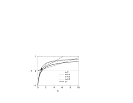
FIG. 1.: Eigenvalue $\lambda_{s}$ is a concave function of $s$, plotted for different values of $\alpha$ for the 2-D inelastic Maxwell model IMM-A. The line $y=s\lambda_{1}$ is plotted for $\alpha=0.6,0.8$ and ${\alpha}=1$(top to bottom). The intersections with $\lambda_{s}$ determine the points $s_{0}$ (filled circles) and $s_{1}$ (open circles). Here $s_{1}=a$ determines the exponent of the power law tail. For the elastic case (${\alpha}=1,\lambda_{1}=0$, energy conservation) there is only 1 intersection point. The branch of $\lambda_{s}$ in the interval $s_{0}<s<s_{1}$ is referred to as stable and the branches $s<s_{0}$ and $s>s_{1}$ as unstable.

To continue we combine both relations in (III.13), which determine the exponent $a$ as the root of the transcendental equation,

$$\lambda_{s}=s\lambda_{1}.$$ (III.15)

This equation has been solved numerically, and the results are plotted in Fig.2. We note here that Krapivsky and Ben-Naim [23] have derived the same transcendental equation.

As can be seen from the graphical solution in Fig.1, the transcendental equation (III.15) has two solutions, the trivial one $(s_{0}=1)$ and the solution $s_{1}=a$ with $a>1$. The numerical solutions for $d=2,3$ are shown in Fig.2a as a function of $\alpha$, and the $\alpha$-dependence of the root $a(\alpha)$ can be understood from the graphical solution in Fig.1. In the elastic limit as $\alpha\uparrow 1$ the eigenvalue $\lambda_{1}(\alpha)\to 0$ because of energy conservation. In that limit the transcendental equation (III.15), $\lambda_{s}(1)-s\lambda_{1}(1)=0$, no longer has a solution with $a>1$, and $a(\alpha)\to\infty$, as it should be. This is consistent with a Maxwellian tail distribution in the elastic case. Needless to say that the transcendental equation for the one-dimensional IMM-A has the solutions $s_{0}=1$ (trivial) and $s_{1}=a=3/2$, describing a power law tail $\tilde{f}(c)\sim 1/|c|^{2a+d}=|c|^{4}$, in full agreement with the exact scaling solution $\tilde{f}(c)=(2/\pi)(1+c^{2})^{-2}$, found by Baldassarri et al. [21] for this case. The one-dimensional case is a bit pathological because the intersection points $(s_{0},s_{1})=(1,3/2)$ of $y=\lambda_{s}(\alpha)$ and $y=s\lambda_{1}(\alpha)$ are independent of $p=\textstyle{\frac{1}{2}}(1+{\alpha})$, implying that these points are common to all $\lambda-$curves at different parameter values ${\alpha}$. In summary, we conclude that there exists for inelastic Maxwell models a scaling solution $\tilde{f}(c)$ with a power law tail $1/|c|^{2a+d}$ at large energies.

As a parenthesis we apply the previous analysis for similarity solutions to the elastic case $(\alpha=1)$, where the BKW - mode, discussed in the introduction, is an exact similarity solution. In the elastic case similarity solutions of (III.1) would also have the form $\phi(x,t)=\Phi(\varepsilon_{o}(t)x)$, but the time dependent factor $\varepsilon_{o}(t)$ is not determined by the conserved second moment $\langle v^{2}\rangle=\textstyle{\frac{1}{2}}d$. So the typical time scale $\gamma$, entering through $\varepsilon_{o}(t)=\exp(-\gamma t)$, will be determined by the lowest moment with $t-$dependence, i.e. $\langle v^{4}\rangle\sim\varepsilon_{o}^{2}(t)$, and its rate equation imposes $\lambda_{2}=2\gamma$. The transcendental equation becomes then $\gamma_{s}=\lambda_{s}-s\lambda_{2}/2$, which has again two solutions, $s_{0}=2$ and $s_{1}=3$ because $\lambda_{2}/2=\lambda_{3}/3$. As both $a$-values are integers, the small$-x$ behavior of the characteristic function contains only regular terms $x^{2}$ and $x^{3}$, which do not result in any power law tails. In fact, the solutions $\{s=2,3\}$ correspond to the exact closed form solution $\phi(x)=e^{-x}(1+x)$, the well-known Bobylev-Krook-Wu mode for elastic Maxwell molecules [18, 20].

FIG. 2.: Exponent $a({\alpha})$, which is the root of (III.15), as a function of the coefficient of restitution $\alpha$, which determines the high energy tail $1/c^{2a+d}$ of the scaling solution $\tilde{f}(c)$. Left panel for IMM-A with uniform angle of incidence in 2-and 3-D, and right panel for IMM-B with uniform impact parameter in 3-D.

Model IMM-B

The second part of this section deals with the Boltzmann equation (II.11) for model IMM-B with uniform impact parameters, as introduced by Bobylev et al. [13], and we show that the above method gives similarity solutions with power law tails for this model as well. We restrict the analysis to the three-dimensional case. The integral equation for the characteristic function in this case has been derived in [13], and reads,

$$\partial_{t}\phi({\bf k},t)=\int^{\prime}_{\bf n}\;|\widehat{{\bf k}}\cdot{\bf n}|\phi({\bf k}_{+},t)\phi({\bf k}_{-},t)-\phi({\bf k},t).$$ (III.16)

In a similar way as in the previous section, we derive the integral equation for the corresponding scaling solution, $\phi(x,t)=\Phi(xe_{o}(t))$ with the result,

$$-\gamma x\Phi^{\prime}(x)+\Phi(x)=\int^{\prime}_{\bf n}|\widehat{{{\bf k}}}\cdot{\bf n}|\Phi(xe_{+})\Phi(xe_{-}),$$ (III.17)

and the procedure described in (III.12) and (III.13) leads to the same transcendental equation (III.15) with eigenvalue,

$$\lambda_{a} = \int^{\prime}_{\bf n}\;|\widehat{{{\bf k}}}\cdot{\bf n}|[1-e_{+}^{a}-e_{-}^{a}]$$ (III.18)

$$= 2\int^{1}_{0}dx\,x\{1-p^{2a}x^{2a}-[1-zx^{2}]^{a}\}$$ (III.19)

$$= 1-\frac{p^{2a}}{a+1}-\frac{1}{a+1}\left\{\frac{1-(1-p)^{2a+2}}{1-(1-p)^{2}}\right\}.$$ (III.20)

The equality on the second line has been obtained by changing to the new integration variable $x=\cos\theta$, and the value for $\lambda_{a}$ is in agreement with the corresponding eigenvalue obtained in [13] for integer $a$. For $a=1$ one obtains here $\lambda_{1}=p(1-p)$, in agreement with (II.14) for d=3. The numerical solution of the transcendental equation (III.15) is shown in Fig.2b.

It turns out that the numerical values $a({\alpha})$ for the exponents of IMM-B with a uniform distribution of impact parameters looks qualitatively the same as those for model IMM-A with a uniform distribution of angles of incidence. The differences in distribution of impact parameters of both models, uniform in IMM-B versus biased towards grazing in IMM-A, has no qualitative effect on the nature of the singularity, i.e. on the values or ${\alpha}$-dependence of the tail exponents. Therefore, the power law tail in $\tilde{f}(c)\sim 1/c^{2a+d}$ is not a spurious effect induced by models with impact parameters $b$ biased towards grazing collisions.

After completion of this article Bobylev and Cercignani[38] have kindly informed us that equations (III.16) and (III.17) are also correct for the $d-$dimensional version of model IMM-B. This implies not only that the exponent $a$ can be calculated for general dimensionality, but it also implies that the next section, after some trivial modifications, applies to the model IMM-B in $d$ dimensions as well.

We conclude this section by discussing some numerical evidence for the conjecture on the approach to a scaling solution with algebraic high energy tails, as formulated in section I. Baldassarri [22] has obtained large-$t$ solutions $f(v,t)$ by applying the DSMC (Direct Simulation Monte Carlo) method to the Boltzmann equations for three types of inelastic Maxwell models, among which the two-dimensional IMM-A model and the three-dimensional IMM-B model, analyzed in this article. For the totally inelastic case ($\alpha=0$) he has observed that $f(v,t)$, for general initial data, evolves after sufficiently long time to a scaling solution of the form (I.1), on which the simulation data can be collapsed. Moreover it has a power law tail, $\tilde{f}(c)\sim 1/c^{2a+d}$ in agreement with the predictions in Figs. 2a,b at ${\alpha}=0$.

IV Approach to Scaling Solutions

A Moment Equations

The moment equations for Maxwell models are special because they form a closed set of equations that can be solved sequentially as an initial value problem. In this section we study the effects of power law tails $\tilde{f}(c)\sim A/c^{2a+d}$ on the moments, and investigate in what sense, if any, the calculated time dependence of the moments as $t\to\infty$ is related to the singular behavior (III.12) of the scaling form $\Phi(x)$, derived in section III. The latter implies that the moments $\mu_{n}$, generated by $\Phi(x)$, with $n>a$ are divergent and that those with $n<a$ remain finite.

First consider the standard moments $m_{n}(t)$. Inserting the expansion (III.6) in (III.1) and equating the coefficients of equal powers of $x$ yields for the moments $m_{n}(t)=\langle v^{2n}\rangle_{t}/(d/2)_{n}$ the following equations of motion,

$$\dot{m}_{n}+\lambda_{n}m_{n}={\sum^{n-1}_{l=1}}H(l,n-l)m_{l}m_{n-l},$$ (IV.1)

where the coefficients $H(l,m)$ and eigenvalues $\lambda_{n}$ for model IMM-A are defined and calculated in (A.6)-(A.23). Those for model IMM-B follow after some trivial replacement, indicated in Appendix A. Regarding the moments, we have $m_{0}=1$ because of (II.5), and $m_{1}(t)=\exp(-\lambda_{1}t)m_{1}(0)$, where $\lambda_{1}=\gamma$, as given in (II.14). Moreover as $t\to\infty$, all moments with $n>0$ vanish, which is consistent with the limiting behavior $f(v,t)\to\delta^{(d)}({\bf v})$ for $t\to\infty$.

Next we consider the moments $\mu_{n}$ generated by the scaling form $\Phi(x)$. Using a self-consistent argument we have demonstrated in section III that the kinetic equation (II.8) admits a scaling solution $\Phi(x)$ with a dominant small-$x$ singularity $x^{a}$, with $a>1$ and non-integer. This implies that all $n-$th order derivatives of $\Phi(x)$ at $x=0$, or equivalently all moments $\mu_{n}$, are finite if $n\leq n_{o}=[a]<a$, and all those with $n>a$ are divergent. Here $[a]$ is the largest integer less than $a$. Hence, the small-$x$ behavior of $\Phi(x)$ can be represented as ,

$$\Phi(x)={\sum_{n=0}^{n_{o}}}(-x)^{n}\frac{\mu_{n}}{n!}+{o}(x^{a}),$$ (IV.2)

where the remainder is of order ${o}(x^{a})$ as $x\to 0$. In this scaling form we only know the exponent $a$ and the moments $\mu_{0}=\mu_{1}=1$. Now we calculate the unknown finite moments of the scaling form, $\mu_{n}$ with $1<n<a$. This is done by inserting (IV.2) into the kinetic equation (III.1), yielding the recursion relation,

$$\mu_{n} = (1/\gamma_{n})\sum_{l=1}^{n-1}H(l,n-l)\mu_{l}\mu_{n-l}$$ (IV.3)

$$\gamma_{n} = \lambda_{n}-n\gamma=\lambda_{n}-n\lambda_{1}.$$ (IV.4)

Here $\gamma_{1}\equiv\gamma-\lambda_{1}=0$ on account of (II.14) and the initialization is $\mu_{1}=1$. The solutions $\mu_{n}$ for $n=2,3,4,5$ in model IMM-A are shown in Fig.3 as a function of the coefficient of restitution $\alpha$. Furthermore we observe that the root $s=a$ of the transcendental equation (III.15), $\gamma_{s}=\lambda_{s}-s\lambda_{1}=0$, indicates that $\gamma_{s}$ changes sign at $s_{1}=a$ (see open circles in Fig.1), and that according to Section III all moments $\mu_{n}$ with $n>s_{1}=a$ ($n$ on unstable branch) are divergent.

FIG. 3.: The moments $\mu_{n}\sim\langle c^{2n}\rangle$ of the scaling form $\tilde{f}(c)$ for $n=2,3,4,5$ as a function of $\alpha$. The moment $\mu_{2}$ exists for all values of $\alpha$, while higher moments only exist for $\alpha$ above a threshold value, indicated by the vertical asymptotes.

The recursion relation (IV.3) for the moments $\mu_{n}$ in the one-dimensional case is again a bit pathological in the sense that the stable branch $(s_{0}=1<s<s_{1}=3/2)$ contains only one single integer label, i.e. $s=1$. So only $\mu_{0}=\mu_{1}=1$ are finite, and all other moments are infinite, in agreement with the exact solution of Baldassarri et al.

The recursion relation (IV.3) for both models has a second set of solutions $\{\mu_{n}\}$, which has been studied by Bobylev et al. [13], who showed that within this set there are moments $\mu_{n}$ being negative. The argument is simple. Consider $\mu_{n}$ in (IV.3) with $n=n_{o}+1$. Then the prefactor $1/\gamma_{n_{o}+1}$ on the right hand side of this equation is negative because the label $n_{o}+1>a$ is on the unstable branch of the eigenvalue spectrum in Fig.1, while all other factors are positive. This implies that the corresponding scaling form $\tilde{f}(c)$ has negative parts, and is therefore physically not acceptable. We also note that the moments $\mu_{n}$ of the physical and the unphysical scaling solution $\Phi(x)$ coincide as long as both are finite and positive in the ${\alpha}-$interval that includes $\alpha=1$.

B Long time behavior of rescaled moments

In the introduction we have already indicated that the distribution function $f(v,t)$ itself approaches a Dirac delta function, $\delta^{(d)}(\bf v)$, and that the rescaled distribution function $\tilde{f}(c,t)=v_{o}^{d}(t)f(v_{o}(t)c,t)$, as defined in (I.1), supposedly approaches a scaling form. To demonstrate how this happens, we define the rescaled function $\tilde{\phi}(x,t)$ through the relation $\phi(x,t)=\tilde{\phi}(e_{o}(t)x,t)$ with $e_{o}(t)=\exp[-\gamma t]e_{o}(0)$. We also consider the more general case where the typical time scale is not a priori fixed by defining $e_{o}(t)$ in terms of one specific moment $\langle v^{2n}\rangle$. Then it follows from (III.1) that

$$\partial_{t}\tilde{\phi}(x,t)-\gamma x\partial_{x}\tilde{\phi}(x,t)+\tilde{\phi}(x,t)=\int_{\bf n}\tilde{\phi}(xe_{+},t)\tilde{\phi}(xe_{-},t),$$ (IV.5)

where $\tilde{\phi}(x,t)$ with $x=\textstyle{\frac{1}{4}}k^{2}$ is the Fourier transform of $\tilde{f}(c,t)$ in (I.1). The stationary solution of this equation determines a possible similarity solution for a given $\gamma$. The equations of motion for the rescaled moments $\mu_{n}(t)$ of $\tilde{f}(c,t)$ are obtained by substituting the Taylor expansion $\tilde{\phi}(x,t)=\sum_{n}(-x)^{n}\mu_{n}(t)/n!$, into (IV.5), which yields for $n=1,2,\dots$

$$\dot{\mu}_{n}+\gamma_{n}\mu_{n} = \sum_{l=1}^{n-1}H(l,n-l)\mu_{l}\mu_{n-l}$$ (IV.6)

$$\gamma_{n} = \lambda_{n}-n\gamma,$$ (IV.7)

with $\mu_{n}(0)=m_{n}(0)/e^{n}_{o}(0)$. We also observe that the equations for $\tilde{\phi}(x,t)$ and for the moments $\mu_{n}(t)$ hold for arbitrary rescaled initial distributions, $\tilde{f}(c,0)=v^{d}_{o}(0)f(cv_{o}(0),0)$.

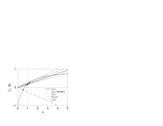
FIG. 4.: Graphical construction of the solutions of $\lambda_{s}=s\gamma$ for different values of $\gamma$ at dissipation $\alpha=0.5$. Intersections $(s_{0})$ with smaller $s-$values are marked with filled circles, and intersections $(s_{1})$ with larger $s-$values with open ones.

To study the long time approach of $\tilde{f}(c,t)$ to the scaling solution $\tilde{f}(c)$ in (I.1), we analyze the approach of the rescaled moments $\mu_{n}(t)=m_{n}(t)/e^{n}_{o}(t)$ to the moments $\mu_{n}$ of the scaling solution $\tilde{f}(c)$. To do so we have to choose $\gamma=\lambda_{1}$ (see Fig.4) on account of (II.5) and (II.14). The infinite set of moment equations (IV.6) for $\mu_{n}(t)$ can be solved sequentially for all $n$ as an initial value problem. To explain what is happening, it is instructive to use a graphical method to determine the zeros of the eigenvalue $\gamma_{s}=\lambda_{s}-s\gamma$ for different values of $\gamma$. This is illustrated in Fig.4 by determining the intersections $\{s_{0},s_{1}\}$ of the curve $y=\lambda_{s}$ and the line $y=s\gamma$, where $s_{0}$ and $s_{1}$ are denoted respectively by filled ($\bullet$) and open circles ($\circ$). These circles divide the spectrum into a (linearly) stable branch ($s_{0}<s<s_{1}$) and two unstable branches ($s<s_{0}$) and ($s>s_{1}$). The moments $\mu_{s}(t)$ with $s=n>a$ are on an unstable branch $(\gamma_{s}<0)$ and will grow for large $t$ at an exponential rate, $\mu_{n}(t)\simeq\mu_{n}(0)\exp[|\gamma_{n}|t]$, as can be shown by complete induction from (IV.6) starting at $n=[a]+1$. They remain positive and finite for finite time $t$, but approach $+\infty$ as $t\to\infty$, in agreement with the predictions of the self consistent method of Sect.III. The moments with $n$ on the stable branch are linearly stable ($\gamma_{n}>0$), but may still grow through nonlinear couplings with lower moments $\mu_{l}(t)$ whenever $l=1,2,\cdots$ is on the unstable branch ($l<s_{0}$). This is relevant for the discussion in the next subsection. In the case $\gamma=\lambda_{1}$ under consideration however, all moments $\mu_{l}$ with $l=1,2,\cdots,[a]$ are globally stable and approach for $t\to\infty$ the limiting value $\mu_{n}(\infty)=\mu_{n}$, which are the finite positive moments of the scaling form (IV.2), plotted in Fig.3.

The behavior of the moments described above is considered as a weak form of convergence or approach of $\tilde{f}(c,t)$ to $\tilde{f}(c)$ for $t\to\infty$. This result will be described in a more precise form and summarized in the last section. The physically most relevant distribution functions $f(v,t)$ and rescaled distribution functions $\tilde{f}(c,t)$ are those with regular initial conditions, i.e. all moments $m_{n}(0)=e^{n}_{o}(0)\mu_{n}(0)<\infty$. This implies that the initial condition for the rescaled Fourier transform $\tilde{\phi}(x,0)$ with $x=\textstyle{\frac{1}{4}}k^{2}$ of $\tilde{f}(c,0)$ has a series expansion regular at the origin $x=0$, i.e. all its derivatives exist in that point.

C More similarity solutions

The results of the previous subsection can also be generalized to different values of $\gamma$ and different classes of initial distributions, which possess only a finite set of bounded moments $m_{n}(0)$. Here we summarize only the most important results of these generalizations, the details of which will be published elsewhere [39].

The case, $\gamma>\lambda_{1}$, concerns the line $y=s\gamma_{2}$ in Fig.4. Then $\mu_{1}(t)$ will always be in the unstable region (there is either an intersection point $s_{0}>1$, or there are no intersection points at all). So, $\mu_{1}(t)\to\infty$ as $t\to\infty$ at an exponential rate, and it drives all moments $\mu_{n}(t)\to\infty$ through nonlinear couplings to $\mu_{1}(t)$, which is present on the right hand side of (IV.6). Consequently, there is no approach to the scaling form $\Phi(x)$ with a rate constant $\gamma>\lambda_{1}$.

The case, $0<\gamma<\lambda_{1}$, concerns the line $y=s\gamma_{4}$ where there are two intersection points $\{s_{0},s_{1}\}$ with $s_{0}=a<1$ and $s_{1}=b>1$, corresponding to the dominant singularity $x^{a}$ and a subleading singularity $x^{b}$. The dominant singularity corresponds to a power law tail $\tilde{f}(c)\sim 1/c^{2a+d}$ with $a<1$. Because $a<1$, the system has infinite energy at all times. All higher moments $\mu_{n}$ with $n=2,3,\dots$ are divergent as well at all times. Consequently, the initial states under discussion are already singular with $\phi(x,0)\simeq 1-Ax^{a}$. Of course such states are of much less interest for possible physical applications than the regular ones, discussed in the previous subsection. The feature of interest here is to demonstrate that inelastic Boltzmann equations generate for initial states characterized by a singularity $x^{a}$ with $a<1$ a new type of singularity $x^{b}$, which is found through the graphical construction using line $y=s\gamma_{4}$. For elastic Maxwell molecules such states have been analyzed recently by Bobylev and Cercignani [31]. In one-dimensional systems these initial states are closely related to Levy distribution [40] with the characteristic function $\varphi(k)=\exp[-bk^{2a}]$, where $b$ is positive. For such distributions it is well known that Fourier inversion yields for $0<a<1$ a non-negative distribution $f(v)$ with a power law tail $1/v^{2a+d}$ with $d=1$. On the other hand, for $a>1$ Fourier inversion may lead to a distribution with negative $f(v)$.

However, in this case one can say more. Following Bobylev and Cercignani, we assume that we can construct a non negative initial distribution with a $\phi(x,0)$ which is a regular function of $\zeta=x^{a}$ in a neighborhood of $\zeta=0$, i.e.

$$\phi(x,0)=\sum_{n=0}^{\infty}(-1)^{n}\frac{x^{na}}{n!}A_{n}(0),$$ (IV.8)

where $|A_{n}(0)|<A^{n}$, and we have chosen normalization such that $A_{0}(0)=A_{1}(0)=1$. We have slightly modified the example of [31] to have a finite non-vanishing radius of convergence of (IV.8). Then we can demonstrate that the rescaled characteristic function $\tilde{\phi}(y,t)\equiv\phi(x,t)$ approaches in the scaling limit ($t\to\infty$ with $y\equiv x\exp[-\gamma t]$ fixed) a positive scaling form or similarity solution $\Phi(y)$ with $\gamma=\lambda_{a}/a$, and

$$\Phi(y)=\sum_{n=0}^{[b]}(-1)^{n}\frac{x^{na}}{n!}A_{n}(\infty)+o(y^{b}),$$ (IV.9)

where $A_{0}(\infty)=A_{1}(\infty)=1$. The approach is again in the weak sense of a finite set of moments. The $A_{n}(\infty)$ are positive and can be calculated from a set of recursion relations, rather similar to (IV.3). Moreover, $b=s_{1}$ is the left most intersection point of $\lambda_{s}$ with the line $y=s\gamma_{5}$ (see the left most open circle on $\lambda_{s}$). So, the initial $\phi(x,0)$, which is regular in $\zeta=x^{a}$ around $\zeta=0$, develops a new singularity of the type $x^{b}$. This can again be demonstrated by considering the rescaled function $\tilde{\phi}(y,t)$, defined as $\phi(x,t)=\tilde{\phi}(e^{-\gamma t}y,t)$, and expanding $\tilde{\phi}(y,t)$ in a series like (IV.8) with $A_{n}(0)$ replaced by $A_{n}(t)$. The coefficients satisfy moment equations, rather similar to (IV.6).

In the case, $\gamma\leq 0$, the results are similar to those in the previous paragraph, except that there is only one intersection point at $s_{0}=a$ (see the line $y=s\gamma_{5}=-|\gamma_{5}|s$). The energy and all higher moments are infinite, and the scaling form of the characteristic function $\Phi(x)$ is a regular function of $\zeta=x^{a}$ near the origin. A similar solution for the elastic case has been obtained in Ref. [31].

V Conclusions

Using self consistency arguments we have shown that the nonlinear Boltzmann equation for the inelastic Maxwell models IMM-A and IMM-B admits a scaling solution $\tilde{f}(c)$ with a power law tail $1/c^{2a+d}$ where the exponent $a$ is given by the root $a$ with $a>1$ of a transcendental equation. This implies that all moments $\mu_{n}$ of $\tilde{f}(c)$ are divergent for $n>a$, and those $\mu_{n}$ with $n<a$ are positive and finite, and are given recursively through (IV.3) with initialization $\mu_{1}=1$.

For systems with dissipative dynamics we have formulated a conjecture about the long time approach, for general classes of initial distributions, of the rescaled distribution function $\tilde{f}(c,t)=v^{d}_{o}(t)f(cv_{o}(t),t)$ to a scaling solution $\tilde{f}(c)$ with an high energy tail, which is overpopulated when compared to a Gaussian distribution. For the inelastic Maxwell models, studied in detail in this article, we have demonstrated this approach to the scaling solution $\tilde{f}(c)$ in subsection IV.B in the following weak sense:
Given on the one hand the rescaled moments $\mu_{n}(t)=m_{n}(t)/e^{n}_{o}(t)$ of the physically most relevant class of regular initial distributions with all moments $m_{n}(0)$ bounded, and rescaled according to (I.1), and given on the other hand the unique set of finite positive moments $\mu_{n}$ of the scaling form with $n<a$, then all $\mu_{n}(t)$ with $n<a$ approach for $t\to\infty$ the limiting value $\mu_{n}$ through a sequences of positive numbers, and all moments $\mu_{n}(t)$ with $n>a$ behave as $\mu_{n}(t)\simeq\mu_{n}(0)\exp[|\gamma_{n}|t]\to+\infty$ as $t\to\infty$. This is in agreement with all known properties of the scaling solution.

We consider the long time behavior of the set of moments $\mu_{n}(t)\to\mu_{n}\;\;(n<a)$ and $\mu_{n}(t)\to+\infty\;\;(n>a)$ as a demonstration that $\tilde{f}(c,t)$ approaches the scaling form $\tilde{f}(c)$ for $t\to\infty$. We further note that these results for the long time behavior of inelastic Maxwell models, after the rescaling of the initial distribution, are universal, i.e. they are independent of all details of the initial distributions. We consider the present results for inelastic Maxwell models as strong support for our more general conjecture, which is also confirmed for inelastic Maxwell models through the Monte Carlo simulations of the Boltzmann equation by Baldassarri et al, in which the approach of $\tilde{f}(c,t)$ to a positive power law tail with the predicted exponent $a$ was confirmed within reasonably small error bars.

Appendix A: Angular averages in d-dimensions

The angular average (III.7) of powers of $\hat{\bf a}\cdot{\bf n}=\cos\theta$ can be simply calculated by using polar coordinates with $\hat{\bf a}$ as the polar axis. Then,

$$\beta_{s}=\int_{\bf n}|\hat{\bf a}\cdot{\bf n}|^{s}=\frac{\int_{0}^{\pi}d\theta(\sin\theta)^{d-2}(\cos\theta)^{s}}{\int_{0}^{\pi}d\theta(\sin\theta)^{d-2}}=\frac{\Gamma(\frac{s+1}{2})\Gamma(\frac{d}{2})}{\Gamma(\frac{s+d}{2}\Gamma(\frac{1}{2})}.$$ (A.1)

For $s=2n$ this formula can be expressed as

$$\beta_{2n}=(1/2)_{n}/(d/2)_{n},$$ (A.2)

where the Pochhammer symbol is defined as

$$(a)_{n}=\Gamma(a+n)/\Gamma(a)=a(a+1)\dots a(a+n-1).$$ (A.3)

In fact, we will use the notations $(a)_{s}$, $\beta_{2s}$, $s!=(1)_{s}$ and $\left(\begin{array}[]{c}s\\ r\end{array}\right)$ also for non-integer values of $s$ by expressing these quantities in terms of Gamma functions.

Next we define $H(l,m)$ and $\lambda_{n}$, introduced in (IV.1) for model IMM-A,

$$H(l,n-l)=\left(\begin{array}[]{c}n\\ l\end{array}\right)\displaystyle\int_{\bf n}e_{+}^{l}({\bf n})e_{-}^{n-l}({\bf n})$$ (A.6)

$$\lambda_{n}=1+\delta_{n0}-H(0,n)-H(n,0)=\displaystyle\int_{\bf n}[1+\delta_{n0}-e_{+}^{n}({\bf n})-e_{-}^{n}({\bf n})],$$ (A.7)

where $e_{\pm}({\bf n})$ has been defined in (III.3). For model IMM-B one needs to replace $\int_{\bf n}$ with $\int^{\prime}_{\bf n}|\hat{a}\cdot{\bf n}|$. These expressions hold for $d=1,2,....$. Evaluation of $H(l,m)$ requires,

$$I(m,n)=\int_{\bf n}e_{+}^{m}e_{-}^{n}=\frac{2p^{2m}}{B(\frac{d-1}{2},\frac{1}{2})}\int_{0}^{\pi/2}d\theta(\sin\theta)^{d-2}(\cos\theta)^{2m}[1-z\cos^{2}\theta]^{n},$$ (A.8)

where $z=1-(1-p)^{2}$. Following Krapivsky and Ben-Naim [23] we change to the new integration variable $\mu=\cos^{2}\theta$, to find for $d=1,2,\dots$

$$H(m,n) = \left(\begin{array}[]{c}n+m\\ m\end{array}\right)\frac{p^{2m}}{B(\frac{d-1}{2},\frac{1}{2})}\int_{0}^{1}d\mu\mu^{m-1/2}(1-\mu)^{\frac{d-3}{2}}[1-z\mu]^{n}$$ (A.11)

$$= \left(\begin{array}[]{c}n+m\\ m\end{array}\right)\beta_{2m}p^{2m}\,_{2}F_{1}(-n,m+\frac{1}{2},m+\frac{d}{2};z)$$ (A.14)

$$= p^{2m}\left(\begin{array}[]{c}n+m\\ m\end{array}\right)\sum_{l=0}^{n}\left(\begin{array}[]{c}n\\ l\end{array}\right)\beta_{2l+2m}(-z)^{l}.$$ (A.19)

On the second and third line we have used the fundamental integral representation for the hyper-geometric function $\ {}_{2}F_{1}$, and its Gauss series, i.e.

$$\,{}_{2}F_{1}(a,b,c;z)=\left\{\begin{array}[]{l}B^{-1}(b,c-b)\int_{0}^{1}dtt^{b-1}(1-t)^{c-b-1}(1-zt)^{-a}\\[5.69054pt] \sum_{l=0}^{\infty}\frac{(a)_{l}(b)_{l}}{(c)_{l}l!}z^{l}.\end{array}\right.$$ (A.22)

When $a=-n,\,(n=0,1,2\dots)$, then $\,{}_{2}F_{1}(-n,b,c;z)$ is a polynomial of degree $n$ in $z$, and the Gauss series ends at $l=n$.

To calculate the eigenvalue $\lambda_{n}$ in (A.6) we deduce from (A.22)

$$H(n,0) = \beta_{2n}p^{2n}$$ (A.23)

$$H(0,n) = \,{}_{2}F_{1}(-n,\frac{1}{2},\frac{d}{2};z)=\sum_{l=0}^{n}\left(\begin{array}[]{c}n\\ l\end{array}\right)\beta_{2l}(-z)^{l}.$$ (A.26)

REFERENCES

- [1] G.P. Collins, A Gas of Steel Balls, Sci. Am. 284, vol.1, 17 (2001) .
- [2] C.S. Campbell, Annu. Rev. Fluid Mech. 22, 57 (1990).
- [3] N. Sela and I. Goldhirsch, Phys. Fluids 7, 507 (1995).
- [4] T. P. C. van Noije and M. H. Ernst, Granular Matter 1 (1998) 57, and cond-mat/9803042.
- [5] Th. Biben, Ph. A. Martin and J. Piasecki, preprint July 2001.
- [6] A. Barrat, T. Biben, Z. Racz, E. Trizac and F. van Wijland, cond-mat/0110345.
- [7] J.J. Brey, M.J. Ruiz-Montero and D. Cubero, Phys. Rev. E 54, 3664 (1996).
- [8] J. M. Montanero and A. Santos, Granular Matter 2, 53 (2000), and cond-mat/0002323.
- [9] M. Huthmann, J.A.G. Orza and R. Brito, Granular Matter 2, 189 (2000), and cond-mat/0004079.
- [10] T.P.C.van Noije, M.H.Ernst, E.Trizac and I. Pagonabarraga, Phys. Rev. E 59, 4326 (1999). I.Pagonabarraga, E.Trizac, T.P.C.van Noije and M.H. Ernst, cond-mat/0107570.
- [11] S. E. Esipov and T. Pöschel, J. Stat. Phys. 86, 1385 (1997).
- [12] E. Ben-Naim and P. Krapivsky, Phys. Rev. E 61, R5 (2000).
- [13] A. V. Bobylev, J. A. Carrillo, I. M. Gamba, J. Stat. Phys. 98, 743 (2000).
- [14] J. A. Carrillo, C. Cercignani, and I. M. Gamba, Phys. Rev. E 62, 7700 (2000).
- [15] C. Cercignani, J. Stat. Phys. 102, 1407 (2001).
- [16] A. Bobylev and C. Cercignani, J. Stat. Phys. 106, 547 (2002).
- [17] R.S. Krupp, A non-equilibrium solution of the Fourier transformed Boltzmann equation, M.S. dissertation, M.I.T., Cambridge, Mass. (1967).
- [18] A. V. Bobylev, Sov. Phys. Dokl. 20, 820 (1975), A. V. Bobylev, Sov. Phys. Dokl. 21, 632 (1976).
- [19] T. Krook and T.T. Wu, Phys. Rev. Lett. 36, 1107 (1976).
- [20] M. H. Ernst, Physics Reports 78, 1 (1981).
- [21] A. Baldassarri, U. Marini Bettolo Marconi and A. Puglisi, cond-mat/0111066, 5 Nov 2001.
- [22] A. Baldassarri, private communication.
- [23] P. Krapivsky and E. Ben-Naim, cond-mat/0111044, 2 Nov 2001, and cond-mat/0202332, 20 Febr 2002.
- [24] M.H. Ernst and R. Brito, cond-mat/0111093, 6 Nov. 2001, and Europhys. Lett., 58, 182 (2002).
- [25] M.H. Ernst and R. Brito, Phys. Rev. E 65, 040301(R) (2002).
- [26] B. Nienhuis, private communication, September 2001.
- [27] I. Goldhirsch and G. Zanetti, Phys. Rev. Lett. 70, 1619 (1993).
- [28] P.K. Haff, J. Fluid Mech. 134, 40 (1983).
- [29] J.J. Brey, J.W. Dufty and A. Santos, J. Stat. Phys. 87, 1051 (1997).
- [30] A. Baldassarri, U. Marini Bettolo Marconi and A. Puglisi, cond-mat/0105299, 15 May 2001.
- [31] A. Bobylev and C. Cercignani, Exact eternal solutions of the Boltzmann equation, (see http://www.math.tu-berlin.de/tmr/preprint/d.html).
- [32] A. Bobylev and C. Cercignani, J. Stat. Phys. 106, 1039 (2002).
- [33] P. Résibois and M. de Leener, Classical Kinetic Theory of Fluids (Wiley, New York, 1977).
- [34] C. Cercignani, The Boltzmann equation and its applications (Springer Verlag, New York, 1988).
- [35] D. Ruelle, J. Stat. Phys. 95 (1999) 393.
- [36] D.J. Evans and L. Rondoni, Comments on the Entropy of Nonequilibrium Steady States, J. Stat. Phys, this issue.
- [37] J. R. Dorfman, An Introduction to Chaos in Nonequilibrium Statistical Mechanics, Cambridge Lecture Notes in Physics, Vol 14, section 13.4 (Cambridge University Press, 1999).
- [38] A. Bobylev and C. Cercignani, private communication.
- [39] M.H. Ernst and R. Brito, in preparation.
- [40] E.W.Montroll and B.J. West, On an enriched collection of Stochastic processes, Fluctuation Phenomena, edited by E.W. Montroll and J.L. Lebowitz (North Holland, Amsterdam, 1979).