Landau-Zener transitions in a linear chain.

Abstract

We present an exact asymptotic solution for electron transition amplitudes in an infinite linear chain driven by an external time-dependent electric field. This solution extends the Landau-Zener theory for the case of an infinite number of states in the discrete spectrum. In addition to the transition amplitudes we calculate the effective diffusion constant.

Landau-Zener (LZ) theory landau ,zener treats a quantum system placed in a slowly varying external field. If such a system was prepared in a state of its discrete spectrum, it adiabatically follows this state until its time dependent energy level crosses another one. Near the crossing point the adiabaticity can be violated and the system can escape from the state it occupied initially to another one. Landau and Zener found the transition probability for two-level crossing. The crossing of more than two levels at the same time is generally an unlikely coincidence. However, in some systems such a multi-level crossing may occur systematically, due to the high symmetry of the underlying Hamiltonian. The transition matrix for special cases of multi-level crossing was studied in Refs. zeeman1 ; zeeman2 ; bow ; demkov ; deminf1 ; elser . Presently only a few exact results for multi-level crossing are known. One of them relates to a multiplet of atomic electronic states with a total spin $S$ or total rotational moment $J$ larger than 1/2 in a varying external magnetic field zeeman1 ; zeeman2 . The Zeeman splitting between $2S+1$ or $2J+1$ levels regularly vanishes at nodes of the magnetic field. Another exactly solvable model displaying multi-level crossing is the so-called bow-tie model bow , whose physical interpretation is not obvious.

Since its creation in 1932, LZ theory has had numerous applications. They include molecular pre-dissociation LL , slow atomic and molecular collisions collisions , and electron transfer in biomolecules biomolecules . Recently Wernsdorfer et al. WS1 ,WS2 employed the LZ theory to describe consistently the step-like shape of the hysteresis loop in special molecules with large magnetic moments called nano-magnets. Using the LZ probability formula these authors were able to find the extremely small tunnel splitting of the classic degenerate ground states and even to reveal oscillations of this value in external magnetic field. This beautiful experiment, together with its clever treatment is a new triumph of quantum mechanics and, in particular LZ theory.

The problem considered in this article is closely related to another application of LZ theory: electronic transfer in donor-acceptor complexes vol . In this process of biological and chemical importance, an electron tunnels between initial and final positions through a long chain of identical sites. There are two limiting cases for such a process. In the first case there is no coherence between two sequential tunnelling processes connecting nearest neighbor sites. In this case the probability of tunnelling through several sites is very small in comparison to that for one-site tunnelling. This limiting case was studied earliervol . We consider the opposite limiting case in which the sequential tunnelling processes are highly coherent and tunnelling through many sites becomes available.

If the coherence between LZ transitions is lost, the problem is reduced to multiplication and addition of probabilities, each described by a proper LZ expression. The price we must pay for incorporating the coherence between different transitions is a strong reduction of the class of quantum systems considered. The number of crossing levels in such systems must be infinite. The hopping amplitudes from a site to its neighbors must be all identical. Physically it describes the quantum electron transfer between donor and acceptor separated by a long polymer strand (molecular bridge). The bridge can be considered as a linear array of identical sites. Such one-dimensional atomic-scale wires were intensely studied, both experimentally and theoretically wire ; wire1 ; wire2 . Our result can be also applied to transitions among electron states in semiconductor superlattices sl1 ; sl2 .

We study the tunnelling of a particle in such systems driven by a time-dependent homogeneous external field. An important assumption is that all molecular fragments in the chain are identical. An electric field splits the energy levels at different sites of the chain and suppresses the transitions, which occur within a narrow intervals about times when the electric field becomes zero. Since the tunnelling is a fast process, we disregard the oscillatory relaxation originating from phonons and other elementary excitations.

Let denote $|n>$ a state located at the $n$-th site of the chain. We assume that these states form a complete orthonormal set (Wannier basis). In terms of this set the electron Hamiltonian reads:

$$\hat{H}=\sum\limits_{n=1}^{N}(\gamma\mid n\rangle\langle n+1\mid+c.c.)+F(t)n\mid n\rangle\langle n\mid;$$ (1)

$$F(t)=eE(t)a$$

where $E(t)$ is the electric field, $e$ is the electron charge, $a$ is the distance between sites and $\gamma$ is the coupling constant (hopping amplitude). A series of exact solutions for the time-dependent Shrödinger equation with the Hamiltonian (1) for $N=\infty$, known as drifting plane waves, was found long ago sl2 ; bloch ; wannier ; dev ; hid . Below we solve the same problem for fixed initial conditions, thus resolving the multi-state LZ problem.

The states $|n>$ are conventionally called the diabatic states. They are the eigenstates of the diagonal part of this Hamiltonian $H_{0}=F(t)n\mid n\rangle\langle n\mid$. The eigenstates of the total Hamiltonian (1) depending on $t$ or $F(t)$ as parameters are called adiabatic states. Until $\mid F(t)\mid\gg\gamma$, the diabatic levels are close to the adiabatic ones and the transitions between levels are suppressed. This is the adiabatic regime. The adiabaticity is violated in the vicinity of the electric field nodes determined by the inequality $\mid F(t)\mid\leq\gamma$, where all transitions proceed. By level crossing we mean that the diabatic levels cross, the exact eigenvalues of the Hamiltonian (1) never cross, in accordance to the Wigner - Neumann theorem. It is convenient to place the time origin $t=0$ directly at the node of $F(T)$. Since only a narrow vicinity of the node is substantial for transitions, the exact dependence of the field on time can be reasonably approximated by linear one: $F(t)\approx\dot{F}(0)\cdot t$. At zero electric field $E$ and free boundary conditions the Hamiltonian (1) can be diagonalized analytically. Its spectrum is:

$$\varepsilon_{j}=2g\cos(\pi j/N);\,\,\,\,j=1\ldots N$$ (2)

For non-zero field we have found the adiabatic eigenvalues numerically. The result is shown in Fig. 1 for a finite chain with 15 sites. For comparison the diabatic levels are depicted in the same figure.

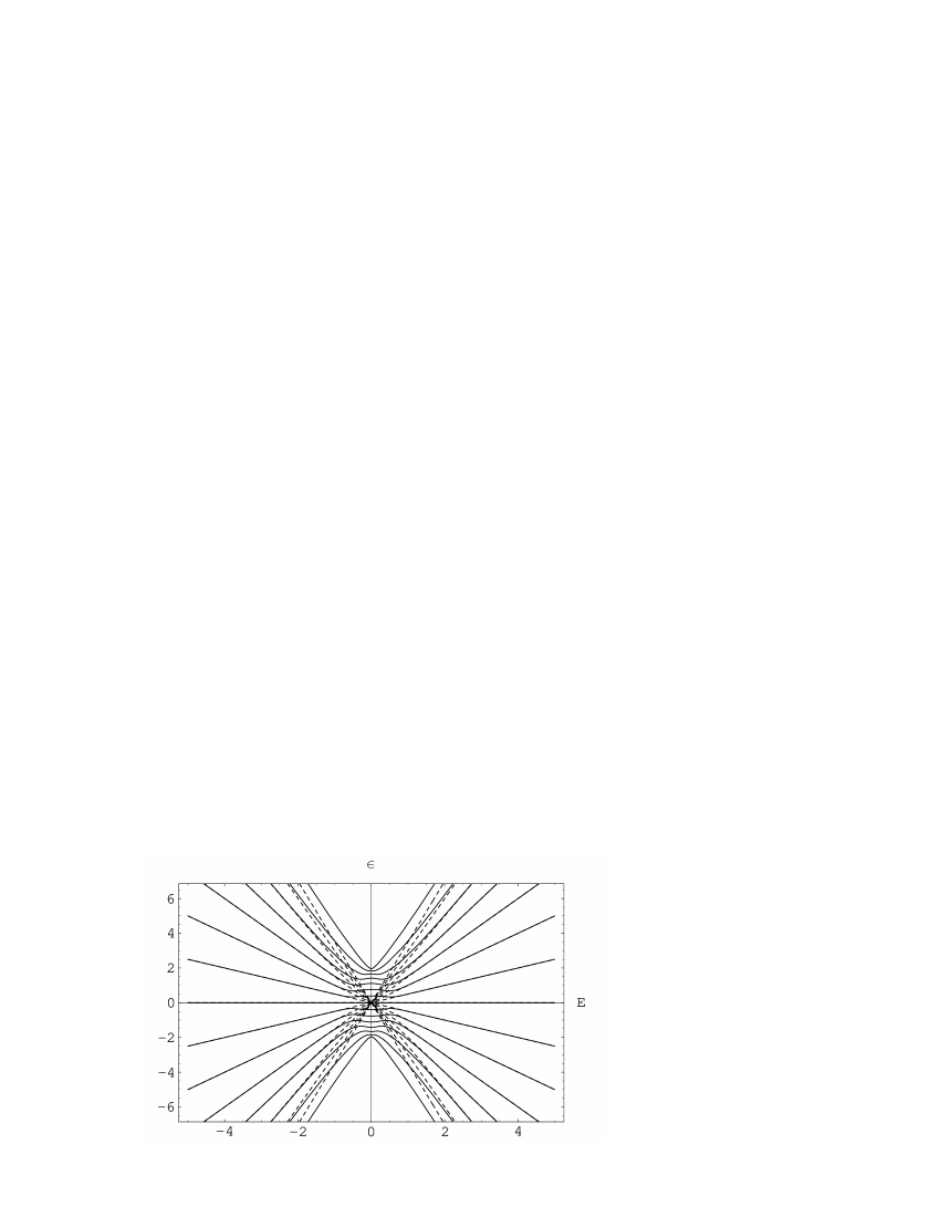
Figure 1: Dependence of eigenvalues of the Hamiltonian (1) on $E$. Solid lines show adiabatic energies as function of $E$, dashed lines depict diabatic energies. While the diabatic levels intersect in one point, the adiabatic levels do not intersect.

We proceed to solve the time-dependent Schrödinger equation with the Hamiltonian (1). Its matrix representation reads:

$$H_{nm}=n\dot{F}(0)t\delta_{nm}+\gamma(\delta_{m,n+1}+\delta_{m,n-1})$$ (3)

For an infinite chain ($N\rightarrow\infty$) equation (3) is valid for all $n$ and $m$. After a proper rescaling of time the Hamiltonian (3) becomes dimensionless:

$$H_{mn}=nt\delta_{mn}+g(\delta_{m,n+1}+\delta_{m,n-1})$$ (4)

It depends on only one dimensionless number, $g=\gamma/\sqrt{\dot{F}(0)}$, which is the Landau-Zener parameter. Let the time-dependent state vector be $\mid\alpha,t\rangle=\sum_{n}c_{n}(t)\mid n\rangle$. Then the system of equations for the amplitudes $c_{n}(t)$ reads:

$$i\dot{c}_{n}=ntc_{n}+g(c_{n-1}+c_{n+1})$$ (5)

The transition matrix element $T_{n,n^{\prime}}$ should be identified with the $t\rightarrow+\infty$ asymptote of an amplitude $c_{n}(t)$ for a solution obeying the initial condition $|c_{m}(t)|^{2}=\delta_{m,n^{\prime}}$ at $t\rightarrow-\infty$. Since all $c_{m}(t)$ except of $c_{n}^{\prime}(t)$ are zero at $t\rightarrow-\infty$, the initial condition can be more explicitly written as

$$c_{m}(t\rightarrow-\infty)=\delta_{m,n^{\prime}}\exp{(-in^{\prime}t^{2}/2)}$$ (6)

We multiply the asymptotic values of $c_{n}(t)$ by $\exp{[int^{2}/2]}$ to remove strongly oscillating phase factors from $T_{n,n^{\prime}}$.

Now introduce an auxiliary function $u(\varphi,t)=\sum_{n=-\infty}^{\infty}c_{n}(t)e^{in\varphi}$. The system (5) is equivalent to the following equation in partial derivatives for $u(\varphi,t)$:

$$\frac{\partial u}{\partial t}+t\frac{\partial u}{\partial\varphi}+2igu\cos\varphi\,=\,0$$ (7)

The initial condition (6) is equivalent to the initial condition: $u(\varphi,t\rightarrow-\infty)\rightarrow\exp[in^{\prime}(-\frac{t^{2}}{2}+\varphi)]$. Given the solution $u(\varphi,t)$, the amplitudes $c_{n}(t)$ can be found by the inverse Fourier transformation $c_{n}(t)=\frac{1}{2\pi}\int_{0}^{2\pi}u(\varphi,t)e^{-in\varphi}d\varphi$. The solution of eq. (7) that obeys proper boundary conditions is:

$$u(\varphi,t)=\exp\left[-i\left(2g\int\limits_{-\infty}^{t}\cos\left(\varphi-\frac{t^{2}}{2}+\frac{t^{{}^{\prime}2}}{2}\right)dt^{{}^{\prime}}+\right.\right.$$

$$\left.\left.n^{{}^{\prime}}\left(\varphi-\frac{t^{2}}{2}\right)\right)\right]$$ (8)

Putting $t=+\infty$ in the solution (8) and taking the inverse Fourier-transform, we arrive at following asymptotic values:

$$c_{n}(t)\approx\exp\left(-\frac{int^{2}}{2}+i\frac{(n^{\prime}-n)\pi}{4}\right)J_{|n-n^{\prime}|}(2\sqrt{2\pi}g)$$ (9)

Thus, the scattering amplitudes in terms of modified states, with the fast phase factor $\exp(-int^{2}/2)$ incorporated, are:

$$T_{n,n^{\prime}}\equiv\langle n\mid T\mid n^{\prime}\rangle=e^{i(n^{\prime}-n)\pi/4}J_{|n-n^{\prime}|}(2\sqrt{2\pi}g),$$ (10)

where the operator $T$ is expressed in terms of the evolution operator $U(t,t^{\prime})$ for the Hamiltonian (4) in the interaction representation:

$$T=\lim_{t\rightarrow\infty;\,t^{\prime}\rightarrow-\infty}\exp(i\int_{t^{\prime}}^{0}H_{0}(\tau)d\tau)U(t,t^{\prime})\exp(i\int_{0}^{t}H_{0}(\tau)d\tau)$$ (11)

The matrix elements $T_{n,n^{\prime}}$ display an infinite number of oscillations with the LZ parameter $g$. However, for large $|n-n^{\prime}|$ the oscillations start with $g>|n-n^{\prime}|$. These oscillations can be observed experimentally by varying the field sweep rate $\dot{E}(0)$. For small values of $g$ the amplitudes are small and quickly decrease with growing $|n-n^{\prime}|$. In Fig. 2 we depict transition probabilities for several levels $n$ closest to the initial one $n^{\prime}$ versus the Landau-Zener parameter $g$. Fig. 3 shows the dependence of the transition amplitude on $\mid n-n^{\prime}|$ at a fixed value of $g$.

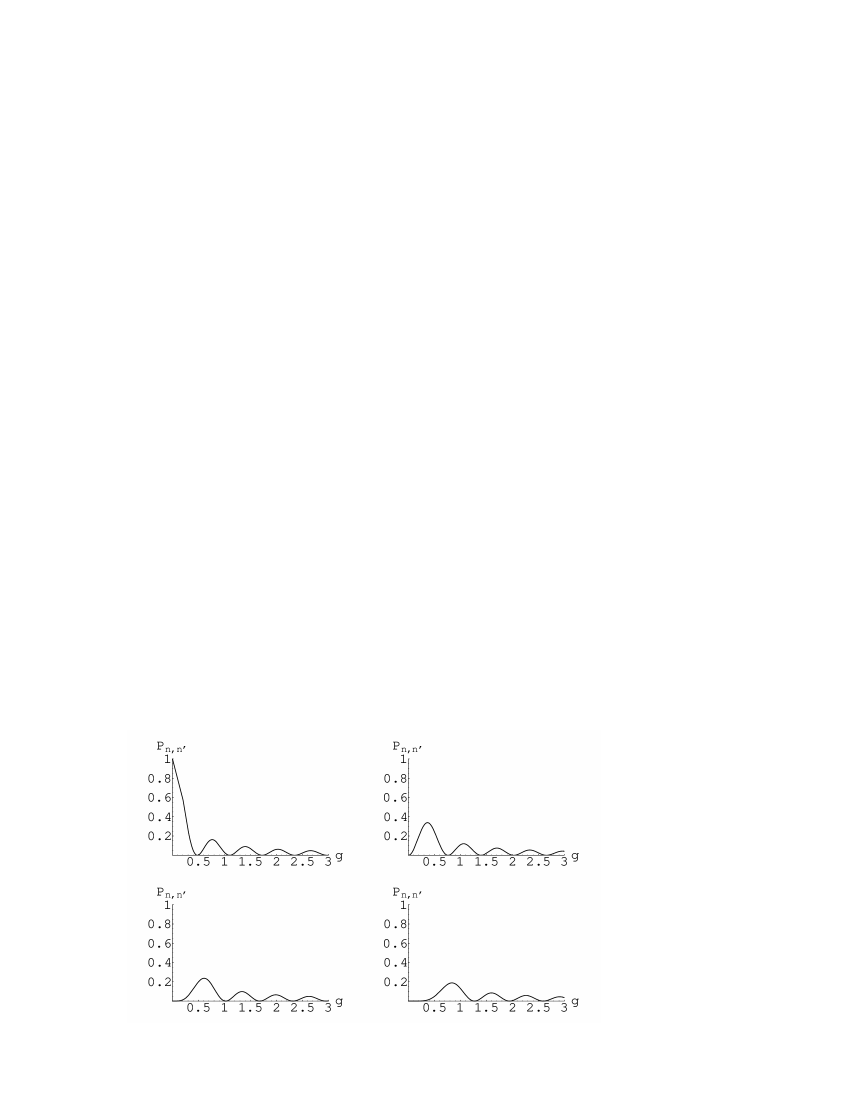
Figure 2: Transition probabilities to sites closest to an initially filled one as functions of $g$: (a) $|n-n^{\prime}|=0$; (b) $|n-n^{\prime}|=1$; (c) $|n-n^{\prime}|=2$; (d) $|n-n^{\prime}|=3.$

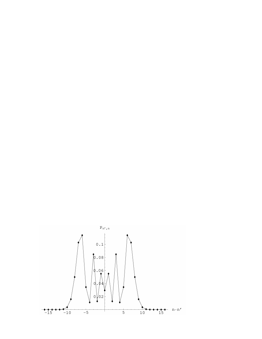
Figure 3: Transition probabilities vs. $n-n^{\prime}$ at a fixed $g=1.6.\,Solid\,line\,is\,a\,guide\,for\,eye.$

For large $g\gg|n-n^{\prime}|$ the asymptotic values of the amplitudes (10) are:

$$\langle n\mid T\mid n^{\prime}\rangle\sim\frac{e^{i(n^{\prime}-n)\pi/4}}{(\sqrt{2\pi^{3}}g)^{1/2}}\cos(2\sqrt{2\pi}g-\frac{(n-n^{\prime})\pi}{2}-\frac{\pi}{4})$$ (12)

It is instructive to compare this result with other exactly solvable generalized Landau-Zener models. Most of them refer to systems with a finite number of states $N$. In the limit $g\gg N$ the transition probabilities behave like an exponent $\exp(-C(n,n^{\prime})g^{2})$, where the $C(n,n^{\prime})$ do not depend on $g$. In contrast, the result (12) displays a power law with oscillations instead of an exponential dependence on $g$ for large $g$. This is the manifestation of quantum interference of different Feynman trajectories, which are discrete in the chain. A step in a trajectory has average length $g$ (see below). Such a step cannot be realized in a system with a finite number of states if $g\gg N$.

The mean square displacement at one crossing event is:

$$<(n-n^{\prime})^{2}>=\sum\limits_{n=-\infty}^{\infty}(n-n^{\prime})^{2}|J_{|n-n^{\prime}|}(2\sqrt{2\pi}g)|^{2}=$$

$$=4\pi g^{2}$$ (13)

If the external field is periodic in time and the coherence between crossing events is lost, the electron performs a random walk, i.e. it diffuses. Assume the field to oscillate harmonically as $F(t)=F_{0}\sin(\omega t)$. At the nodes $t_{k}=\pi k/\omega$ ($k$ is an integer) all diabatic levels cross together. The squared Landau-Zener parameter is $g^{2}=\frac{\gamma^{2}}{F_{0}\omega}$. The diffusion coefficient is $D=2a^{2}<(n-n^{\prime})^{2}>/T$, where $T=2\pi/\omega$ is the period of oscillations and the factor $2$ accounts for two crossing events per period. Collecting these results and equation (13), we find:

$$D=\frac{4a\gamma^{2}}{F_{0}}$$ (14)

This result does not depend on the frequency of the external field.

The theory can be extended to a more general Hamiltonian incorporating hopping between any two sites, but conserving translational invariance:

$$H=\sum_{m,n}H_{m,n}|m\rangle\langle n|;$$

$$H_{mn}=nt\delta_{mn}+g_{|m-n|};\quad g_{-k}=g_{k}^{*}$$ (15)

For simplicity we present below the result for real hopping amplitudes $g_{k}=g_{-k}$:

$$\left\langle n\right|T\left|n^{{}^{\prime}}\right\rangle=\frac{e^{i(n^{\prime}-n)\pi/4}}{2\pi}\int\limits_{0}^{2\pi}\exp\left(-i2\sqrt{2\pi}f(\varphi,g_{j})\right.$$

$$\left.+i(n^{{}^{\prime}}-n)\varphi\right)d\varphi$$ (16)

where $f(\varphi,g_{j})=\sum\nolimits_{k}\frac{g_{k}}{\sqrt{k}}\cos k\varphi$.

The model (1) can be generalized also to incorporate internal degrees of freedom of identical chain fragments. In this case the local states are described by amplitudes $a_{n,\alpha}$ with two indices. The first index $n$ denotes the position and the second index $\alpha$ labels the inner states. The Schrödinger equation for the amplitudes then reads:

$$i\dot{a}_{n,\alpha}=(nt+{\epsilon}_{\alpha}+{\delta}_{\alpha}t)a_{n,\alpha}+\sum\limits_{\beta}g_{\alpha,\beta}(a_{n+1,\beta}+a_{n-1,\beta})$$ (17)

where the indexes $\alpha,\beta=1\ldots N_{int}$ run over the internal states of the molecular wire segment. Changing to variables $a_{n,\alpha}=b_{n,\alpha}e^{-int^{2}/2}$ we eliminate the term proportional to $t$ in equation (17). Introducing a new function $u_{\alpha}(\varphi)=\sum_{n=-\infty}^{\infty}b_{n,\alpha}e^{in\varphi}$, we reduce the infinite system (17) to a finite set of $N_{int}$ ordinary differential equations:

$$i\dot{u}_{\alpha}=(\epsilon_{\alpha}+{\delta}_{\alpha}t)u_{\alpha}+2\cos(t^{2}+\varphi)\sum\limits_{\beta}g_{\alpha,\beta}u_{\beta}$$ (18)

in which $\varphi$ plays the role of a parameter. The initial conditions are $b_{n,\alpha}(t\rightarrow-\infty)=\exp{(-i\delta_{\alpha}t^{2}/2)}\delta_{n,n^{\prime}}$ and $u_{\alpha}(\varphi,t\rightarrow-\infty)=\exp{[(-i\delta_{\alpha}t^{2}/2)+in^{\prime}\varphi]}$. Thus, the variable (parameter) $\varphi$ enters not only in the system (18), but also in the initial conditions. This system must be solved for all values of parameter $\varphi$ in the interval $(0,2\pi)$. The inverse Fourier-transformation yields the evolution operator just as for the case $N_{int}=1$. An analytical solution of the system (18) is possible for some special choices of the parameters $\varepsilon_{\alpha},\delta_{\alpha}$ and $g_{\alpha,\beta}$. For example, two identical coupled chains correspond to $N_{int}=2$. Then the indices $\alpha,\beta$ take on the values 1,2. The simplest solvable choice of parameters is: $\varepsilon_{1}=0,\varepsilon_{2}=\varepsilon;\delta_{1}=0,\delta_{2}=\delta;g_{1,1}=g_{2,2}=\gamma;g_{1,2}=g_{2,1}=\gamma^{\prime}$. Exact solution of this model can be reduced to ones solved in this article together with solvable two level LZ model.

In conclusion, we have generalized the LZ theory to an infinite number of crossing levels. Physically it describes an electron on an infinite chain subject to a time-dependent electric field. The high symmetry of the problem allows us to find not only the asymptotics, but also the intermediate values of the amplitudes. Our solution is valid for an infinite chain with translational symmetry. We demonstrated it for the case of a simple primitive cell, but it can be generalized and in some cases exactly solved even if the primitive cell contains more than one site.

Finite size effects do not permit us to apply our result (10) directly to the transition amplitude from the first to the last site of the chain even if it contains many sites. In particular, the transition amplitude from one end to another does not oscillate. However, our calculation of the diffusion coefficient (14) is valid since diffusion presumably proceeds far from the ends of the chain. Certainly, we assume that coherence is lost during the time interval between two sequential crossing events.

Our solution demonstrates a phenomenon that is probably common for most systems with multi-level crossing: oscillations of the transition probabilities as a function of the LZ parameter and site position (distance between diabatic levels). However, their asymptotic values for large values of the LZ parameter differ from those for other solvable multi-state LZ-models with a finite number of states. We expect that in a general situation with $N\gg 1$ crossing levels, the transition probabilities will behave similarly to those found in this work for $1\ll g\ll N$, provided that the initially occupied states are far enough from the diabatic spectrum boundaries.

Finally we discuss the relationship between our problem and a typical problem for semiconductor superlattices sl1 ; sl2 . The latter is associated with Anderson localization. The diabatic levels at sites are randomly distributed. In one and two dimensions all sites are localized. If the width of the energy distribution $\Delta$ is much less than the tunnelling amplitude $\gamma$, the localization length in one dimension is $a\gamma/\Delta$. To enhance the tunnelling through a chain it is reasonable to apply a time-dependent electric field. The electric field is substantial if $F\gamma/\Delta\geq\Delta$ where $F$ is a typical value of $F(t)$. Our approximation is valid if the inequality is strong: $F\gamma/\Delta\gg\Delta$. Tunnelling transitions in the field proceed during an interval of time $\tau$ defined by relation $F(\tau)\sim\gamma$. The value $F(\tau)$ can be accepted for $F$. We see that the strong inequality $\gamma\gg\Delta$ guarantees the existence of the strong field limit in which the randomness of levels can be ignored. This requirement does not impose any limitations on the LZ parameter $g$.

I acknowledgements

We thank W.Saslow for critical reading of the manuscript. This work was supported by NSF under the grant DMR 0072115 and by DOE under the grant DE-FG03-96ER45598. One of us (VP) acknowledges the support of the Humboldt Foundation.

References

- (1) L.D.Landau, Physik Z. Sowjetunion 2, 46 (1932).
- (2) C.Zener, Proc. Roy. Soc. Lond. A 137, 696 (1932).
- (3) F.T. Hioe, J. Opt. Soc. Am. B 4, 1237-1332 (1987).
- (4) C.E. Carroll, F. T. Hioe, J. Phys. A: Math. Gen. 19, 1151-1161 (1986).
- (5) V.N. Ostrovsky, H. Nakamura, J.Phys A: Math. Gen. 30 6939-6950(1997).
- (6) Yu.N. Demkov, V.I. Osherov, Zh. Exp. Teor. Fiz. 53 1589 (1967); (Engl. transl. Sov. Phys.-JETP 26, 916 (1968)).
- (7) Yu.N. Demkov, V.N. Ostrovsky, J. Phys. B: At. Mol. Opt. Phys. 28, 403-414 (1995).
- (8) S. Brundobler, V. Elser, J. Phys. A: Math.Gen. 26, 1211-1227 (1993).
- (9) V. May, O. Kuhn, ”Charge and Energy Transfer Dynamics in Molecular Systems”, WILEY-VCH Verlag Berlin GmbH (2000).
- (10) L.D.Landau, E.M. Lifshitz, Quantum Mechanics Pergamon, Oxford (1967).
- (11) D.S. Crothers, J.G. Huges, J. Phys. B10, L557 (1977).
- (12) A. Garg,N. J. Onuchi, V. Ambegaokar, J. Chem. Phys., 83, 4491 (1985).
- (13) W. Wernsdorfer, R. Sessoli, Science, 284, 133 (1999).
- (14) W. Wernsdorfer, , T. Ohm, C. Sangregorio, R. Sessoli, D. Mailly, C. Paulsen, Phys. Rev. Lett. 82, 3903 (1999).
- (15) C. Kergueris et aal, Phys. Rev. B 59, 12505 (1999).
- (16) H. Ness, A.J. Fisher, Appl. Surface Science 162-163, 613-619 (2000).
- (17) A. Onipko, Yu. Klymenko, L. Malysheva, S. Stafstrom, Solid State Com., 108, 555-559 (1998).
- (18) M. Holthaus, G.H. Ristow, D.W. Hone, Phys. Rev. Lett., 75, 3915-3917 (1995).
- (19) D.W. Hone, X. Zhao, Phys. Rev B 53, 4834-4837 (1996).
- (20) W. V. Houston, Phys. Rev., V.57 (1940) 184-186.
- (21) G.H. Wannier, Phys. Rev., V.117, 3 (1960) 432-439.
- (22) S.G. Devison, R.A. Miskovic, F.O. Goodman, A.T. Amos, B.L. Burrows, J. Phys.: Cond. Matt. 9, 6371 (1997).
- (23) H. Fukuyama, R.A. Ban, H.C. Fogedby, Phys. Rev. B 8, 5579 (1973).