On the growth of bounded trees

Abstract

Bounded infinite graphs are defined on the basis of natural physical requirements. When specialized to trees this definition leads to a natural conjecture that the average connectivity dimension of bounded trees cannot exceed two. We verify that this bound is saturated by a class of random trees, in which case we derive also explicit expressions for the growth probabilities.

I Introduction, summary and outlook

Regular lattices are used in statistical mechanics and field theory to describe crystal geometry or to discretize flat space–time. When dealing with irregular structures that arise in the study of many physical systems (for instance polymer gels, structural glasses or fractals) as well as in the discretization of curved space–time, more general structures are needed to describe the underlying geometry; prototypes of such structures are graphs, discrete networks made of nodes and links.

In particular we are interested in “generic”, or even “random” realizations of infinite graphs, subject only to very general physical requirements. Consider, as examples in condensed matter theory, the infinite cluster of percolation theory or the fractal graphs of growth aggregates; other examples in more abstract contexts such as euclidean quantum gravity and random matrix theory, are graphs modelizations of both space–time and “target space”.

Two physical requirements common to these applications are: first, the coordination of nodes is bounded (the number of nearest neighbors of an atom, molecule or basic building block has a geometrical upper bound); secondly, in the limit of large radius the surface must be negligible with respect to volume (this is necessary if the structure is embeddable as a whole in a finite–dimensional euclidean space).

Our main goal is the identification of suitable algorithms that can produce graphs which do fulfill those requirements. Moreover, since these graphs should be as “generic” as possible, that is with a minimal amount of constraints, a third natural property we ask for is that of “statistical homogeneity”. By this we mean that the probability to find any finite neighborhood should be the same around every node.

In this paper we restrict our attention to trees, that is graphs without loops, for two main reasons. They are important on their own, since they completely characterize special, physically relevant cases: for example, the incipient infinite cluster at critical percolation is essentially a tree percol , while in two–dimensional quantum gravity interacting with conformal matter, for certain values of the central charge the metric collapses to that of branched polymers jonsson . Moreover, we want to use trees as a starting point for building graph: our project is to generate graphs by adding links to random trees and study properties such as the connectivity and spectral dimension as the density of loops increase.

The outline of this paper is as follows. In next section we recall some definitions of graph theory, define an infinite bounded graph as a graph which satisfies the first two previously stated requirements, and recall the correspondence between trees and branching processes. Next, in section III, we give a constructive definition of random trees by describing the algorithm used to build them and discuss their statistical homogeneity. In section IV we write the recursion for the growth probabilities and find by a simple and original method their scaling form in the limit of large sizes, from which we rederive the well known result that their local connectivity (or intrinsic Hausdorff) dimension $d_{\rm c}$ is equal to $2$. Using statistical homogeneity we then obtain the same result for the average connectivity dimension ${\bar{d}}_{\rm c}$.

Along this way the following conjecture appears very natural: the average connectivity dimension for random trees is an upper bound for all bounded trees; that is to say ${\bar{d}}_{\rm c}\leq 2$ for all bounded trees with saturation only in the case of random trees. There are indeed many examples of bounded trees with local connectivity dimension greater than two, for example $NT_{D}$ trees NTD or spanning trees of $D$–dimensional lattices with $D>2$, but in these cases there are macroscopic inhomogeneities that cause ${\bar{d}}_{\rm c}$ to be different from its local counterpart $d_{\rm c}$ and always such that ${\bar{d}}_{\rm c}<2$. We think indeed that randomness and (statistical) homogeneity maximize the average connectivity dimension.

II Basic definitions

We consider only infinite connected graphs and for any such graph $\mathcal{G}$ we call $G$ the set of its nodes (or sites, vertices). By definition $G$ is in one–to–one correspondence with the set of natural number and any specific choice of such a correspondence defines an indexing, or labelling for $\mathcal{G}$. Unless otherwise specified we shall consider the graph as unlabelled, in the sense that we restrict our attention to properties that are independent on the labelling.

The coordination (or degree) of a site $x\in G$ (that is the number of its nearest neighbors) will be denoted by $z(x)$. The spherical shell $S(x,r)$ and the spherical ball $B(x,r)$ around any given site $x$ are defined as

$$S(x,r)=\{y\in G:d(x,y)=r\}$$

$$B(x,r)=\{y\in G:d(x,y)\leq r\}$$

where $d(x,y)$ is the chemical distance on the graph; we shall denote the cardinality of these sets with $s(x,r)=|S(x,r)|$ (the surface area) and $v(x,r)=|B(x,r)|$ (the volume) respectively. In particular we evidently have $v(x,0)=1$, $v(x,1)=s(x,1)+1=z(x)+1$ and in general

$$v(x,r+1)=v(x,r)+s(x,r+1)$$

The quantities $s(x,r)$ and $v(x,r)$ are example of “good observables”, in the sense that they describe properties of the unlabelled graph. More general observables of this type are the subsurfaces $s_{z}(x,r)$ and subvolumes $v_{z}(x,r)$ counting nodes with fixed coordination $z$ in the shell $S(x,r)$ and the ball $B(x,r)$.

The average of a function $F:G\to\mathbb{R}$ around the site $x$ is defined as the infinite radius limit of the average on the ball with center $x$, namely:

$$\langle F\rangle({x})=\lim_{r\to\infty}\frac{1}{v(x,r)}\sum_{y\in B(x,r)}F(y)$$ (1)

Whenever $\langle F\rangle({x})$ does not depend on $x$, we drop the relative specification and regard it as the proper definition of graph–average $\langle F\rangle$. Then the measure of a subset $A\subseteq G$ is identified with the graph–average $\langle\chi_{A}\rangle$ of the characteristic function $\chi_{A}$ of the subset. In particular a central role is played by the the measures of the subsets of nodes with coordination $z$, namely the fraction of nodes with coordination $z$, which we denote by $f_{z}$; more precisely, we should consider first the limit

$$f_{z}(x)=\lim_{r\to\infty}\frac{v_{z}(x,r)}{v(x,r)}$$ (2)

of the fractions within a given ball and then worry about the dependence on $x$. We shall henceforth restrict out attention to $f-$graphs, that is graphs such that $f_{z}(x)$ does not depend on $x$, or $f_{z}(x)=$ constant $\equiv f_{z}$. By definition we have the normalization

$$\sum_{z}f_{z}=1$$ (3)

Loosely speaking, one could say that $f_{z}$ represents the probability that a node chosen “at random” has coordination $z$.

II.1 Local and average connectivity dimensions

The quantities $v(x,r)$ introduced above are sometimes called local growth functions of the graph. Their asymptotic behavior for $r\to\infty$ gives the (local) connectivity dimension $d_{\rm c}$ suzuki of the graph (sometimes called also intrinsic Hausdorff dimension)

$$d_{\rm c}=\lim_{r\to\infty}\frac{\log v(x,r)}{\log r}$$

The average growth function $\langle v(r)\rangle$ is the average of $v(x,r)$ over the graph and its asymptotic behavior is related to the average connectivity dimension $\bar{d}_{\rm c}$ of the graph, defined as

$$\bar{d}_{\rm c}=\lim_{r\to\infty}\frac{\log\,\langle v(x,r)\rangle}{\log r}$$

Note that, even if it can be shown that $d_{\rm c}$ does not depend on node $x$, $\bar{d}_{\rm c}$ can be different from $d_{\rm c}$ because the limit $r\to\infty$ may not commute with the limit implied by the definition of the average. These two parameters are known to coincide on many “regular” graph (for example on $D$–dimensional lattices) but are different on graphs which are manifestly inhomogeneous (as, for example the comb–likecomb and $NT_{D}$ trees NTD ).

II.2 Bounded graphs

We define an infinite connected graph $\mathcal{G}$ as bounded whenever, for any $x\in G$, the coordination is bounded

$$z(x)\leq\bar{z}<+\infty$$

and the growth is volume–dominated, namely

$$\lim_{r\to\infty}\frac{s(x,r)}{v(x,r)}=0$$ (4)

Actually, it is easy to realize that if the second condition holds for one given node then by the first condition it holds for its nearest neighbors and then, by recurrence, for any other site. Moreover, these conditions imply that the average of any bounded function does not depend on the choice of the center of the ball drv1 . In particular, this means that a bounded graph is a $f-$graph.

II.3 Trees and branching processes

We shall from now on restrict our attention to trees, that is graphs without any loop. For a given connected tree one can follow a recursive procedure to find shells of increasing radius around any given site $x$:

• the first shell is formed by all nearest neighbors of $x$ and therefore its size coincides with the coordination of $x$:

  $$s(x,1)=z(x)$$ (5)

• for every node $y$ of coordination $z(y)$ in $S(x,r)$ there is one link connecting $y$ to a node belonging to $S(x,r-1)$ and $z(y)-1$ connecting it to nodes in $S(x,r+1)$; since there are no loops, all links to $S(x,r+1)$ are directed to distinct nodes, so that

  $$s(x,r+1)=\sum_{y\in S(x,r)}[z(y)-1]$$ (6)

Thus the tree defines a specific realization of a branching process rooted at $x$, such that $x$ has $z(x)$ branches rooted on its nearest neighbors while every other node $y$ on $S(x,r)$ has $z(y)-1$ branches rooted on its nearest neighbors on $S(x,r+1)$ (notice that we may equivalently consider all branches as rooted on links rather than nodes). In turn this identifies a coordination sequence $\{z_{1},z_{2},z_{3},\ldots\}$, where $z_{1}=z(x)$ is the coordination of $x$, $z_{2},z_{3},\ldots,z_{v(x,1)}$ are the coordinations of nodes on the first shell, $z_{v(x,1)+1},z_{v(x,1)+2},\ldots,z_{v(x,2)}$ are the coordinations of nodes on the second shell, and so on. The indexing on each shell is uniquely fixed by the branch structure as soon as the branch roots on each nodes are indexed (we assume in a consecutive manner). Therefore a coordination sequence identifies a unique labelled and rooted tree, while there are many coordination sequences, obtained by permuting labelled branches over any given node and by changing the root itself, that correspond to the same unlabelled tree; the latter identifies therefore an entire equivalence class of coordination sequences, or isomorphic labelled trees.

II.4 Bounded trees

Given a branching process that builds an infinite rooted tree, from equation (6) one can obtain the rate of growth of the shells

$$s(x,r+1)-s(x,r)=\!\!\!\sum_{y\in S(x,r)}\!\!\![z(y)-2]=\sum_{j=1}^{s(x,r)}(z_{v(x,r-1)+j}-2)$$

which, after integration and use of equation (5), gives

$$s(x,r+1)=2+\!\!\!\sum_{y\in B(x,r)}\!\!\![z(y)-2]=\,2+\sum_{j=1}^{v(x,r)}(z_{j}-2)$$

In the limit of infinite radius, if the tree is bounded according to equation (4), the average coordination follows

$$\langle z\rangle-2=\lim_{r\to\infty}\frac{s(x,r+1)}{v(x,r)}\leq(\bar{z}-1)\lim_{r\to\infty}\frac{s(x,r)}{v(x,r)}=0$$

We have dropped any reference to $x$ in $\langle z\rangle$ since this quantity does not depend on it for a bounded graph. For this reason, by considering shells centered around any other node $x^{\prime}$ of the tree rooted at $x$, the same average coordination $\langle z\rangle=2$ would have been obtained. Thus $\langle z\rangle=2$ is a property of the unrooted tree. In fact, since a bounded tree is an $f-$tree, it may equivalently be written as an average over the “probabilities” $f_{z}$:

$$\langle z\rangle=\sum_{z}zf_{z}=2$$ (7)

II.5 Link orientation

We have seen that a rooted tree has a natural orientation for all links determined by the branching direction: the root $x$ has $z(x)$ outgoing links and any other site $y$ has $z(y)-1$ outgoing links and one incoming links. Thus, with the unique exception of the root, there is a one–to–one correspondence between nodes and incoming links, so that $f_{z}$ is also the fraction of links leading to nodes with coordination $z$; on the other hand the correspondence between nodes and outgoing links is one to $z-1$ so that the fractions of links departing from nodes with coordination $z$ is

$$\tilde{f}_{z}=(z-1)f_{z}$$ (8)

Note that the $\tilde{f}_{z}$ may be interpreted as properly normalized probabilities on a bounded tree because of equations (3) and (7):

$$\sum_{z=1}^{\bar{z}}\tilde{f}_{z}=\sum_{z=1}^{\bar{z}}(z-1)f_{z}=2-1=1$$

III Random trees

There exist many different ways of defining and generating random trees (random binary trees, pyramids of various order, linear recursive trees, branched polymers and many others). We restrict our attention to growth stochastic algorithms that are local and produce infinite trees that are bounded and statistically homogeneous (see below).

III.1 Random branching processes

Taking into account the correspondence between trees and equivalence classes of coordination sequences $\{z_{1},z_{2},\ldots\}$ as described above, the most immediate definition of such a random tree with predefined coordination fractions $\{f_{z},\;z=1,2,\ldots,\bar{z}\}$ fulfilling equations (3) and (7), would be as a random coordination sequence in which each $z_{j}$ is extracted from the set $\{1,2,\ldots,\bar{z}\}$ with probability $f_{z_{j}}$. This is known as the (critical) Galton–Watson stochastic branching process brproc : it satisfies the locality requirement that the coordination of one node does not depend on that of any other node and guarantees that the average coordination is two, but does not fulfill our request that the tree grows indefinitely (the growth stops when the last shell of the tree is made solely of node with coordination 1). In fact a classical problem of probability theory is the estimate of the survival probability of such a branching process: one finds that the probability that a tree has more than $N$ nodes to be of order $N^{-1/2}$ brproc . Another shortcoming of this approach, as presented above, is the bias on the tree root due to fact that it has as many branches as its coordination, while every other node has one branch less than its coordination. This is easily remedied by constraining the tree root to have coordination one; one must then consider coordination sequences of the form $\{z_{1},z_{2},z_{3},\ldots\}$ with $z_{1}=1$. Then all nodes with index greater than $1$ are statistically equivalent in the sense that: i) each one of them is the root of a new random branching process distributed exactly as the one rooted on node 1; ii) processes rooted on different branches are statistically independent.

To overcame the extinction problem, one may consider an infinite coordination sequence as a collection of disconnected finite trees of any size (sometimes called random forests or branched polymers ), by simply using the first coordination extracted after extinction as first branch root of new branching process. This corresponds to a “grand–canonical” ensemble for the statistic of random trees jonsson .

We are looking instead for a process preconditioned on non–extinction kesten that builds one infinite connected bounded tree “at random”. Of course, for practical numerical purposes, to build very large connected trees one needs only to make several attempts with the standard Galton–Watson branching process (with the root coordination $z(x)$ constrained to be one or extracted with probability proportional to $f_{z}/z$) until the required size is reached. Alternatively, to ensure that the tree grows indefinitely we must implement in the branching process itself the condition of non–extinction (this is our choice). The link orientability play here a crucial role. Suppose in fact that an infinite connected tree is already given and that we reconstruct it starting from a certain node $x$ by extracting the right coordination sequence; $x$ is naturally the root of the corresponding branching process, but since we assumed the infinite tree to be there already, we may choose another node $o$ as root from which the link orientation propagates; for arbitrarily large reconstructed balls $B(x,r)$, we may assume that $o$ does not belong to $B(x,r)$, that is $r<d(x,o)$ (there is a set of measure one of candidates $o$ which satisfy this condition on an infinite tree); consider now, for any $r^{\prime}=1,2,\ldots,r$, the $s(x,r^{\prime})$ links between $S(x,r^{\prime})$ and $S(x,r^{\prime}-1)$; one and only one of them is incoming, that is oriented towards the inner shell, while the other $s(x,r^{\prime})-1$ are outgoing, that is oriented towards the outer shell; taking equation (8) into account this is the essential observation to define the stochastic building algorithm we are looking for; we call it algorithm A:

A1: extract the coordination $z_{1}$ for the root node $x$ with probability $f_{z_{1}}$, then pick at random, with equal probability $1/z_{1}$, which of the $z_{1}$ link on $x$ is the incoming one and mark it;

A2: on the shell $S(x,r)$, for $r=1,2,3,\ldots$, extract the coordination $z_{\rm M}$ of the node attached to the marked link with probability $\tilde{f}_{z_{\rm M}}$, then pick at random, with equal probability $(z_{\rm M}-1)^{-1}$, one of the newly added links and move the mark on it; extract the coordinations $z_{j}$ of the other $s(x,r)-1$ nodes on the shell with probability $f_{z_{j}}$.

We see that the marked links are exactly those forming the unique path connecting $x$ to $o$. As this stochastic algorithm proceeds indefinitely, $o$ is removed to infinity. Since the random choosing events in the algorithm are all independent, the probability of a coordination sequence corresponding to $B(x,r)$ reads therefore (here $v=v(x,r)$)

$$\begin{split}\text{Prob}\,[\{z_{1},z_{2},\ldots\,z_{v}\}]&=\frac{s(x,r+1)}{s(x,1)}\!\!\!\prod_{y\in B(x,r)}\!\!\!f_{z(y)}\\ &=\frac{1}{z_{1}}\bigg{[}2+\sum_{j=1}^{v}(z_{j}-2)\bigg{]}\prod_{j=1}^{v}f_{z_{j}}\end{split}$$ (9)

where, except for the first shell, all factors of the form $(z_{\rm M}-1)^{-1}$ have canceled against the factor $z_{\rm M}-1$ in $\tilde{f}_{z_{\rm M}}$ (see equation (8)), and the factor $s(x,r+1)$ comes from the sum over all possible positions of the marked link on the last shell $S(x,r)$ (this is indeed the probability for an unmarked tree). We see that non–extinction is realized by forcing at least one node per shell, the one which has the marked link as incoming link, to have a coordination $z\geq 2$ extracted with the modified probability (8). This is done however in such a way that no trace of the marks remains except that for the last completed shell $S(x,r)$, which is eventually removed to infinity; for finite $B(x,r)$ even this residual mark disappears by summing over all its possible positions, as in expression (9).

III.2 Statistical homogeneity

The probability (9) is clearly invariant under all permutations of the coordinations that do not touch $z_{1}$. The different role of the coordination $z_{1}=s(x,1)$ with respect to all the others is due to the fact that coordination sequences correspond to rooted and labelled trees. This asymmetry disappears when we consider the tree as unlabelled and therefore multiply (9) by the number of distinct labellings of the rooted $B(x,r)$. This number is proportional, through a suitable symmetry factor, to $z_{1}!\prod_{j>1}(z_{j}-1)!$ since the root has $z_{1}$ branches, while all other nodes have $z_{j}-1$ branches. By the same token, we could consider other algorithms for producing coordination sequences as long as they provide the same probability for the unlabelled $B(x,r)$. It is not difficult to realize that one such algorithm is the following algorithm B:

B1: extract the coordination $z_{1}$ for the root node $x$ with probability $f_{z_{1}}$;

B2: on the shell $S(x,r)$, for $r=1,2,3,\ldots$, extract the first coordination $z=z_{v(x,r-1)+1}$ with probability $\tilde{f}_{z}$, then extract the coordinations $z_{j}$ of the other $s(x,r)-1$ nodes on the shell with probability $f_{z_{j}}$.

With this algorithm a specific path is explicitly selected on the tree, but this leaves no traces on the infinite random unlabelled tree. In more precise probabilistic terms the situation is described as follows:

• every instance of an infinite critical Galton–Watson branching process conditioned on non–extinction has almost surely a unique path $\Gamma$ (the spine) extending from the root to infinity kesten .

Evidently the spine is just our path of marked links. As a consequence, there exists the so–called spinal decomposition of the infinite tree aldous , which in our case, with the root coordination $z_{1}$ extracted with probability $f_{z_{1}}$, may be stated as follows:

• the branching process that builds the tree may be regarded as a collection of infinite independent subprocesses; one processes builds the spine $\Gamma$ by extracting the coordinations of its nodes with probability ${\tilde{f}}_{z}$; each node $y\in\Gamma$ is the root of $z(y)-2$ ($z(x)-1$ if $y=x$ is the root) independent and identically distributed critical Galton–Watson processes without condition on non–extinction;

We see therefore that if the tree is cut on every link of the spine $\Gamma$, a Galton–Watson random forest is obtained. As discussed above, this “grand–canonical” ensemble of random trees is statistically homogeneous. It is also clear that the spine does not induce any statistical inhomogeneity on the infinite connected random tree, since all traces of the marks which identify the spine disappears as we have already noticed in the calculation of the ball probability (see previous section); moreover, as we shall see in the following, the spine is a zero measure set in the tree.

IV Growth on random trees

In this section we study the properties of local and average growth functions on the infinite random trees introduced in the previous section. Let us begin with the growth around the node $x$ used as root in the building stochastic algorithm.

IV.1 Recursion rules

From the explicit form (9) of the probability we may quite easily derive recursion rules for the probability distributions of the random variables $v(x,r)$ and $s(x,r)$ (volume and surface area of the ball), that is

$$P_{r}(v,s)=\text{Prob}\,[\,v(x,r)=v\;\text{and}\;s(x,r)=s\,]$$

To denote the probability distribution for $v$ or $s$ only, we define

$$P_{r}(v,\cdot)=\sum_{s}P_{r}(v,s)$$

$$P_{r}(\cdot\,,s)=\sum_{v}P_{r}(v,s)$$

When $r=1$, from equation (9) we read the probability of a ball made of the root only, so that

$$P_{1}(v,s)=f_{s}\delta(v-s-1)$$

where $\delta(n)=1$ if $n=0$ and zero otherwise, while the use of the iterative rule gives the Markovian recursion

$$P_{r+1}(v^{\prime},s^{\prime})=\sum_{v,s}P_{r}(v,s)\,W_{s\to s^{\prime}}\,\delta(v^{\prime}-s^{\prime}-v)$$ (10)

with the surface–to–surface transition probabilities, easily derived from (9),

$$W_{s\to s^{\prime}}=\frac{s^{\prime}}{s}\sum_{z_{1},z_{2},\ldots,z_{s}}\delta\left(\sum_{i=1}^{s}(z_{i}-1)-s^{\prime}\right)\prod_{i=1}^{s}f_{z_{i}}$$ (11)

Now it is useful to introduce the generating functions, or discrete Laplace transforms

$$G_{r}(\lambda,\mu)=\sum_{v=1}^{\infty}\sum_{s=1}^{\infty}P_{r}(v,s)\lambda^{v}\mu^{s}$$

for which the recursion reads

$$\begin{split}G_{r+1}(\lambda,\mu)&=\sum_{v^{\prime}=1}^{\infty}\sum_{s^{\prime}=1}^{\infty}P_{r+1}(v^{\prime},s^{\prime})\lambda^{v^{\prime}}\mu^{s^{\prime}}\\ &=\sum_{v=1}^{\infty}\sum_{s=1}^{\infty}P_{r}(v,s)\lambda^{v}\sum_{s^{\prime}=1}^{\infty}W_{s\to s^{\prime}}(\lambda\mu)^{s^{\prime}}\\ &=\sum_{v=1}^{\infty}\sum_{s=1}^{\infty}P_{r}(v,s)\lambda^{v}\lambda\mu\,g^{\prime}(\lambda\mu)\,g(\lambda\mu)^{s-1}\end{split}$$

that is

$$G_{r+1}(\lambda,\mu)=\lambda\mu\,\frac{g^{\prime}(\lambda\mu)}{g(\lambda\mu)}\,G_{r}(\lambda,g(\lambda\mu))$$ (12)

where

$$g(\lambda)=\langle\lambda^{z-1}\rangle=\sum_{z=1}^{\bar{z}}f_{z}\lambda^{z-1}=f_{1}+f_{2}\lambda+f_{3}\lambda^{2}+\ldots$$

is a polynomial in $\lambda$ with the properties

$$g(1)=1\quad,\qquad g^{\prime}(1)=1$$ (13)

which follow from equations (3) and (7). At $r=1$ we have

$$G_{1}(\lambda,\mu)=\lambda^{2}\mu\,g(\lambda\mu)$$

while for $\lambda=\mu=1$ we verify

$$G_{r+1}(1,1)=G_{r}(1,1)=G_{1}(1,1)=1$$

as required by the proper normalization for $P_{r}(v,s)$. By construction $G_{r}(1,\mu)$ is the discrete Laplace transform of $P_{r}(\cdot\,,s)$ and satisfies the simpler recursion

$$G_{r+1}(1,\mu)=\mu\,\frac{g^{\prime}(\mu)}{g(\mu)}\,G_{r}(1,g(\mu))$$ (14)

which may also be written as

$$G_{r+1}(1,\mu)=\mu\,g_{r+1}(\mu)\,g^{\prime}_{r}(\mu)\;,\quad g_{r+1}(\mu)=g(g_{r}(\mu))\;,\quad g_{0}(\mu)=\mu$$ (15)

Similarly $G_{r}(\lambda,1)$ is the discrete Laplace transform of $P_{r}(v,\cdot)$ and satisfies the recursion

$$\frac{G_{r+1}(\lambda,1)}{h_{r+1}(\lambda)}=\lambda\,g^{\prime}(h_{r-1}(\lambda))\,\frac{G_{r}(\lambda,1)}{h_{r}(\lambda)}$$ (16)

where $h_{r}(\lambda)$ fulfills its own independent recursion rule

$$h_{r+1}(\lambda)=\lambda\,g(h_{r}(\lambda))$$ (17)

with the initial condition $h_{0}(\lambda)=\lambda$.

It should be stressed that the recursion rules (12), (14) and (16) from a numerical point of view represent already a complete solution of the original problem of determining the probabilities $P_{r}(v,s)$, $P_{r}(\cdot\,,s)$ or $P_{r}(v,\cdot)$ for any $r$ (when $r$ is small the problem is almost trivial for any symbolic manipulation package). In fact we can choose $\lambda$ and $\mu$ to be the roots of unity of order $N_{1}$ and $N_{2}$, respectively, with $N_{1}\leq v_{\rm max}$ and $N_{2}\leq s_{\rm max}$, where $v_{\rm max}$, $s_{\rm max}$ are the largest values at which $P_{r}(v,s)$ is nonzero. Then the recursion rules are used to numerically find $G_{r}(\lambda,\mu)$ from the initial condition and finally $P_{r}(v,s)$ is approximated by inverse discrete Fourier transform from $G_{r}(\lambda,\mu)$ (of course, for large $r$ we must take $N_{1}$ and $N_{2}$ large but fixed, much smaller than $v_{\rm max}$ and $s_{\rm max}$). We have performed this program separately for surface and volume probabilities using the numerical package Matlab with the results plotted in figures 1 and 2.

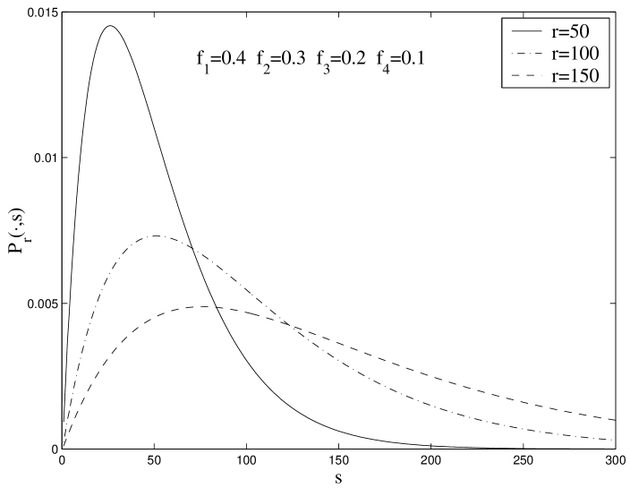
Figure 1: Numerical evaluation of $P_{r}(\cdot\,,s)$

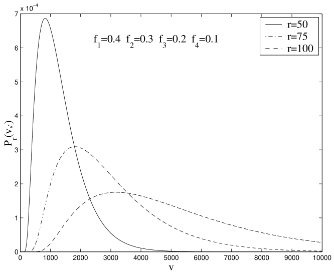
Figure 2: Numerical evaluation of $P_{r}(v,\cdot)$

IV.2 Expectation values and scaling

The expectation values for the volume and surface area, defined as

$${\mathrm{E}\!\left(s(x,r)\right)}=\sum_{s}sP_{r}(\cdot\,,s)=\left.\frac{\partial}{\partial\mu}G_{r}(1,\mu)\right|_{\mu=1}$$

$${\mathrm{E}\!\left(v(x,r)\right)}=\sum_{v}vP_{r}(v,\cdot)=\left.\frac{\partial}{\partial\lambda}G_{r}(\lambda,1)\right|_{\lambda=1}$$

can be explicitly calculated from the recursion rules; in fact for the first shell one simply gets

$${\mathrm{E}\!\left(s(x,1)\right)}=\langle z\rangle=2$$

$${\mathrm{E}\!\left(v(x,1)\right)}=3$$

while for larger values of $r$ the recurrence relations are easily found to read

$${\mathrm{E}\!\left(s(x,r+1)\right)}={\mathrm{E}\!\left(s(x,r)\right)}+2\alpha$$

and, quite obviously

$${\mathrm{E}\!\left(v(x,r+1)\right)}={\mathrm{E}\!\left(v(x,r)\right)}+{\mathrm{E}\!\left(s(x,r)\right)}+2\alpha$$

where

$$2\alpha=g^{\prime\prime}(1)=\langle z^{2}\rangle-4=\langle z^{2}\rangle-\langle z\rangle^{2}=(\Delta z)^{2}$$

Thus we obtain

$${\mathrm{E}\!\left(s(x,r)\right)}=2+2\alpha(r-1)\;,\quad{\mathrm{E}\!\left(v(x,r)\right)}=1+2r+\alpha(r-1)r$$ (18)

By further differentiating equation (12), one finds recursion rules for the expectation values of higher powers of $s(x,r)$ and $v(x,r)$ as well as of product of them (the moments of $P_{r}(v,s)$). By differentiating the logarithm of (12) one gets the centered, or connected moments. For instance, the general form of the connected surface moments is found to be

$${\mathrm{E_{c}}\!\left([s(x,r)]^{k}\right)}=c_{k}\alpha^{k}r^{k}+O(r^{k-1})$$ (19)

with $c_{k}$ constants; this fact suggests the scaling hypothesis that in the limit $r\to\infty$ of the shell probability must be a function only of the ratio $s/(\alpha r)$ (this is confirmed by the numerical determination in figure 1, after proper rescalings)

$$\alpha rP_{r}(\cdot\,,s)\ \overset{r\to\infty}{\sim}\phi\Big{(}\frac{s}{\alpha r}\Big{)}$$

where the factor $\alpha r$ on the left comes from the integration measure in the normalization:

$$1=\sum_{s=1}^{\infty}\frac{1}{\alpha r}\Big{(}\alpha rP_{r}(\cdot\,,s)\Big{)}\ \overset{r\to\infty}{\sim}\int_{0}^{\infty}d\tau\,\phi(\tau)$$ (20)

By the same token we see that the functions

$$F_{r}(u)=G_{r}\big{(}1,\exp(-\tfrac{u}{\alpha r})\big{)}=\sum_{s=1}^{\infty}\frac{1}{\alpha r}\Big{(}\alpha rP_{r}(\cdot\,,s)\Big{)}\exp(-\tfrac{us}{\alpha r})$$

should converge as $r\to\infty$ to the (continuous) Laplace transform $F(u)$ of the the scaling function $\phi(\tau)$

$$F_{r}(u)\ \overset{r\to\infty}{\sim}\int_{0}^{\infty}d\tau\,\phi(\tau)\,e^{-\tau u}\equiv F(u)$$

To calculate $F(u)$ we start from equation (15) and notice that the property (13) and the recursion $g_{r+1}(\mu)=g(g_{r}(\mu))$ imply $g_{r}(1)=g^{\prime}_{r}(1)=1$ for all $r$. This entails the scaling law

$$g_{r}\big{(}\!\exp(-\tfrac{u}{\alpha r})\big{)}=1+\frac{A(u)}{\alpha r}+o\bigg{(}\frac{1}{r}\bigg{)}$$

with $A(0)=0$ and $A^{\prime}(0)=-1$. Therefore

$$F_{r}(u)=-\alpha\,rg_{r}\big{(}\!\exp(-\tfrac{u}{\alpha r})\big{)}\frac{\partial}{\partial u}g_{r-1}\big{(}\!\exp(-\tfrac{u}{\alpha r})\big{)}\simeq-A^{\prime}(u)+o(1)$$ (21)

yielding the identification $F(u)=-A^{\prime}(u)$. Then the recursion rule for $g_{r}(\mu)$ to leading non–trivial order becomes the differential equation for $A(u)$

$$uA^{\prime}=A(1+A)$$

with the solution

$$A(u)=\frac{-u}{1+u}$$

Hence

$$F(u)=\frac{1}{\left(1+u\right)^{2}}$$ (22)

with the inverse Laplace transform

$$\phi(\tau)=\tau\,e^{-\tau}$$

so that the surface probability reads for large $r$

$$P_{r}(\cdot\,,s)\sim\frac{s}{\alpha^{2}r^{2}}\,e^{-s/(\alpha r)}$$ (23)

We may repeat this approach for the volume probabilities as well, by assuming a scaling form in the variable $v/(\alpha r^{2})$ (this would be obvious from the surface scaling for an homogeneous structure and is confirmed by the first connected moments and by the numerical data of figure 2). Thus we set (notice that $g(1)=1$ implies $h_{r}(1)=1$, see equation (17))

$$h_{r}\big{(}\!\exp(-\tfrac{\xi}{\alpha r^{2}})\big{)}=1+\frac{B(\xi)}{\alpha r}+o\bigg{(}\frac{1}{r}\bigg{)}$$

Substituting this expression in equation (17) we obtain to leading non–trivial order

$$2\xi B^{\prime}=B(1+B)-\xi$$

whose solution, taking care of the condition $B^{\prime}(0)=-1$ that comes from $h^{\prime}_{r}(1)=r$, reads

$$B(\xi)=-\sqrt{\xi}\tanh(\sqrt{\xi})$$

Now we set

$$G_{r}\big{(}\exp(-\tfrac{\xi}{\alpha r^{2}}),1\big{)}=H(\xi)+o(1)$$

so that

$$\frac{G_{r+1}\big{(}\exp(-\tfrac{\xi}{\alpha r^{2}}),1\big{)}}{G_{r}\big{(}\exp(-\tfrac{\xi}{\alpha r^{2}}),1\big{)}}\simeq 1+\frac{2\xi}{r}\frac{H^{\prime}(\xi)}{H(\xi)}+o\bigg{(}\frac{1}{r}\bigg{)}$$

and since for $\lambda=\exp(-\tfrac{\xi}{\alpha r^{2}})$

$$\lambda\,g^{\prime}(\lambda h_{r}(\lambda))\,\frac{h_{r+1}(\lambda)}{h_{r}(\lambda)}\simeq 1+\frac{2}{r}B(\xi)+o\bigg{(}\frac{1}{r}\bigg{)}$$

substituting these expressions in equation (16) we obtain the equation for $H(\xi)$

$$\xi H^{\prime}(\xi)=B(\xi)H(\xi)$$

and finally

$$H(\xi)=\frac{1}{(\cosh\sqrt{\xi})^{2}}$$ (24)

due to the normalization condition $H(0)=1$. The inverse Laplace transform of $H(\xi)$ is just the scaling form of the volume probabilities

$$\alpha r^{2}P_{r}(v,\cdot)\ \overset{r\to\infty}{\simeq}\Phi\Big{(}\frac{v}{\alpha r^{2}}\Big{)}$$

and may be written as (see Appendix A for details)

$$\Phi(\tau)=m^{1/4}\left(\frac{2K(m)}{\pi}\right)^{1/2}\left(\frac{2}{\pi}K(1-m)E(m)-1\right)$$ (25)

where

$$\tau=\frac{K(1-m)}{\pi K(m)}$$

and $K(m)$, $E(m)$ are the two complete elliptic integrals

$$K(m)=\int_{0}^{\pi/2}\frac{d\theta}{\sqrt{1-m\sin^{2}\!\theta}}\;,\quad E(m)=\int_{0}^{\pi/2}d\theta\sqrt{1-m\sin^{2}\!\theta}$$

The large $\tau$ behavior of $\Phi(\tau)$ follows in the limit $m\to 0$,

$$m\simeq 16\,e^{-\pi^{2}\tau}$$

and reads

$$\Phi(\tau)\simeq(\pi^{2}\tau-2)\,e^{-\pi^{2}\tau/4}\;,\quad\tau\to\infty$$

The behavior for small $\tau$ is related to that for $m\to 1$,

$$1-m\simeq 16\,e^{-1/\tau}$$

so that

$$\Phi(\tau)\simeq\frac{4}{\sqrt{\pi}}\,\tau^{-3/2}\,e^{-1/\tau}\;,\quad\tau\to 0$$

Therefore the volume probability distribution has the large $r$ asymptotic behavior

$$P_{r}(v,\cdot)\simeq\begin{cases}\dfrac{4\,\alpha^{1/2}r}{\pi^{1/2}v^{3/2}}\,e^{-\alpha r^{2}/v}&\text{for }v\ll r^{2}\vspace{3mm}\\ \vspace{2mm}\dfrac{\pi^{2}v}{\alpha^{2}r^{4}}\,e^{-\pi^{2}v/(4\alpha r^{2})}&\text{for }v\gg r^{2}\end{cases}$$ (26)

IV.3 Local and average connectivity dimensions

The results of the previous section concern the probability distributions for the growth around $x$ in the statistical ensemble of infinite trees rooted at $x$. To relate these results to graph averages over a single “generic” realization of such a tree, we consider the following observables

$${\bar{P}}_{r}(v)=\frac{1}{v(x,R-r)}\sum_{y\in B(x,R-r)}\delta(v(y,r)-v)$$

that are the fractions of nodes $y$ for which the ball of radius $r$ has volume $v$ in a specific realization of a tree rooted at $x$ (restricted to radius $R$). In the limit of $R\to\infty$ the natural ergodic, or better autoaveraging hypothesis is that ${\bar{P}}_{r}(v)$ deviates from its expectation value ${\mathrm{E}\!\left({\bar{P}}_{r}(v)\right)}$ only on a subset of measure zero of the statistical ensemble and that ${\mathrm{E}\!\left({\bar{P}}_{r}(v)\right)}$ coincides with $P_{r}(v,\cdot)$, the previously calculated probability

$$\lim_{R\to\infty}\Delta{\bar{P}}_{r}(v)=0\;,\quad\lim_{R\to\infty}{\mathrm{E}\!\left({\bar{P}}_{r}(v)\right)}=P_{r}(v,\cdot)$$ (27)

As a matter of fact, the results reported in section III.2 are enough to conclude that this autoaveraging is not simply an hypothesis: let us fix the size $r$ of balls $B(y,r)$ centered on arbitrary nodes and consider the local finite branching process rooted on $y$ that reconstructs $B(y,r)$; if $y$ dists more than $r$ from from the spine this process is distributed exactly like that rooted on $x$; if two such processes are rooted on nodes well separated, they are independent; the number of nodes closer than $r$ to the spine scales with $R$, the size of the main process, as compare to the volume $v(x,R-r)$ that scales as $R^{2}$; from the (weak) law of large numbers we then expect (27) to hold. We have performed several numerical checks that confirm this expectation with high accuracy (see section IV.4)

We conclude therefore, by looking at the main results (26), that the local connectivity (or intrinsic Hausdorff) dimension $d_{\rm c}$ of section II.1 exists and that $d_{\rm c}=2$ with probability one. Moreover, ${\bar{d}}_{\rm c}=d_{\rm c}$ because, thanks to (27), we can substitute the expectation value ${\mathrm{E}\!\left(v(x,r)\right)}$ in (18) with the graph average $\langle v(r)\rangle$ for a single random tree.

IV.4 Numerical checks

We have performed several numerical checks of the autoaveraging property discussed above; for example figure 3 compares the distribution of $\tau=v(y,r)/(\alpha r^{2})$ for $3\cdot 10^{5}$ nodes $y$ on a graph of $10^{7}$ nodes with $r=500$, with the calculated limit distribution $\Phi(\tau)$.

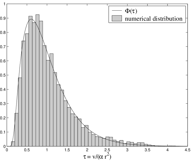
Figure 3: Comparison between the distribution of $v(y,r)/r^{2}$ ($r=500$) in a graph and $\Phi(\tau)$

Another check can be done in the case of $v_{z}(x,r)$, since its average over different realizations of the graph–generating algorithm can easily be calculated and compared with the numerically obtained average over different nodes on a single graph. The spinal decomposition and the considerations in the previous section allow us to write

$$\begin{split}{\mathrm{E}\!\left(v_{z}(x,r)\right)}&=\tilde{f}_{z}r+({\mathrm{E}\!\left(v(x,r)\right)}-r)f_{z}\\ &=f_{z}\big{(}1+(z-\alpha)r+\alpha r^{2}\big{)}\end{split}$$

with the use of equation (18). In figure 4 we have plotted ${\mathrm{E}\!\left(v_{z}(x,r)\right)}/(f_{z}{\mathrm{E}\!\left(v(x,r)\right)})$ compared with the corresponding average over $3\cdot 10^{4}$ nodes of a single random tree with $10^{7}$ nodes.

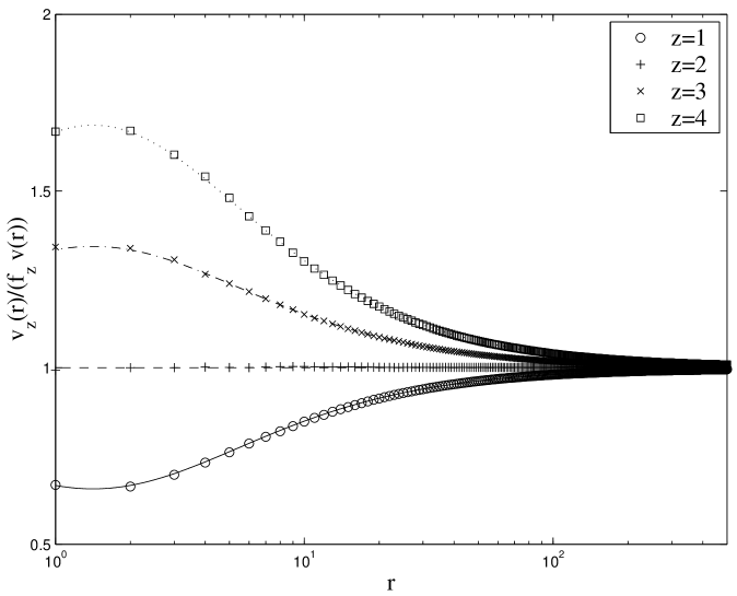
Figure 4: Comparison between numerical averages over $3\cdot 10^{4}$ nodes of a single tree with $10^{7}$ and expectation values. Error bars are smaller than the size of symbols

Appendix A Inverse Laplace transform of $H(\xi)$

The inverse Laplace transform of $H(\xi)$, $\Phi(\tau)$ is defined to be

$$\Phi(\tau)=\frac{1}{2\pi i}\int_{\gamma-i\,\infty}^{\gamma+i\,\infty}d\xi H(\xi)\exp(\tau\xi)$$

where $\gamma$ is an arbitrary positive constant chosen so that the contour of integration lies to the right of all singularities in $H(\xi)$. In this case $H(\xi)$ is given by equation (24)

$$H(\xi)=\frac{1}{(\cosh\sqrt{\xi})^{2}}$$

and its singularities in the complex plane of the variable $\xi$ are located in

$$\xi_{n}=-\pi^{2}\Big{(}n+\frac{1}{2}\Big{)}^{2}\qquad n=0,1,2,\ldots$$

and the residue of $H(\xi)\exp(\tau\xi)$ in $\xi_{n}$ reads

$$\text{Res}[H(\xi)\exp(\tau\xi),\xi_{n}]=\left(\pi^{2}(2n+1)^{2}\tau-2\right)e^{-\pi^{2}(n+1/2)^{2}\tau}$$

Now using the residue theorem

$$\begin{split}\Phi(\tau)&=\sum_{n=0}^{\infty}\text{Res}[H(\xi)\exp(\tau\xi),\xi_{n}]\\ &=\sum_{n=0}^{\infty}\left(\pi^{2}(2n+1)^{2}\tau-2\right)e^{-\pi^{2}(n+1/2)^{2}\tau}\\ &=(-2\tau\frac{\partial}{\partial\tau}-1)\ \theta_{2}(0,e^{-\pi^{2}\tau})\end{split}$$ (28)

where $\theta_{2}(u,q)$ is the second elliptic theta function with argument $u$ and nome $q$; for $u=0$ it can be expressed in terms of the complete elliptic integral $K(m)$

$$\theta_{2}(0,e^{-\pi^{2}\tau})=\left(\frac{2m^{1/2}K(m)}{\pi}\right)^{1/2}$$

with $m$ obtained by inverting

$$\tau=\frac{K(1-m)}{\pi K(m)}$$

Using the identities

$$\frac{\partial}{\partial m}K(m)=\frac{E(m)-(1-m)K(m)}{2m(1-m)}$$

and

$$K(m)E(1-m)+K(1-m)E(m)-K(m)K(1-m)=\frac{\pi}{2}$$

we obtain

$$-2\tau\frac{\partial}{\partial\tau}=\frac{8}{\pi}m(1-m)K(m)K(1-m)\frac{\partial}{\partial m}$$

and finally equation (25)

$$\Phi(\tau)=m^{1/4}\left(\frac{2K(m)}{\pi}\right)^{1/2}\left(\frac{2}{\pi}K(1-m)E(m)-1\right)$$

Now the asymptotic behavior for $\tau\to\infty$ and $\tau\to 0$ can be found using the expansions

$$K(m)\simeq \frac{\pi}{2}\big{(}1+\frac{m}{4}\big{)} \text{for }m\to 0$$

$$E(m)\simeq \frac{\pi}{2}\big{(}1-\frac{m}{4}\big{)} \text{for }m\to 0$$

$$K(m)\simeq \log 4-\frac{1}{2}\log(1-m)+\frac{1}{4}(1-m)\left(\log 4-\frac{1}{2}\log(1-m)-1\right) \text{for }m\to 1$$

$$E(m)\simeq 1+\frac{1}{4}(1-m)\left(2\log 4-\log(1-m)-1\right) \text{for }m\to 1$$

For $m\to 0$ one can obtain

$$\tau\simeq\frac{4\log 2-\log m}{\pi^{2}}$$

$$m\simeq 16\,e^{-\pi^{2}\tau}$$

so that the asymptotic behavior $\Phi(\tau)$ for $\tau\to+\infty$

$$\begin{split}\Phi(\tau)&\simeq m^{1/4}\big{(}\log 4-\frac{1}{2}\log m-1\big{)}\\ &\simeq(\pi^{2}\tau-2)\,e^{-\pi^{2}\tau/4}\end{split}$$

tar that is simply the first term in the series equation (28).

For $m\to 1$ the variable change reads

$$\tau\simeq\frac{1}{4\log 2-\log(1-m)}$$

$$1-m\simeq 16\,e^{-1/\tau}$$

so that for $\tau\to 0$

$$\begin{split}\Phi(\tau)&\simeq\bigg{(}\frac{1-m}{4}\bigg{)}\big{(}4\log 2-\log(1-m)\big{)}^{3/2}\\ &\simeq\frac{4}{\sqrt{\pi}}\,\tau^{-3/2}\,e^{-1/\tau}\end{split}$$

List of figures

1. Numerical evaluation of $P_{r}(\cdot\,,s)$

2. Numerical evaluation of $P_{r}(v,\cdot)$

3. Comparison between the distribution of $v(y,r)/r^{2}$ ($r=500$) in a graph and $\Phi(\tau)$

4. Comparison between numerical averages over $3\cdot 10^{4}$ nodes of a single tree with $10^{7}$ and expectation values.

References

- (1) D. Stauffer and A. Aharony, Introduction to percolation theory,Taylor & Francis, London (1994)
- (2) T. Jonsson, J.F. Wheater, Nucl. Phys. B 515 (1998) 549
- (3) R. Burioni, D. Cassi, Phys. Rev. E 51, 2865 (1995)
- (4) M.Suzuki, Progr, Theor. Phys. 69, 65 (1983)
- (5) G.H. Weiss S. Havlin,Physica A 134, 474 (1986)
- (6) R. Burioni, D. Cassi, A. Vezzani, Eur. Phys. J. B 15, 665 (2000)
- (7) K.B. Athreya, P.E. Ney, Branching Processes, Springer–Verlag, New York (1972)
- (8) H. Kesten, Ann. Inst. H. Poincaré Probab. Statist. 22, 425 (1987)
- (9) D. Aldous, J. Pitman, Ann. Inst. H. Poincaré 34, 637 (1998)